Abstract
A typical retailer carries 10,000 stock-keeping units (SKUs). However, these numbers may exceed hundreds of millions for giants such as Walmart and Amazon. Besides the volume, SKU data can also be high-dimensional, which means that SKUs can be segmented on the basis of various attributes. Given the data volumes and the multitude of potentially important dimensions to consider, it becomes computationally impossible to individually manage each SKU. Even though the application of clustering for SKU segmentation is common, previous studies do not address the problem of parametrization and model finetuning, which may be extremely tedious and time-consuming in real-world applications. Our work closes the research gap by proposing a solution that leverages automated machine learning for the automated cluster analysis of SKUs. The proposed framework for automated SKU segmentation incorporates minibatch K-means clustering, principal component analysis, and grid search for parameter tuning. It operates on top of the Apache Parquet file format, an efficient, structured, compressed, column-oriented, and big-data-friendly format. The proposed solution was tested on the basis of a real-world dataset that contained data at the pallet level.
1. Introduction
Supply chains encompass manufacturing procurement, material handling, transportation, and distribution [1]. Demand propagates upstream as the information flow and supply responses in the form of commodity flow. However, supply cannot immediately match the demand due to various physical limitations involved in this process. For example, factories can produce only a certain number of items, trucks cannot exceed speed limits, and the capacity and number of container ships are constrained. The lead times might also be several weeks or even months in global supply chains. In this regard, inventory management is essential, since the inventory plays the role of a buffer against uncertainty and ensures business continuity across supply chains [2].
The importance of managing inventory is also illustrated by the US Department of Commerce, which regularly keeps track of inventory value held in different parts of the supply chain. In April 2022, USD 2.27 trillion were held in inventory across all types of business [3]. The retail industry alone accounted for USD 662 billion, approximately 17% of which was held by e-commerce [4]. As Figure 1 shows, these values recovered from the pandemic shocks and are on the rise.
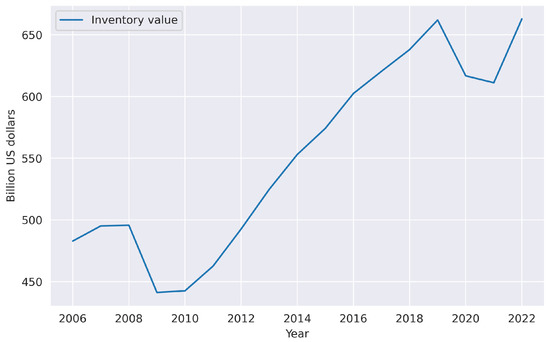
Figure 1.
Value of inventories held for sale at the retail level. The figure was produced on the basis of data reported by the U.S. Census Bureau [3].
Humanity has engaged in inventory management, at least in some primitive form, since it started gathering and stockpiling the planet’s resources. However, the rigorous approach of prioritizing items for management attention can be dated back to Joseph Moses Juran [5]. Since a typical inventory system could contain an immense number of items with unique characteristics such as price, demand, and physical properties, analyzing them individually would outstrip anyone’s managerial effort and attention. That is why retailers frequently use stock-keeping-unit (SKU) segmentation to guide themselves in planning, buying, and allocating products [6]. The common purposes for SKU segmentation include:
- Selecting an appropriate inventory control policy [7,8].
- Understanding the demand patterns [9].
- Optimal allocation under the limited storage capacity [10].
- Selecting an appropriate supply-chain strategy [9].
- Evaluating the environmental impacts of inventory throughout its life cycle [11].
Every customer sees SKUs on a daily basis as barcodes in the grocery stores or items on the e-commerce platforms. A typical retailer carries 10,000 SKUs [6]. For giants such as Walmart, the number exceeds 75 million [12]. However, the e-commerce industry typically operates with an even more extensive catalog of items. A genuinely gargantuan case is the Amazon marketplace, acting as the home for more than 350 million SKUs [13]. Considering the extension of the supply chain directly into inhand devices through the adoption of digital technologies, and consumers’ impatience, the future scale of the e-commerce industry can be expected to skyrocket.
Besides the volume, SKU data can also be distinguished by the high dimensionality, which means that SKUs can be segmented on the basis of various attributes. The most traditional way is the ABC classification method, which segments the SKUs on the basis of sales volume. The underlying theory of this segmentation method is the 20–80 Pareto principle. The principle suggests that 20% of SKUs generate approximately 80% of total revenue. Therefore this 20% should constitute the category that deserves the most attention from management. ABC segmentation utilizes only one dimension to segment the SKUs that, on the first hand, facilitates implementation [14]. However, on the other hand, SKUs within the segment can have substantially different characteristics. For example, two SKUs may have similar contributions to the revenue, but one may have a high unit price but low demand, and the other may have a low unit value but high demand. Indeed, it would be wrong to manage these SKUs under the same strategy. The physical properties of the SKU are another example. ABC segmentation does not consider perishability, which is essential for grocery retail. The weight and height of the loaded pallet can be crucial if the business operates under the constrained storage space, which is the case for retail chains in dense urban areas [10].
Given the data volumes and the multitude of potentially important dimensions to consider, it becomes computationally impossible to individually manage each SKU. In this regard, the prominent question arises: “How to aggregate SKUs so that the resulting management policies are close enough to the case where each SKU is considered individually?” Our paper aims to answer this long-standing question by taking advantage of state-of-the-art big-data technologies and automated machine-learning (AutoML) approaches [15].
The remainder of this paper is organized as follows. Section 2 presents the related work and highlights the research gap. Section 3 introduces the methodology at a high level and provides the rationale behind the choice of the individual components. Section 4 demonstrates how the proposed framework functions on the basis of a real-world dataset. Section 5 highlights the potential advantages of the proposed framework, and discusses several use cases along with managerial implications. Lastly, Section 6 summarizes the paper and suggests promising directions for future research.
2. Related Work and Novelty
Considering the size and dimensionality of SKU data, and the market pressure on businesses to make critical decisions quickly, it is frequently not computationally feasible to treat every item individually. An alternative would be to define groups while taking into account all product features that notably influence the operational, tactical, or strategic problem of interest. These features can vary depending on the problem of interest, and go beyond the revenue and demand attributes used in classical ABC analysis. Clustering in particular and unsupervised machine learning in general are the most natural approaches to creating groups of SKUs that share similar characteristics [16].
Early attempts to group SKUs using cluster analysis go back to Ernst and Cohen, who proposed the operations related groups method to consider a full range of operationally significant item attributes. The method is similar to factor analysis and allows for considering a full range of operationally significant item attributes. The method was initially designed to assist an automobile manufacturer with developing inventory control policies [7]. Shortly after that, Srinivasan and Moon introduced a hierarchical-clustering-based methodology to facilitate inventory control policies in supply chains [17]. Hierarchical clustering still remains a popular technique. For instance, in a recent study, the authors proposed a hierarchical segmentation for spare-part inventory management [18]. Even though such an approach is simple to implement and interpret, hierarchical clustering has several fundamental shortcomings. First, the method does not scale well because of the computational complexity compared to more efficient algorithms, such as K-means. Second, hierarchical clustering is biased towards large clusters and tends to break them. Third, in hierarchical clustering, the order of the data impacts the final results. Lastly, the method is sensitive to noise and outliers [19].
Currently, K-means is the most popular clustering technique [20]. The algorithm is appealing in many aspects, including computational and memory efficiency, and interpretability in low-dimensional cases. The notable applications to SKU segmentation include Canneta et al., who combined K-means with self-organizing maps to cluster products across multiple dimensions [21]. Wu et al. applied K-means along with correlation analysis to identify primary indicators to predict demand patterns [22]. Egas and Masel used K-means clustering to reduce the time required to derive the inventory-control parameters in a large-scale inventory system. The proposed method outperformed a demand-based assignment strategy [23]. Ozturk et al. used K-means to obtain SKU clusters. Then, an artificial neural network was applied to forecast demand for each individual cluster [24].
It is also essential to highlight the applications of fuzzy C-means to SKU segmentation. Fuzzy C-means is a form of clustering in which a cluster is represented by a fuzzy set. Therefore, each data point can belong to more than one cluster. Notable applications include multicriteria ABC analysis using fuzzy C-means clustering [25]. A recent study by Kucukdeniz and Sonmez proposed the integrated order-picking strategy based on SKU segmentation through fuzzy C-means. In this study, fuzzy clustering was applied to consider the order frequency of SKUs and their weights while designing the warehouse layout [26]. Fuzzy C-means is an interesting alternative to K-means. However, the fact that each SKU can belong to more than one cluster is a disadvantage in the business context. Since businesses must quickly and confidently make critical yes/no decisions, the fuzziness of SKU segments does not provide any helpful flexibility for decision making at scale, and introduces unnecessary layers of complexity. Additionally, the fuzzy C-means method has the same drawbacks as those of classical K-means. The drawbacks include the a priori specification of the number of clusters, poor performance on datasets that contain clusters with unequal sizes or densities, and sensitivity to noise and outliers [27].
In order to overcome the aforementioned shortcomings, preprocessing and dimensionality reduction techniques like PCA are applied to SKU data prior to clustering. For example, the authors conducted a study on the application of a constrained clustering method reinforced with principal component analysis. According to the research, the proposed method can provide significant compactness among item clusters [28]. Another study took advantage of PCA and K-means to segment SKUs for recommendation purposes [29]. In recent work, Bandyopadhyay et al. used PCA prior to K-means to achieve the effective segmentation of both customers and SKUs in the context of the fashion e-commerce industry [29].
Table 1 lists the aforementioned clustering-based approaches to SKU segmentation and groups them in accordance with the utilized method. Even though the combination of K-means and PCA helps in overcoming some critical problems such as sensitivity to noise and multicollinearity, it does not address the parametrization problem, namely, the a priori specification of the number of clusters. Moreover, parametrization becomes even more sophisticated because the potential user must choose the number of principal components for PCA. The problem of parametrization and model finetuning can be extremely tedious and time-consuming in real-world applications. That is why our work attempts to close the research gap by proposing a framework that leverages AutoML for the automated cluster analysis of SKUs.

Table 1.
Approaches to SKU segmentation.
3. Materials and Methods
Summarizing the related work, we represent the data pipeline in the following flexible form: data storage and retrieval, preprocessing and standardization, dimensionality reduction (PCA), and clustering (K-means). Figure 2 shows an example of such a pipeline visualized using Orange, a Pythonic data mining toolbox [30]. The pipeline is flexible and capable of segmenting SKUs in the unsupervised learning setting, which is crucial since the class values corresponding to an a priori partition of the SKUs are not known [31].
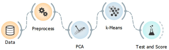
Figure 2.
Typical data pipeline for SKU segmentation.
The popularity of K-means can be justified by the fact that more sophisticated clustering techniques such as mean shift [32] and density-based spatial clustering of applications with noise (DBSCAN) [33] do not allow for one to explicitly set the number of clusters (k in K-means). The finetuning of these algorithms is nontrivially performed by selecting “window size” for mean shift and “density reachability” for DBSCAN. Additionally, the algorithms do not perform well if SKU data contain convex clusters with significant differences in densities.
The incorporation of PCA, on the other hand, allows for one to improve the clustering results for two main reasons. First, SKU features can share mutual information and correlate with each other. Second, it is natural for SKU data to contain some portion of noise due to the measurement or recording error. On that basis, PCA could be helpful as a tool in decorrelation and noise reduction [8].
3.1. Data Storage
The underlying data layout, including file format and schema, is an essential aspect in obtaining high computational performance and storage efficiency. The proposed framework for automated cluster analysis works on top of the Apache Parquet file format. Apache Parquet is an efficient, structured, compressed, binary file format that stores data in a column-oriented way instead of by row [34]. As a result, the values in each column are physically stored in contiguous memory locations, which provides the following crucial benefits:
- Data are stored by column instead of by row. Columnwise compression is space-efficient because the specific compression techniques to a data type can be applied at the column level.
- Query processing is more efficient as the columns are stored together. This is because the query engine can fetch only specific column values, skipping the columns that are not needed for a particular query.
- Different encoding techniques can be applied to different columns, drastically reducing storage requirements without sacrificing query performance [35].
As a result, Parquet provides convenient and space-efficient data compression and encoding scheme with enhanced performance to operate with complex multidimensional and multitype data.
3.2. Feature Scaling
Feature scaling, also known as data normalization, is an essential step in data preprocessing. Machine-learning techniques such as K-means use distances between data points to determine their similarity that render them especially sensitive to feature scaling. The primary role of feature scaling in ML pipelines is to standardize the independent variables, so they are in a fixed range. If feature scaling is not performed, K-means weigh variables with greater absolute values higher, severely undermining the clustering outcome [36].
The proposed framework for automated cluster analysis uses min–max scaling, the most straightforward method that scales features, so they are in the range of [0, 1]. The min–max scaling is performed according to the following formula:
where x is an original value and is the normalized one.
3.3. Clustering
K-means is the most straightforward clustering method and, as the related work section revealed, is widely adopted for SKU segmentation purposes. K-means splits n observations (SKUs in the context of this study) into k clusters. Formally, given a set of SKUs , where each SKU is a feature vector, K-means segments x into k sets minimizing the within-cluster sum of squares, also known as inertia .
The proposed framework for automated cluster analysis incorporates minibatch K-means, a variant of K-means clustering that operates with so-called minibatches to decrease computational time while still attempting to minimize inertia. Minibatches refer to the randomly and iteratively sampled subsets of the input data. This approach significantly reduces the computational budget required to converge to a nearly optimal solution [37]. Algorithm 1 demonstrates the key principle behind minibatch K-means. The algorithm iterates between two crucial steps. In the first step, observations are sampled randomly to form a minibatch. Then, the minibatch is assigned to the nearest centroid that updates in the second step. In contrast to the standard K-means algorithm, the centroid updates are conducted per sample. These two steps are performed until convergence, or a predetermined stoppage criterion is met.
| Algorithm 1 Minibatch K-means [37]. |
|
3.4. Dimensionality Reduction
Observations originated from natural phenomena or industrial processes frequently contain a large number of variables. A multitude of SKU features that can potentially impact operational and strategic decisions is a notable example. Therefore, the data analysis pipelines can benefit from dimensionality reduction in one form or another. In general, dimensionality reduction can be defined as the transformation of data into a low-dimensional representation, so that the obtained representation retains meaningful properties and patterns of the original data [38]. Principal component analysis (PCA) is the most widely adopted and theoretically grounded approach to dimensionality reduction. The proposed framework for automated cluster analysis incorporates PCA in order to decompose a multidimensional dataset of SKUs into a set of orthogonal components, such that the set of the obtained orthogonal components has a lower dimension, but is still capable of explaining a maximal amount of variance [39].
Computation for PCA starts with considering the dataset of n SKUs with m features. The SKU dataset can be represented as the following matrix:
where is a ith row vector of length m. Thus, is a matrix whose columns represent features of a given SKU.
The sample means and standard deviations can be defined with respect to the columns and . After that, the matrix can be standardized as follows:
where stands for a matrix.
Covariance matrix can be defined as . So, we can finally perform a standard diagonalization as follows:
where eigenvalues are arranged in descending order: . Transformation matrix is the orthogonal eigenvector matrix. The rows are the principal components of , and the value of represents the variance associated with the ith principal component [39].
3.5. Validation
Since the ground truth is not known, clustering results must be validated on the basis of an internal evaluation metric. Generally, inertia gives some notion of how internally coherent clusters are. However, the metric suffers from several disadvantages. For example, it assumes that clusters are convex and isotropic, which is not always the case with SKUs. Additionally, inertia is not a normalized metric, and Euclidean distances tend to inflate in high-dimensional spaces. Fortunately, the latest can be partially alleviated by PCA [40].
Unsupervised learning in general and clustering in particular approach the problem, which is biobjective by nature. On the one hand, data instances must be partitioned, such that points in the same cluster are similar to each other (this property is also known as cohesion). On the other hand, clusters themselves must be different from each other (a property known as separation). The silhouette coefficient is explicitly designed to evaluate the clustering results taking into account both cohesion and separation. The Silhouette coefficient is calculated for each sample and is composed of two components (a and b).
where a is the mean distance between a sample and all other points within the same cluster (measure of cohesion). b is the mean distance between a sample and all other points in the next nearest cluster (measure of separation) [41].
3.6. Parameter Optimization
Parameter optimization is a common problem in SKU segmentation, and a distinct issue from the process of dimensionality reduction and solving the clustering problem itself. Parameter optimization in the context of the unsupervised learning-based SKU segmentation is the process of determining the optimal number of clusters in a data set (k in K-means) and the optimal number of principal components (p in PCA) [42]. If appropriate values of k and p are not apparent from prior knowledge of the SKU properties, they must be defined somehow. That is where the elements of AutoML come into play. Grid search or a parameter sweep is the traditional way of performing parameter optimization [43]. The method performs an exhaustive search through a specified set of parameter space guided by the Silhouette score.
The proposed framework for automated cluster analysis is built on top of the pipeline that has two hyperparameters to be finetuned. Namely, the number of clusters and the number of principal components . Two sets of hyperparameters K and P can be represented as a set of ordered pairs , also known as Cartesian product . Grid search then trains the pipeline with each pair and outputs the settings that achieved the highest Silhouette score.
Grid search suffers from the curse of dimensionality, but since the parameter settings that it evaluates are independent of each other, the parallelization process is straightforward, allowing for one to leverage the specialized hardware and cloud solutions [44].
Implementation
The proposed framework for automated cluster analysis was implemented entirely in Python. The reading of the data from the Apache Parquet file format and all the manipulations with the data structures were performed using Pandas [45], which was optimized for performance, with critical code paths written in such low-level programming languages as Cython and C [46].
The unsupervised learning components, including K-means and PCA, were implemented using scikit-learn, an open-source ML library for Python [47]. The scikit-learn implementation of K-means uses multiple processor cores benefiting from multiplatform shared-memory multiprocessing execution in Cython. Additionally, data are processed in chunks of 256 samples in parallel, which results in a low memory footprint [48]. The scikit-learn implementation of PCA was based on [49]. The data visualization was performed using Seaborn, a Python data visualization library [50].
4. Results
The proposed framework was tested on the basis of a real-world dataset that contains SKU data of perishable grocery products at the pallet level. The dataset was provided by a third-party logistics provider from the Baltic region and contained data at the pallet level. The study was conducted in a reproducible manner. The data availability section at the end of this manuscript contains the link to the GitHub repository with the source code and original dataset.
4.1. Dataset Description
The dataset included 1218 rows that corresponded to the individual SKUs and 4 columns corresponding to SKU attributes or features. The features included unit price (EUR), number of units per pallet, gross weight of the loaded pallet (kg), and Pallet height (m).
Table 2 provides descriptive statistics, including measures of central tendency, dispersion, and quartiles. Figure 3 sheds light on the shape of the feature’s distribution by presenting the box plots and kernel density estimation plots. The kernel density estimation plots are produced by applying kernel smoothing to estimate the probability density function of the empirical data. Such an illustration immediately provides critical insights into the data structure. Such features as “unit price”, “number of units”, and “gross weight” are heavy-tailed and multimodal (trimodal to be more specific).
Table 2.
Measures of central tendency, dispersion, and quartiles.
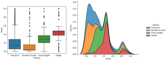
Figure 3.
Box plots and kernel density estimation plots of the SKU features.
It is also essential to check the presence of multicollinearity in the dataset. The Pearson correlation coefficient is the most straightforward approach to measuring the linear relationship between two features. The coefficient varies between −1 and +1, with correlations of −1 or +1 implying an exact linear relationship and 0 implying no correlation [51]. Table 3 contains Pearson’s correlation coefficient and the corresponding p-values. The p-values indicate the probability of a pair of uncorrelated features having a correlation coefficient to be at least as extreme as the one calculated on the basis of data [51].
Table 3.
Pearson correlation coefficient with corresponding p-values.
Even though K-means clustering is not severely affected by the presence of multicollinearity, correlation coefficients may provide a hint of whether PCA has the potential of improving clustering results. Besides that, the computation of correlation coefficients and plotting the features pairwise could reveal the data structure and provide valuable managerial insights. Figure A1 provides the bivariate view illustrating the relationship between two of the most correlated features, “gross weight” and “unit price”, and describing the strength of their relationship. Figure A2 illustrates the pairwise relationships in a dataset. The diagonal plots correspond to a univariate distribution plot demonstrating the marginal distribution of each feature.
4.2. Numerical Experiment
In order to test the proposed framework, the grid search was performed across the search space produced by the Cartesian product of and , where corresponded to the case where PCA was not applied. Figure 4 shows Silhouette scores of the pipeline with each pair of parameters.
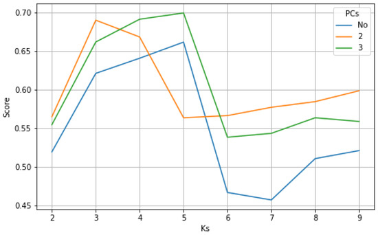
Figure 4.
Silhouette scores calculated across the Cartesian product.
The pipeline with three principal components and five clusters demonstrated the highest performance (Silhouette score of 0.699). Additionally, five clusters appeared to be optimal even when PCA had not been applied. However, such a pipeline performed notably worse (Silhouette score of 0.662). The pipeline with two principal components and three clusters could be considered as an alternative with the second best performance (Silhouette score of 0.690). Table A1 contains the Silhouette score values for every pair of pipeline parameters obtained through the grid-search procedure.
In a real-world setting, decision making could be driven not only by the performance metric, but also by a plethora of other factors and considerations. For example, even though the SKU segmentation with three principal components and five clusters yielded the highest Silhouette score, the priority may be given to the second best solution (two principal components and three clusters) because fewer clusters are easier to manage. This relatively simple case reveals an additional advantage of the proposed framework. Namely, it provides and ranks multiple solutions, but it is up to a manager to make a final decision considering other factors (potentially non-numerical) initially not taken into account by the algorithm. Figure A3 shows the pairwise view of the clustering results. The diagonal plots demonstrate the marginal distribution of each feature within each cluster. On the basis of visualizations, the potential end user could conclude that the produced SKU clusters are homogeneous to be treated under common inventory management or material handling policy.
5. Discussion
This chapter discusses our research contributions and the technological advantages of the proposed implementation. It also discusses several use cases and provides managerial implications.
5.1. Research Contributions
The idea of prioritizing items for management attention dates back to the 1950s [5], and the first attempt to cluster SKUs dates back to the 1990s [7]. As time progresses, new clustering techniques are applied to this longstanding problem. Nowadays, the most common techniques include hierarchical clustering, K-means, fuzzy C-means, and K-means combined with PCA.
Even though hierarchical clustering is simple to implement and interpret at the managerial level, it does not scale well because of the computational complexity. The algorithm is also biased towards large clusters and tends to break them even if it leads to suboptimal segmentation. The method is also sensitive to noise and outliers [19].
K-means is appealing in many aspects, including computational and memory efficiency, and interpretability in low-dimensional cases [20]. However, the method requires the number of clusters to be specified in advance. In business applications, the a priori specification of the number of clusters is a severe drawback because it requires an additional effort to parametrize and finetune the model. Additionally, K-means performs poorly on datasets that contain clusters with unequal sizes or densities, and is also sensitive to both noise and outliers [20].
Fuzzy C-means is an alternative to K-means that treats a cluster as a fuzzy set, allowing for SKUs to belong to more than one cluster. This approach may have theoretical importance. However, the fact that each SKU can belong to more than one cluster is a clear disadvantage in the business context. Since supply chains operate under pressure from both supply and demand, businesses have to make critical decisions quickly and confidently. Therefore, the fuzziness of SKU segments does not provide any helpful flexibility for decision making at scale, and introduces unnecessary layers of complexity to decision making [27].
In order to overcome the mentioned shortcomings, preprocessing and dimensionality reduction techniques such as PCA are applied to SKU data prior to clustering. The incorporation of PCA allows for one to improve the clustering results through decorrelation and noise reduction [38]. However, even though the combination of K-means and PCA helps to overcome some critical problems, it further worsens the parametrization and finetuning problem because the potential user must choose the number of principal components and the number of clusters. Our work closes this research gap by proposing to automate parametrization and finetuning. We propose an AutoML-based framework for SKU segmentation that leverages grid search along with the computationally efficient and parallelism-friendly implementations of clustering and dimensionality reduction algorithms. The following subsections shed light on the technological advantages of the proposed solution and managerial implications.
5.2. Technological Contributions
The proposed framework for automated cluster analysis can work with SKU features beyond that utilized by a classical ABC approach. The framework operates in an unsupervised learning setting, which is crucial since class values corresponding to an a priori partition of the SKUs are not known. The optimal number of clusters in a dataset and the optimal number of principal components are determined through the grid search in a fully automated fashion using the Silhouette score as a performance estimation metric.
In a real-world setting, decision making could be less straightforward and incorporate unquantifiable metrics. In this regard, the critical advantage of the framework is that the grid search examines every possible solution within the search space and ranks them in accordance with the Silhouette score. Therefore, the end user can select a solution that is aligned with some potentially unquantifiable managerial insights, but is not necessarily best according to the performance estimation criteria. Additionally, the framework is equipped with data-visualization capabilities, which give end users the ability to diagnose the segmentation validity, choose among alternative solutions, and effectively communicate results to the critical stakeholders.
The proposed framework is strongly associated with the so-called “no free lunch” theorem. According to the theorem, there cannot exist a superior algorithm to any competitive one across the domain of all possible problems [52]. In this regard, the question of whether the proposed framework is inferior or superior to the potential alternative is meaningless, since its performance would depend on the data generation mechanism and distribution of feature values. Nevertheless, the following properties should be highlighted as the indisputable practical advantages of the proposed approach:
- Automatism. Such labor-intensive and time-consuming steps as parameter optimization and finetuning are fully automated and do not require the participation of data scientists or other human experts.
- Parallelism. The proposed framework for automated cluster analysis incorporates minibatch K-means, a computationally cheap variant of K-means clustering. The implementation of minibatch K-means uses multiple processor cores benefiting from multiplatform shared-memory multiprocessing execution in Cython. Additionally, data are processed in chunks of 256 samples in parallel. The parallelization process for the grid search is straightforward as well, which allows for one to leverage the specialized hardware and cloud solutions.
- Big-data-friendliness. The proposed framework operates on top of the Apache Parquet file format, an efficient, structured, compressed, partition-friendly, and column-oriented data format. The reading of the data from the Apache Parquet file format and all the manipulations with the data structures were performed using Pandas, which was optimized for performance.
- Interpretability. Data-visualization capabilities allow for a potential user to diagnose the segmentation validity, spot outliers, gain critical insights regarding the data structure, and effectively communicate results to the critical stakeholders.
- Universality. The optimal number of clusters in a dataset and the optimal number of principal components are usually not apparent from prior knowledge of the SKU properties. Since the proposed framework performs an exhaustive search through a specified set of parameters, it may be applied to any SKU dataset with numeric features or even extended to similar domains, for example, customer or supplier segmentation. The latter could be postulated as a promising direction for future research.
5.3. Managerial Implications
Treating thousands of units individually is overwhelming for businesses of all sizes, and beyond anyone’s managerial effort and attention. Additionally, it may be simply computationally unfeasible to invoke a sophisticated forecasting technique or inventory policy at the granular SKU level. Segmentation implies focus, and allows for one to define a manageable number of SKU groups to facilitate strategy, and enhance various operational planning and material handling activities.
A classical example involves segmenting SKUs by margin and volume, which allows for a manager to focus on high-volume and high-margin products [6]. So, a very-high-cost, high-margin product line with volatile demand would benefit from a flexible and responsive supply chain. For this line, a company can afford to spend more on transportation to meet demand and keep the high fill rate. On the other hand, low-cost everyday items with stable demand can take advantage of a slow and economical supply chain to minimize costs and increase margins. Additionally, segmenting raw materials may help in applying a better sourcing strategy, and segmentation based on demand patterns and predictability may help in estimating the supply-chain resilience and manage risks accordingly. The numerical experiment demonstrated in our manuscript is an example of SKU segmentation based on the physical property of goods at the pallet level. Such segmentation is aimed at deriving SKU clusters that can be treated under common material handling policy.
Other common use cases include a selection of an appropriate inventory control policy [7], categorizing SKUs by the demand patterns [9], optimal allocation under the limited storage capacity [10], selecting an appropriate supply-chain strategy [9], and evaluating the environmental impacts of inventory throughout its life cycle [11].
Real-world supply chains and operations are very dynamic and subject to change. The company’s product portfolio may change, and it may not know what the margins and demand patterns will be, or some SKUs are more challenging to handle due to their physical properties and require longer lead times. In these cases, cluster analysis must be conducted once again with the updated data that potentially contains new features. That is where the true power of our solution comes into play. Since the optimal number of clusters in a dataset and the optimal number of principal components are usually not apparent from the SKU properties, they must be finetuned. However, parametrization and finetuning are labor-intensive and time-consuming steps that involve the participation of highly qualified experts like data scientists or machine-learning engineers. The proposed framework for automated cluster analysis fully automates finetuning. Therefore, the precious time of the qualified labor force can be reallocated to other corporate tasks. Additionally, the computational cheapness and parallelism-friendliness of the proposed framework entail scalability, which is crucial as a business grows. Besides that, our solution is supplemented with data-visualization capabilities that allow for a potential user to diagnose the segmentation validity, spot outliers, gain critical insights regarding the data structure, and effectively communicate results to critical stakeholders.
6. Conclusions
A retailer may carry thousands or even millions of SKUs. Besides the volume, SKU data can be high-dimensional. Given the data volumes and the multitude of potentially important dimensions to consider, it could be computationally challenging to manage each SKU individually. In order to address this problem, a framework for automated cluster analysis was proposed. The framework incorporates minibatch K-means clustering, principal component analysis, and grid search for parameter tuning. It operates on top of the Apache Parquet file format, an efficient, structured, compressed, column-oriented data format; therefore, it is expected to be efficient for real-world SKU segmentation problems of high dimensionality.
The proposed framework was tested on the basis of a real-world dataset that contained SKU data at the pallet level. Since the framework is equipped with data-visualization tools, the potential user can diagnose the segmentation validity. For example, using the pairwise view of the features after clustering, the user can conclude that the produced SKU clusters are homogeneous enough to be treated under common inventory management or material handling policy. The data visualization tools allow for one to spot outliers, gain critical insights regarding the data structure, and effectively communicate results to critical stakeholders.
It is also essential to highlight a few limitations of our solution. First, K-means clustering, which constitutes a core of the proposed framework, segments data exclusively on the basis of Euclidean distance and is thereby not applicable to categorical data. Therefore, the incorporation of variations in K-means capable of working with non-numerical data can be postulated as a useful extension of our solution and a promising direction for future research. K-modes [53] and K-prototypes [54] are preliminary candidates for this extension. Second, PCA is restricted to only a linear map, which may lead to a substantial loss of variance (and information) when the dimensionality is reduced drastically. Autoassociative neural networks, also known as autoencoders, have the potential to overcome this issue through their ability to stack numerous nonlinear transformations to reduce input into a low-dimensional latent space [55]. Therefore, exploring autoencoders may also be considered the second promising direction for future research. Since the proposed framework performs an exhaustive search through a specified set of parameters, it may be applied to similar domains, for example, customer or supplier segmentation, which is the third promising extension and direction for future research.
Funding
This research received no external funding.
Data Availability Statement
The complete implementation of the framework, including the automated parameter optimization and data, is available in the GitHub repository https://github.com/Jackil1993/autologistics, accessed on 1 November 2022.
Conflicts of Interest
The author declares no conflict of interest.
Appendix A

Figure A1.
Two of the most correlated features, “gross weight” and “unit price”, with bivariate and univariate graphs.
Figure A1.
Two of the most correlated features, “gross weight” and “unit price”, with bivariate and univariate graphs.

Appendix B

Figure A2.
Pairwise relationships in a dataset. Diagonal plots correspond to a univariate distribution plot demonstrating the marginal distribution of each feature.
Figure A2.
Pairwise relationships in a dataset. Diagonal plots correspond to a univariate distribution plot demonstrating the marginal distribution of each feature.

Appendix C

Figure A3.
Pairwise view of features after clustering. Diagonal plots demonstrate the marginal distribution of each feature within each cluster (numbered from 0 to 4).
Figure A3.
Pairwise view of features after clustering. Diagonal plots demonstrate the marginal distribution of each feature within each cluster (numbered from 0 to 4).

Appendix D
Table A1.
Silhouette scores values for every pair of pipeline parameters obtained through the grid-search procedure.
Table A1.
Silhouette scores values for every pair of pipeline parameters obtained through the grid-search procedure.
| PCs | Ks | Score |
|---|---|---|
| No | 2 | 0.5245 |
| 3 | 0.6196 | |
| 4 | 0.6408 | |
| 5 | 0.6616 | |
| 6 | 0.4670 | |
| 7 | 0.4573 | |
| 8 | 0.5109 | |
| 9 | 0.5212 | |
| 2 | 2 | 0.5650 |
| 3 | 0.6900 | |
| 4 | 0.6683 | |
| 5 | 0.5637 | |
| 6 | 0.5664 | |
| 7 | 0.5772 | |
| 8 | 0.5846 | |
| 9 | 0.5987 | |
| 3 | 2 | 0.5547 |
| 3 | 0.6618 | |
| 4 | 0.6913 | |
| 5 | 0.6994 | |
| 6 | 0.5385 | |
| 7 | 0.5435 | |
| 8 | 0.5637 | |
| 9 | 0.5589 |
References
- Phadnis, S.S.; Sheffi, Y.; Caplice, C. Scenario Creation in Supply Chain Contexts. In Strategic Planning for Dynamic Supply Chains; Springer International Publishing: Cham, Switzerland, 2022; pp. 85–120. [Google Scholar] [CrossRef]
- Jackson, I. Deep Reinforcement Learning for Supply Chain Synchronization. In Proceedings of the Annual Hawaii International Conference on System Sciences, Maui, HI, USA, 4–7 January 2022. [Google Scholar] [CrossRef]
- US Department of Commerce. Manufacturing and Trade Inventories and Sales, Main Page, US Census Bureau. 2022. Available online: https://www.census.gov/mtis/index.html (accessed on 15 October 2022).
- Summerlin, R.; Powell, W. Effect of Interactivity Level and Price on Online Purchase Intention. J. Theor. Appl. Electron. Commer. Res. 2022, 17, 652–668. [Google Scholar] [CrossRef]
- Juran, J. Universals in Management Planning and Control. Manag. Rev. 1954, 43, 748. [Google Scholar]
- Fisher, M.; Raman, A. The New Science of Retailing; Harvard Business Review Press: Boston, MA, USA, 2010. [Google Scholar]
- Ernst, R.; Cohen, M.A. Operations related groups (ORGs): A clustering procedure for production/inventory systems. J. Oper. Manag. 1990, 9, 574–598. [Google Scholar] [CrossRef]
- Jackson, I.; Avdeikins, A.; Tolujevs, J. Unsupervised Learning-Based Stock Keeping Units Segmentation. In Reliability and Statistics in Transportation and Communication; Kabashkin, I., Yatskiv (Jackiva), I., Prentkovskis, O., Eds.; Springer International Publishing: Cham, Switzerland, 2019; pp. 603–612. [Google Scholar]
- Fisher, M.; Hammond, J.; Obermeyer, W.; Raman, A. Configuring a Supply Chain to Reduce the Cost of Demand Uncertainty. Prod. Oper. Manag. 1997, 6, 211–225. [Google Scholar] [CrossRef]
- Das, L.; Carrel, A.L.; Caplice, C. Pack size effects on retail store inventory and storage space needs. INFOR Inf. Syst. Oper. Res. 2021, 59, 465–494. [Google Scholar] [CrossRef]
- Guinée, J.; Heijungs, R. Introduction to Life Cycle Assessment. In Sustainable Supply Chains; Springer International Publishing: Cham, Switzerland, 2016; pp. 15–41. [Google Scholar] [CrossRef]
- Thomson Reuters Streetevents. WMT—Q4 2018 Wal Mart Stores Inc Earnings Call. 2018. Available online: https://corporate.walmart.com/media-library/document/q4fy18-earnings-webcast-transcript/_proxyDocument?id=00000161-d2c0-dfc5-a76b-f3f01e430000 (accessed on 15 October 2022).
- Big Commerce. Amazon Statistics You Should Know: Opportunities to Make the Most of America’s Top Online Marketplace. 2018. Available online: https://www.bigcommerce.com/blog/amazon-statistics/#a-shopping-experience-beyond-compare (accessed on 15 October 2022).
- Flores, B.E.; Whybark, D.C. Multiple Criteria ABC Analysis. Int. J. Oper. Prod. Manag. 1986, 6, 38–46. [Google Scholar] [CrossRef]
- Jackson, I. Neuroevolutionary Approach to Metamodeling of Production-Inventory Systems with Lost-Sales and Markovian Demand. In Lecture Notes in Networks and Systems; Springer International Publishing: Cham, Switzerland, 2020; pp. 90–99. [Google Scholar] [CrossRef]
- Cohen, M.C.; Gras, P.E.; Pentecoste, A.; Zhang, R. Clustering Techniques. In Demand Prediction in Retail; Springer International Publishing: Cham, Switzerland, 2022; pp. 93–114. [Google Scholar] [CrossRef]
- Srinivasan, M.; Moon, Y.B. A comprehensive clustering algorithm for strategic analysis of supply chain networks. Comput. Ind. Eng. 1999, 36, 615–633. [Google Scholar] [CrossRef]
- Bacchetti, A.; Plebani, F.; Saccani, N.; Syntetos, A. Empirically-driven hierarchical classification of stock keeping units. Int. J. Prod. Econ. 2013, 143, 263–274. [Google Scholar] [CrossRef]
- Hennig, C.; Meila, M.; Murtagh, F.; Rocci, R. (Eds.) Handbook of Cluster Analysis; Chapman and Hall/CRC: London, UK, 2015. [Google Scholar] [CrossRef]
- Wierzchon, S.; Klopotek, M. Modern Algorithms of Cluster Analysis; Studies in Big Data; Springer International Publishing: Cham, Switzerland, 2019. [Google Scholar]
- Canetta, L.; Cheikhrouhou, N.; Glardon, R. Applying two-stage SOM-based clustering approaches to industrial data analysis. Prod. Plan. Control. 2005, 16, 774–784. [Google Scholar] [CrossRef]
- Wu, S.D.; Aytac, B.; Berger, R.T.; Armbruster, C.A. Managing Short Life-Cycle Technology Products for Agere Systems. Interfaces 2006, 36, 234–247. [Google Scholar] [CrossRef]
- Egas, C.; Masel, D.T. Determining Warehouse Storage Location Assignments Using Clustering Analysis. In Proceedings of the 11th IMHRC Conference, Milwaukee, WI, USA, 21–24 June 2010. [Google Scholar]
- Ozturk, Z.K.; Cetin, Y.; Isik, Y.; Cicek, Z.E. Demand Forecasting with Clustering and Artificial Neural Networks Methods: An Application for Stock Keeping Units. In Springer Proceedings in Mathematics and Statistics; Springer International Publishing: Cham, Switzerland, 2021; pp. 355–368. [Google Scholar] [CrossRef]
- Keskin, G.A.; Ozkan, C. Multiple Criteria ABC Analysis with FCM Clustering. J. Ind. Eng. 2013, 2013, 1–7. [Google Scholar] [CrossRef]
- Kucukdeniz, T.; Erkal, S. Integrated Warehouse Layout Planning with Fuzzy C-Means Clustering. In Proceedings of the International Conference on Intelligent and Fuzzy Systems—INFUS 2022, İzmir, Turkey, 19–21 July 2022. [Google Scholar] [CrossRef]
- Memon, K.H.; Lee, D.H. Generalised fuzzy c-means clustering algorithm with local information. IET Image Process. 2017, 11, 1–12. [Google Scholar] [CrossRef]
- Yang, C.L.; Quyen, N.T.K. Constrained clustering method for class-based storage location assignment in warehouse. Ind. Manag. Data Syst. 2016, 116, 667–689. [Google Scholar] [CrossRef]
- Bandyopadhyay, S.; Thakur, S.S.; Mandal, J.K. Product recommendation for e-commerce business by applying principal component analysis (PCA) and K-means clustering: Benefit for the society. Innov. Syst. Softw. Eng. 2020, 17, 45–52. [Google Scholar] [CrossRef]
- Gorup, Č; Demšar, J.; Curk, T.; Erjavec, A.; Hočevar, T.; Milutinovič, M.; Možina, M.; Polajnar, M.; Toplak, M.; Starič, A.; et al. Orange: Data Mining Toolbox in Python. J. Mach. Learn. Res. 2013, 14, 2349–2353. [Google Scholar]
- Liu, B. Web Data Mining: Exploring Hyperlinks, Contents, and Usage Data, 2nd ed.; Data-Centric Systems and Applications; Springer: Heidelberg, Germany; New York, NY, USA, 2011. [Google Scholar]
- Comaniciu, D.; Meer, P. Mean shift: A robust approach toward feature space analysis. IEEE Trans. Pattern Anal. Mach. Intell. 2002, 24, 603–619. [Google Scholar] [CrossRef]
- Tran, T.N.; Drab, K.; Daszykowski, M. Revised DBSCAN algorithm to cluster data with dense adjacent clusters. Chemom. Intell. Lab. Syst. 2013, 120, 92–96. [Google Scholar] [CrossRef]
- Vohra, D. Apache Parquet. In Practical Hadoop Ecosystem; Apress: New York, NY, USA, 2016; pp. 325–335. [Google Scholar] [CrossRef]
- Floratou, A. Columnar Storage Formats. In Encyclopedia of Big Data Technologies; Springer International Publishing: Cham, Switzerland, 2019; pp. 464–469. [Google Scholar] [CrossRef]
- Han, J.; Pei, J.; Kamber, M.; Safari, A.O.M.C. Data Mining: Concepts and Techniques, 3rd ed.; Elsevier: Amsterdam, The Netherlands, 2011; OCLC: 1112917381. [Google Scholar]
- Sculley, D. Web-scale k-means clustering. In Proceedings of the 19th International Conference on World Wide Web—WWW’10, Raleigh, NC, USA, 26–30 April 2010; ACM Press: New York, NY, USA, 2010. [Google Scholar] [CrossRef]
- van der Maaten, L.; Postma, E.O.; van den Herik, J. Dimensionality Reduction: A Comparative Review; Tilburg University: Tilburg, The Netherlands, 2009. [Google Scholar]
- Lippi, V.; Ceccarelli, G. Incremental Principal Component Analysis: Exact Implementation and Continuity Corrections. In Proceedings of the 16th International Conference on Informatics in Control, Automation and Robotics, Prague, Czech Republic, 29–31 July 2019; SCITEPRESS—Science and Technology Publications: Setúbal, Portugal, 2019. [Google Scholar] [CrossRef]
- de Amorim, R.C.; Hennig, C. Recovering the number of clusters in data sets with noise features using feature rescaling factors. Inf. Sci. 2015, 324, 126–145. [Google Scholar] [CrossRef]
- Rousseeuw, P.J. Silhouettes: A graphical aid to the interpretation and validation of cluster analysis. J. Comput. Appl. Math. 1987, 20, 53–65. [Google Scholar] [CrossRef]
- Pelleg, D.; Moore, A.W. X-Means: Extending K-Means with Efficient Estimation of the Number of Clusters. In Proceedings of the Seventeenth International Conference on Machine Learning (ICML’00), Standord, CA, USA, 29 June–2 July 2000; Morgan Kaufmann Publishers Inc.: San Francisco, CA, USA, 2000; pp. 727–734. [Google Scholar]
- Chicco, D. Ten quick tips for machine learning in computational biology. BioData Min. 2017, 10, 35. [Google Scholar] [CrossRef]
- Bergstra, J.; Bengio, Y. Random Search for Hyper-Parameter Optimization. J. Mach. Learn. Res. 2012, 13, 281–305. [Google Scholar]
- McKinney, W. Data Structures for Statistical Computing in Python. In Proceedings of the 9th Python in Science Conference, Austin, TX, USA, 28 June–3 July 2010; pp. 56–61. [Google Scholar] [CrossRef]
- Pandas Development Team. pandas-dev/pandas: Pandas. 2020. Available online: https://zenodo.org/record/7223478#.Y3HSduRBxPY (accessed on 1 November 2022). [CrossRef]
- Pedregosa, F.; Varoquaux, G.; Gramfort, A.; Michel, V.; Thirion, B.; Grisel, O.; Blondel, M.; Prettenhofer, P.; Weiss, R.; Dubourg, V.; et al. Scikit-learn: Machine Learning in Python. J. Mach. Learn. Res. 2011, 12, 2825–2830. [Google Scholar]
- Buitinck, L.; Louppe, G.; Blondel, M.; Pedregosa, F.; Mueller, A.; Grisel, O.; Niculae, V.; Prettenhofer, P.; Gramfort, A.; Grobler, J.; et al. API design for machine learning software: Experiences from the scikit-learn project. In Proceedings of the ECML PKDD Workshop: Languages for Data Mining and Machine Learning, Prague, Czech Republic, 23 September 2013; pp. 108–122. [Google Scholar]
- Ross, D.A.; Lim, J.; Lin, R.S.; Yang, M.H. Incremental Learning for Robust Visual Tracking. Int. J. Comput. Vis. 2007, 77, 125–141. [Google Scholar] [CrossRef]
- Waskom, M.L. seaborn: Statistical data visualization. J. Open Source Softw. 2021, 6, 3021. [Google Scholar] [CrossRef]
- Virtanen, P.; Gommers, R.; Oliphant, T.E.; Haberland, M.; Reddy, T.; Cournapeau, D.; Burovski, E.; Peterson, P.; Weckesser, W.; Bright, J.; et al. SciPy 1.0: Fundamental Algorithms for Scientific Computing in Python. Nat. Methods 2020, 17, 261–272. [Google Scholar] [CrossRef]
- Wolpert, D.; Macready, W. No free lunch theorems for optimization. IEEE Trans. Evol. Comput. 1997, 1, 67–82. [Google Scholar] [CrossRef]
- Chaturvedi, A.; Green, P.E.; Caroll, J.D. K-modes Clustering. J. Classif. 2001, 18, 35–55. [Google Scholar] [CrossRef]
- Ji, J.; Bai, T.; Zhou, C.; Ma, C.; Wang, Z. An improved k-prototypes clustering algorithm for mixed numeric and categorical data. Neurocomputing 2013, 120, 590–596. [Google Scholar] [CrossRef]
- Guo, X.; Liu, X.; Zhu, E.; Yin, J. Deep Clustering with Convolutional Autoencoders. In Neural Information Processing; Springer International Publishing: Cham, Switzerland, 2017; pp. 373–382. [Google Scholar] [CrossRef]


Publisher’s Note: MDPI stays neutral with regard to jurisdictional claims in published maps and institutional affiliations. |
© 2022 by the author. Licensee MDPI, Basel, Switzerland. This article is an open access article distributed under the terms and conditions of the Creative Commons Attribution (CC BY) license (https://creativecommons.org/licenses/by/4.0/).