A Theoretical Analysis of the Pricing and Advertising Strategies with Lévy-Walking Consumers

Abstract

The pervasive adoption of mobile devices and proximity technologies enables firms to trace consumers’ trajectories and locations. This connects firms’ marketing and operations strategies more tightly with consumer mobility. In this paper, we propose a novel analytical model to examine the economic effects of consumer mobility on pricing and advertising strategies by incorporating consumers’ Lévy-walking behavior into advertising economics models. We ascertain the convergent effect of consumer mobility, i.e., consumers’ convergence to a firm leads to higher product price and advertising level. Meanwhile, it improves social welfare by increasing firm profit and consumer surplus. More interestingly, we find that consumers’ average movement distance (AMD) has opposing influences in pricing and advertising strategies. Specifically, longer AMD strengthens the convergent effect on advertising strategy but weakens that on pricing strategy. Finally, we also conduct a numerical analysis to uncover the impacts of the presence of proximity technologies on advertising outcomes. The results of this paper provide advisable guidance to firms on how to craft and adjust pricing and advertising strategies in accordance to consumer mobility. Moreover, the results present insights on welfare implications of informative advertising from the perspective of consumer mobility.

1. Introduction

Global smart phone usage has exceeded six billion users in 2021 [1]. Meanwhile, proximity technologies such as beacons, GPS, geofencing, Wi-Fi services, and NFC (near field communication) are gaining widespread adoption among firms. A survey by Unacast shows that more than 50% of organizations connected to retail, shopping malls, hotels and tourism, airports, or sports stadium industries use proximity technologies in their marketing campaigns [2]. The pervasive adoption of mobile devices and proximity technologies enables firms to gain giant data (both online and offline) on consumer behaviors. Meanwhile, the technologies render firms to access, e.g., send advertisements, consumers easily. Thomas Walle Jensen, the CEO of media platform Unacast, says that,

“We know every single click and what you read, what you buy, what you watch online, but the physical space has been very much unknown.” … “With more physical data, this is changing”.

[3]

The physical data are highly informative for firms, which show a consumer’s trajectory in details, e.g., the latitude and longitude where the consumer has been to in the past, at what time, for how long, as well as the associated contexts in real-time [4]. Particularly, the data can be utilized to characterize and predict consumer mobility, which exhibits a high level of spatial regularity and predictability [5,6] and varies under certain conditions.

Essentially, consumer mobility or the movement patterns of people are affected by many macro factors. From the perspective of movement tendency or direction, movement patterns are highly related to time. For example, people converge to business districts during working hours and go to shopping malls in their spare times. From the perspective of movement scope or distance, movement patterns are related to transportation conditions. For example, in rapid developing countries such as China, cities are expanding fast and transportation facilities like metros and high-speed trains are springing up. This typically widens the scope of people’s activities, e.g., a person may go shopping in a distant place which he/she would not consider in the past. In the same manner, movement patterns may vary in different cities. For instance, Angelenos have a median daily travel distance two times greater than New Yorkers [7]. In addition, some random factors are influential in people’s movement patterns as well. For example, bad weather hinders people from moving far away. Particularly, the sudden emergence of COVID-19 in recent years has dramatically changed people’s movement patterns and limited their activity scopes.

Note that consumers’ physical locations, which are closely dependent on their movement patterns, play a critical role in a firm’s pricing and advertising strategies considering the farther a consumer is located from a firm’s store, the less likely he/she will be to purchase from the firm due to a higher travel cost [8,9,10]. The changeability of consumers’ movement patterns motivates a firm to craft and adjust its pricing and advertising strategies according to consumer mobility. For example, many firms adopt geofencing advertising to attract proximal consumers [11,12] as these consumers have lower travel costs and better advertising responses than those at distant locations. In this context, a firm needs to consider which and how many consumers are or will be within its fence under different conditions. In the light of consumer mobility, the number of consumers within a fence changes overtime. Therefore, a firm should take consumer mobility into account and anticipate consumers’ locations when it makes pricing and advertising strategies.

Against this background, a salient question is raised regarding how a firm should craft and adjust pricing and advertising strategies according to consumer mobility. In other words, it is meaningful to examine the economic effects of consumer mobility on pricing and advertising strategies. Answering the above questions is also helpful to uncover the impacts of the presence of proximity technologies on marketing and operations practices, and to guide firms to utilize the technologies to improve profitability more effectively. Moreover, for answering these questions, it is necessary to characterize consumer mobility analytically. However, as far as we know, there is a lack of literature focusing on this specific issue. Therefore, we establish a novel model that incorporates the wisdom of human mobility research, i.e., the Lévy walks model, into advertising economics research, thereby proposing a useful method to analyze consumer mobility economically.

In this paper, we consider a model in which a firm sells a product in a linear Hotelling city [13]. The consumers in the city make Lévy walks, i.e., the step size of a random walk follows a power-law distribution. Moreover, consumer mobility has two critical attributes, i.e., overall movement tendency (OMT) and average movement distance (AMD). The firm makes pricing and advertising strategies based on the consumers’ Lévy-walking behavior. We seek to answer the following questions:

(1)

What are the effects of the consumers’ OMT on the firm’s pricing and advertising strategies, as well as social welfare (sum of firm profit and consumer surplus)?

(2)

How does the consumers’ AMD influence the effects of OMT?

This paper provides several important findings. First, it ascertains the convergent effect of the consumers’ OMT. Specifically, the firm increases the product price and advertising level when the consumers have a stronger tendency to converge to it. Moreover, the consumers’ convergence improves social welfare by increasing firm profit and consumer surplus at the same time. Second, this paper unveils the scaling effect of the consumers’ AMD. Interestingly, we find that the consumers’ AMD has opposing influences in the firm’s pricing and advertising strategies. Specifically, longer AMD strengthens the convergent effect of OMT on advertising strategy but weakens that on pricing strategy. Meanwhile, longer AMD magnifies the convergent effect on social welfare. Third, we find that the firm provides a lesser amount of advertising than what is needed to maximize social welfare, i.e., the firm under-advertises. Moreover, the consumers’ convergence suppresses the firm’s under-advertising incentive and such a suppressing effect is weakened by longer AMD. Finally, a numerical analysis is conducted, showing that the presence of proximity technologies may decrease consumer surplus and social welfare under certain conditions.

A major theoretical contribution of this paper is to incorporate consumers’ Lévy-walking behavior, referring to the wisdom of human mobility research studies such as Brockmann et al. [5], Gonzalez et al. [14], Lee et al. [15], and Song et al. [16] into advertising economics models. Conventional advertising models, e.g., Grossman and Shapiro [17], Soberman [18], and Hamilton [19], share a common ground that consumer location is constant, thus ignoring the impacts of consumer distribution on market outcomes. By contrast, this paper assumes that each consumer makes a random movement, i.e., a Lévy walk. Such a modification to the conventional modelling offers a new lens for studying the economic effects of consumer mobility and presents new insights on welfare implications of informative advertising. In addition, previous literature casts firms’ under-advertising behaviors on several factors such as product differentiation [17,19], price competition [20,21], and advertising costs [22,23]. This paper proposes a new factor, i.e., consumer mobility, which has significant influence in a firm’s under-advertising incentive.

The rest of the paper is organized as follows: Section 2 reviews related literature and positions our research. Section 3 introduces the basic analytical model and analyzes the firm’s optimal pricing and advertising strategies. Section 4 presents the results on the economic effects of consumer mobility. Section 5 offers some extensions and discussions. Section 6 concludes the paper.

2. Literature Review

The way to model consumer mobility in this paper is much inspired by the literature on spatial characteristics of human mobility. Therefore, we review this stream of literature in Section 2.1. In addition, this paper is primarily related to the vast research on informative advertising. Therefore, we review the relevant literature in Section 2.2.

2.1. Spatial Characteristics of Human Mobility

General random models can hardly capture the specific features of human movement in the physical world because it is not completely random and often exhibits a high level of spatial regularity [5,6]. Therefore, much effort has been devoted to characterizing the spatial features of humans over the last decades. Particularly, the Lévy walks models show satisfactory performance in approximating human mobility, thus being widely regarded as reflecting the universal features of human movement.

A Lévy walk assumes that the step size $\Delta r$ of a random walk follows a power-law distribution $P(\Delta r)=\Delta r^{-\beta }$, where $\beta$ is a displacement exponent that satisfies $1<\beta <3$. Brockmann et al. [5] presented a seminal work that generalizes Lévy walks, which were often used to approximate animal behaviors to humans. They estimate the $\beta$ value at 1.59. Noulas et al. [24] and Song et al. [16] also offered close estimates for $\beta$, which are 1.50 and 1.55, respectively. Gonzalez et al. [14] extended the study of Brockmann et al. [5] by approximating human mobility with a truncated power-law distribution $P(\Delta r)={(\Delta r+\Delta r_0)}^{-\beta }\exp (-\Delta r/\kappa )$, where $\beta =1.75\pm 0.15$. Rhee et al. [25] further enhanced the resolution up to a scale of a few meters, finding that human movement within small ranges still shows statistically similar features as Lévy walks. Wesolowski et al. [26] found that $\beta$ estimates have robustness across different datasets. In addition, some recent studies such as Cuttone et al. [27] and Damiani et al. [28] developed the research by interpreting the regularity of human mobility in visiting several different locations. In sum, Lévy walks reflect the universal statistical features of human mobility on different spatial scales, providing us with theoretical supports for building an economic model that can be used to study the effects of human (consumer) mobility in a general sense.

Based on the spirit of the aforementioned research, we use a power-law distribution to describe consumers’ spatial movement in a linear Hotelling city. A minor difference is that we add a truncation item to make the function analytically integrable. Our model captures the heavy-tailed features of consumers’ Lévy walks. Meanwhile, it is effective and tractable for economic analysis. Then, we combine the wisdom of human mobility research with advertising economics research. Moreover, based on the literature’s estimates for $\beta$, we set the feasible range of $\beta$ at $1<\beta <2$, which ensures the tractability of the model.

Apart from the universal feature of human mobility as described by Lévy walks, some studies focus on the heterogeneity of human mobility. Noulas et al. [24] clarified the heterogeneity of human mobility by showing the different movement patterns, e.g., average travel distance, of people living in different cities. Other studies, e.g., Hanson and Hanson [29] and Hanson and Johnston [30], revealed that people’s travel patterns are also differentiated by many sociodemographic aspects such as gender, income level, work types, and so on. Inspired by these studies, we consider the heterogeneity of consumer mobility as well. Specifically, we use the parameter $\beta$ to indicate consumers’ AMD. By conducting a comparative static analysis with respect to $\beta$, we show the impacts of AMD on pricing and advertising strategies.

2.2. Research on Informative Advertising

2.2.1. Factors That Affect Consumers’ Purchasing Decisions in Advertising Context

In a classic economic analysis setting, a consumer’s purchasing decision is based on his/her utility from a product, which is affected by exogenous and endogenous factors or variables. Specifically, in line with advertising practice and the conventional advertising economics models such as Grossman and Shapiro [17], Soberman [18], Brahim et al. [31], and Wang et al. [32], we regard product price as the endogenous (decision) variable. In addition, we introduce two critical exogenous variables (parameters) in the consumer utility function, i.e., product base value and consumer travel cost.

A product’s base value for a consumer measures the consumer’s initial motivation to buy the product, which is mostly related to the product’s functionality. Meanwhile, it is also affected by some emotional or psychological factors that have been widely examined by the existent literature, such as happiness and pleasure [33,34,35,36], social reputation [37,38,39,40,41], and group psychology [42,43,44,45]. Since the focus of this paper is on consumer mobility which is irrelevant to psychological factors, we use the single parameter v, i.e., the product base value, to capture the overall effects of the factors beyond our focus and assume that the consumers are homogenous with respect to v.

Moreover, we formulate consumer travel cost in the utility function and assume that the consumers have heterogenous travel costs because their locations are different. This setting is inspired by the conventional wisdom that consumer location plays a critical role in purchasing decisions in the advertising context. For example, Luo et al. [8] found that the right combination of temporal and geographical targeting can induce consumers to mentally construe advertising promotions more concretely, thereby enhancing their purchasing intentions. Fang et al. [46] and Fong et al. [10] uncovered the inherent relationship between consumer location and advertising promotion effectiveness. In our model, we use travel cost to reflect the role of consumer location in purchasing decisions. More generally speaking, some environmental factors that are influential in pricing and advertising strategies, such as weather condition [47] and crowdedness [48], can also be represented by travel cost from a theoretical perspective.

As a development to the existent literature on the roles of consumer location in advertising strategy, this paper considers a new scenario in which consumer location changes following the Lévy-walking pattern. We propose an analytical method to examine the economic effects of consumer mobility and offer implications on a firm’s pricing and advertising strategies with Lévy-walking consumers.

2.2.2. Analytical Models of Informative Advertising

Advertising is a classical research topic and has been thoroughly studied. Bagwell [49] provided an exhaustive review of advertising economics models. In this subsection, we just introduce some important works that are closely related to ours. According to Bagwell [49], advertising research can be divided into three views, i.e., the persuasive view, informative view, and complementary view. Our paper focuses on informative mass advertising, which generates product awareness among consumers in the whole market. Butters [50] presented a seminal economic model of informative advertising. Afterwards, many studies extended Butters’ model by incorporating consumer heterogeneity and other factors under a Hotelling setting, e.g., Grossman and Shapiro [17], Soberman [18], Hamilton [19], Karray [51], Brahim et al. [31], Zhang et al. [52], Ghosh et al. [53], Wang et al. [32], and Li et al. [54]. Particularly, a core decision variable considered by the above research is advertising coverage rate (or intensity). Our model is much spirit of the above research. However, a major difference from the existent literature is that we consider consumer mobility, which changes consumer distribution. The conventional research shares a common ground that consumer location is constant, thus ignoring how the changes in consumer distribution affect market outcomes. By contrast, we assume that each consumer in the Hotelling city makes a random movement, i.e., a Lévy walk. Such a modification to the conventional model incorporates the wisdom of human mobility research into advertising economics research, proposes a novel framework to study the economic effects of consumer mobility, and highlights the role of consumer distribution in advertising strategies and welfare outcomes.

Apart from the differences in model settings, this paper also complements the existent research topics by exploring how to craft and adjust advertising and pricing strategies according to consumer mobility. As far as we are concerned, only a few of the existent analytical works on informative advertising consider consumer mobility. For example, Chen et al. [55] examined advertising and pricing strategies with mobile-deal seeking consumers. In their setting, consumer mobility is endogenously affected by firms’ pricing (promotion) strategies. By contrast, we assume that consumer mobility is exogenously determined by factors that are beyond advertising and pricing strategies, thus focusing on a firm’s response to consumers’ Lévy-walking behavior. Wang et al. [32] explored the effects of consumer traffic on mobile advertising strategy. However, they model consumer movement in a simplified way that neglects the specific features of consumer mobility. In comparison, this paper introduces consumers’ Lévy-walking behavior to advertising research, thereby uncovering the convergent and scaling effects of consumer mobility on advertising and pricing strategies.

2.2.3. The Welfare Effects of Advertising

Welfare analysis is a classic issue considered by advertising economics literature. It aims to determine whether the market-determined advertising level, which maximizes firm profit, is higher or lower than the socially optimal advertising level, which maximizes social welfare, i.e., the sum of firm profit and consumer surplus. The existent literature examines this issue from various perspectives.

Some economic literature studies the welfare effects of advertising from the perspective of utility externalities, reaching a consensus that advertising is generally oversupplied if advertising generates no or negative externalities to consumers [56,57], but undersupplied if the externalities are positive [58] or if the externalities are negligible and consumers’ search costs are high enough [59]. Some literature has shed light on the roles of advertising cost in welfare outcomes. For instance, Stahl [20] found that the market-determined advertising level is less than the socially optimal level under most conditions, depending on the advertising cost structure. Esteves [22] demonstrated that the presence of price discrimination induces firms to under-advertise if advertising cost is low, but over-advertise if advertising cost is high.

Our paper complements the literature on advertising welfare analysis by unveiling the critical impacts of a new factor, i.e., consumer mobility, on a firm’s under-advertising incentive. Specifically, we find that a firm has a lower incentive to under-advertise if consumers converge to it. Moreover, this effect is more significant when consumers have longer AMD.

3. Model Setting

3.1. The Market and Consumer Mobility

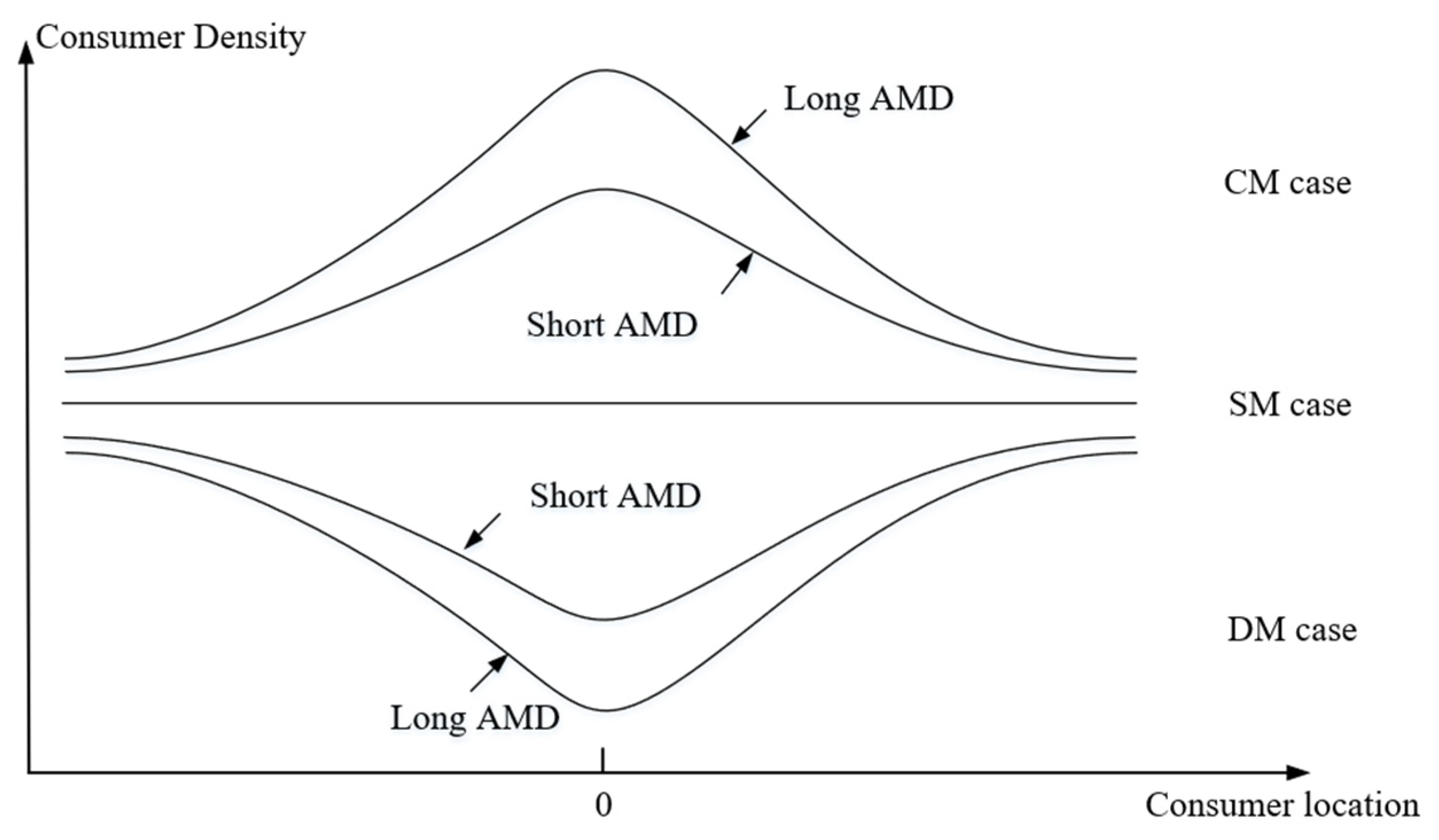
We consider a linear Hotelling city comprised of a firm (located at 0-point) and a continuum of consumers (see Figure 1). Referring to Hernández-García [60], we regard a consumer’s location (denoted by x) in the Hotelling city as his/her physical location in practice. Consumers may move in the Hotelling city, hence their distribution is changeable. Moreover, we assume that the city is boundless, i.e., $x\in (-\infty ,+\infty )$. This enables us to focus on an interesting case in which the market is partially covered. Theoretically, all the consumers in the city, even those at very distant locations, are likely to reach the firm’s vicinity.

To characterize consumer mobility, we consider two discrete periods. In period 1, the consumers have a certain initial distribution in the Hotelling city. Without loss of generality, we assume that they are evenly distributed in the city with density 1. Note that many geographers and economists have developed hypothetical systems of economic areas based on even population distribution [61]. We follow this traditional assumption as it makes the model tractable and helps generate useful insights. In period 2, each consumer makes a random movement from his/her initial location to another. This means that the consumer distribution in period 2 may be different from that in period 1. Essentially, a consumer’s movement is regarded as his/her proactive behavior for non-purchasing purposes, e.g., working, visiting parks, and so on. Therefore, it is independent of the firm’s pricing and advertising strategies.

In practice, consumer distribution changes continuously over time. We can think of this as infinite discrete periods with each period lasting for a short enough time. In this sense, the changes in pricing and advertising strategies from period 1 to period 2 can be interpreted as a representative strategic adjustment occuring due to consumer mobility. Therefore, although our analysis is based on a discrete setting, the results may also be applicable to dynamic decision-making to some extent.

Furthermore, a consumer’s movement in period 2 is described by two attributes, i.e., movement distance and movement direction. A consumer’s movement distance is assumed to be in accordance with the Lévy-walks pattern [5,14,16,25], that is, the movement distance of each consumer follows an identical power-law distribution of $P(\Delta x)={(\Delta x+x_0)}^{-\beta }$, where $1<\beta <2$ and $x_0>0$. Specifically, ${(\Delta x+x_0)}^{-\beta }$ captures the probability of a consumer moving $\Delta x$. Here, $x_0$ is a constant that satisfies ${\displaystyle {\int }_0^{\infty }P(\xi )}d\xi ={\displaystyle {\int }_0^{\infty }{(\xi +x_0)}^{-\beta }}d\xi =1$. Solving the equation, we obtain $x_0=\exp [\frac{\ln (\beta -1)}{1-\beta }]$.

The parameter $\beta$ can be regarded as a proxy that measures the consumers’ AMD. According to the basic property of a power-law distribution, the theoretical range of $\beta$ is $1<\beta <3$, with a smaller $\beta$ indicating longer AMD. Note that the $\beta$ values estimated by Brockmann et al. [5], Gonzalez et al. [14], and Song et al. [16] are 1.59, 1.75, and 1.55, respectively, all smaller than 2. Therefore, we set the range of $\beta$ at $1<\beta <2$, which accommodates to the specific feature of human mobility and guarantees tractability of the model at the same time. In practice, $\beta$ (or AMD) is related to consumers’ activity habits in a certain city. For example, the daily travel distances of Angelenos are two times greater than those of New Yorkers [7]. In addition, $\beta$ may be influenced by some random factors. For instance, people may have smaller activity scopes, i.e., shorter AMD, in snowy or rainy days when road conditions are bad. In the same manner, the emergence of COVID-19 in recent years has limited people’s outdoor activities, thus leading to a sharp reduction in their AMD or a significant increase in $\beta$.

In period 2, a consumer’s movement direction is either moving towards or departing from the firm (see Figure 1). We use parameter $\tau \in [0,1]$ to denote the probability of a consumer moving towards the firm. Correspondingly, $1-\tau$ is the probability of his/her departing from the firm. From the sense of the law of large numbers approximation, $\tau$ (or $1-\tau$) is also the proportion of the consumers that move towards (or depart from) the firm in period 2. Notably, we assume that the firm can rationally anticipate $\beta$ and $\tau$ by observing the consumers’ trajectories in the presence of proximity technologies and make pricing and advertising decisions accordingly. In Section 5.2, we release this assumption by considering the case in which the firm has no idea of the consumers’ distribution in period 2 due to the absence of proximity technologies.

The consumers’ OMT is divided into three patterns according to $\tau$:

(1)

Symmetric movement (SM), $\tau =\frac{1}{2}$, i.e., a half of the consumers move towards the firm and the other half depart from the firm.

(2)

Convergent movement (CM), $\tau >\frac{1}{2}$, i.e., the consumers have an overall tendency to converge to the firm. In other words, more than half of the consumers move towards the firm.

(3)

Divergent movement (DM), $\tau <\frac{1}{2}$, i.e., the consumers have an overall tendency to diverge from the firm. In other words, more than half of the consumers depart away the firm.

3.2. Pricing and Advertising

The firm observes the consumers’ initial distribution in period 1 and rationally anticipates the distribution in period 2. Based on this, the firm sets a uniform product price, p, to the consumers. Meanwhile, it advertises to the consumers and achieves the coverage rate $\varphi \in (0,1)$, which means that a proportion, $\varphi$, of the consumers in the Hotelling city are exposed to advertising and informed of the existence, location, and price of the product. Note that in our setting, the firm’s decision-making in period 2 is independent of that in period 1. This leads to a result in which the firm’s strategies in period 1 are identical to those in period 2 when $\tau =\frac{1}{2}$. Therefore, in the subsequent analysis, we only focus on the firm’s strategies in period 2.

Advertising is costly. Specifically, we assume that the total cost of advertising is $c{\varphi }^2$, where c is a cost coefficient that exogenously depends on the media type or advertising technology. The quadratic cost function is widely used in advertising economics research studies such as Soberman [18], Zhang et al. [23], Zhang et al. [52], and Wang et al. [62]. The convexity of cost function reflects the fact that some consumers are harder to reach than others, that is, a firm has to pay a marginally increasing effort to increase the advertising coverage rate.

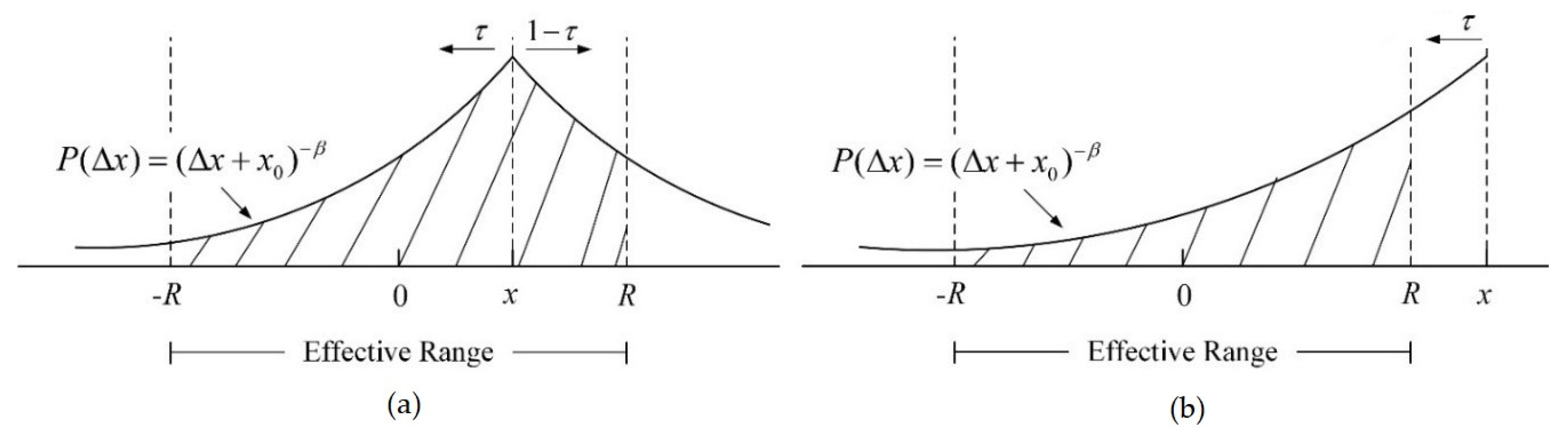
3.3. Consumers’ Purchasing Decisions

In line with classical literature on informative advertising, we assume that the consumers are initially unaware of the product. They do not search for the product’s information if they do not know its existence. As a result, they can learn about the firm’s product information only via advertising. This assumption applies to markets of, for example, new products and niche products that have low awareness and high search costs.

An informed consumer will purchase the product if his/her utility is positive. Particularly, we assume that a consumer whose distance from the firm is x will incur a travel cost, $tx$, to reach the firm. Moreover, he/she obtains a utility, $U=v-p-tx$, from the product, where p, v, and t correspond to the product price, product base value, and unit travel cost, respectively. The consumers are homogeneous in v and t. In addition, to ease exposition, we denote the consumers with positive utility as “effective consumers”. Correspondingly, we define the region in which effective consumers are located as the “effective range (see Figure 1)”. Effective range can be interpreted as a “fence” in the context of geofencing advertising as we have mentioned in Section 1.

Explanations of the notations and subscripts used in this paper are summarized in

Table 1. Explanations of the notations.

Notation	Explanation
$v$	Product base value
t	Unit travel cost
$\tau$	Probability of a consumer moving towards the firm
c	Cost coefficient of advertising
p	Product price
$\beta$	Coefficient indicating AMD
$\pi$	Firm profit
R	Radius of the effective range
$\varphi$	Advertising coverage rate
CS	Consumer surplus
G	Expected number of effective consumers
W	Social welfare

and

Table 2. Explanations of the subscripts.

Subscript	Explanation
n	The case without proximity technologies
c	CM case
s	SM case
d	DM case
k	$k\in \{c,s,d\}$
L	Long-AMD case
S	Short-AMD case

.

4. Results

4.1. Pricing and Advertising Strategies

The number of effective consumers in period 2 is a critical argument for the firm’s pricing and advertising decisions. Therefore, we first formulate it by a G-function and offer some properties of it.

4.1.1. The Number of Effective Consumers

In period 2, the expected number of effective consumers is

$$\begin{array}{l}G(R)=\underset{1}{\underbrace{2{\displaystyle {\int }_0^R[\tau {\displaystyle {\int }_0^{x+R}{(\xi +x_0)}^{-\beta }d\xi }+(1-\tau ){\displaystyle {\int }_0^{R-x}{(\xi +x_0)}^{-\beta }d\xi ]dx}}}}+\underset{2}{\underbrace{2{\displaystyle {\int }_R^{\infty }[\tau {\displaystyle {\int }_{x-R}^{x+R}{(\xi +x_0)}^{-\beta }d\xi }}]dx}}\\ \hspace{1em}\hspace{1em}=2R+\underset{3}{\underbrace{\frac{2(2\tau -1)[x_0^{2-\beta }-{(R+x_0)}^{2-\beta }]}{(1-\beta )(2-\beta )}}}\end{array}$$

(1)

In Equation (1), x is the initial location of a specific consumer and R is the radius of the effective range. Term 1 is the expected number of effective consumers whose initial locations are $x<R$. Term 2 is the expected number of effective consumers whose initial locations are $x>R$. Term 3 captures the increment in effective consumers due to CM or DM. It can be easily proved that term 3 is positive when $\tau >1/2$ and negative when $\tau <1/2$, which is consistent with the intuition that CM (DM) increases (decreases) the number of effective consumers.

Lemma 1.

The G-function monotonically increases with R. Moreover, it marginally diminishes with R in the CM case but marginally increases with R in the DM case. Mathematically,$G^{\prime }(R)\{\begin{array}{l}\in (2,4),\hspace{1em}if\tau >1/2\\ =2,\hspace{1em}\hspace{1em}if\tau =1/2\\ \in (0,2),\hspace{1em}if\tau <1/2\end{array}$and$G^{″}(R)\{\begin{array}{l}<0,\hspace{1em}if\tau >1/2\\ =0,\hspace{1em}if\tau =1/2\\ >0,\hspace{1em}if\tau <1/2\end{array}$.

Proof.

See Appendix A. □

$G^{\prime }(R)>0$ means that the firm can increase the number of effective consumers by widening the effective range or reducing the product price because a consumer is more likely to enter a wider effective range. Moreover, such an effect is weakened (strengthened) when R increases in the CM (DM) case. The intuitions are as follows. In the CM case, the consumers converge to the firm, hence consumer density becomes sparser as R increases (see Figure 2). This means that it becomes harder for the firm to enlarge $G(R)$ by increasing R, which yields ${G^{″}}_c(R)<0$. On the contrary, in the DM case, consumer density becomes thicker as R increases (see Figure 3), which yields ${G^{″}}_d(R)>0$.

Lemma 2.

The number of effective consumers in the CM (DM) case increases (decreases) with AMD, i.e.,$G_{cL}(R)>G_{cS}(R)$and$G_{dL}(R)<G_{dS}(R)$. Moreover, longer AMD renders the G-function increase with R faster in the CM case but slower in the DM case, i.e.,${G^{\prime }}_{cL}(R)>{G^{\prime }}_{cS}(R)>0$and${G^{\prime }}_{dS}(R)>{G^{\prime }}_{dL}(R)>0$.

Proof.

See Appendix A. □

Lemma 2 unveils the effect of the consumers’ AMD on consumer distribution. When the consumers have longer AMD, more of them are expected to reach the firm’s vicinity in the CM case. Hence, there is $G_{cL}(R)>G_{cS}(R)$. Conversely, more consumers will leave from the firm’s vicinity with longer AMD in the DM case, which yields $G_{dL}(R)<G_{dS}(R)$. In addition, a certain increment in R enlarges the number of effective consumers to a greater (smaller) extent if consumers have longer AMD in the CM (DM) case, i.e., ${G^{\prime }}_{cL}(R)>{G^{\prime }}_{cS}(R)$ and ${G^{\prime }}_{dL}(R)<{G^{\prime }}_{dS}(R)$.

Next, we consider the firm’s optimal pricing and advertising decisions. Notably, CM and DM are opposites in terms of definition, which implies that they influence the market outcomes in opposing ways. Therefore, to ease exposition, we mainly focus on the outcomes in the CM case in the main body of the analysis. As a supplement, we offer the outcomes in the DM case in Section 5.1.

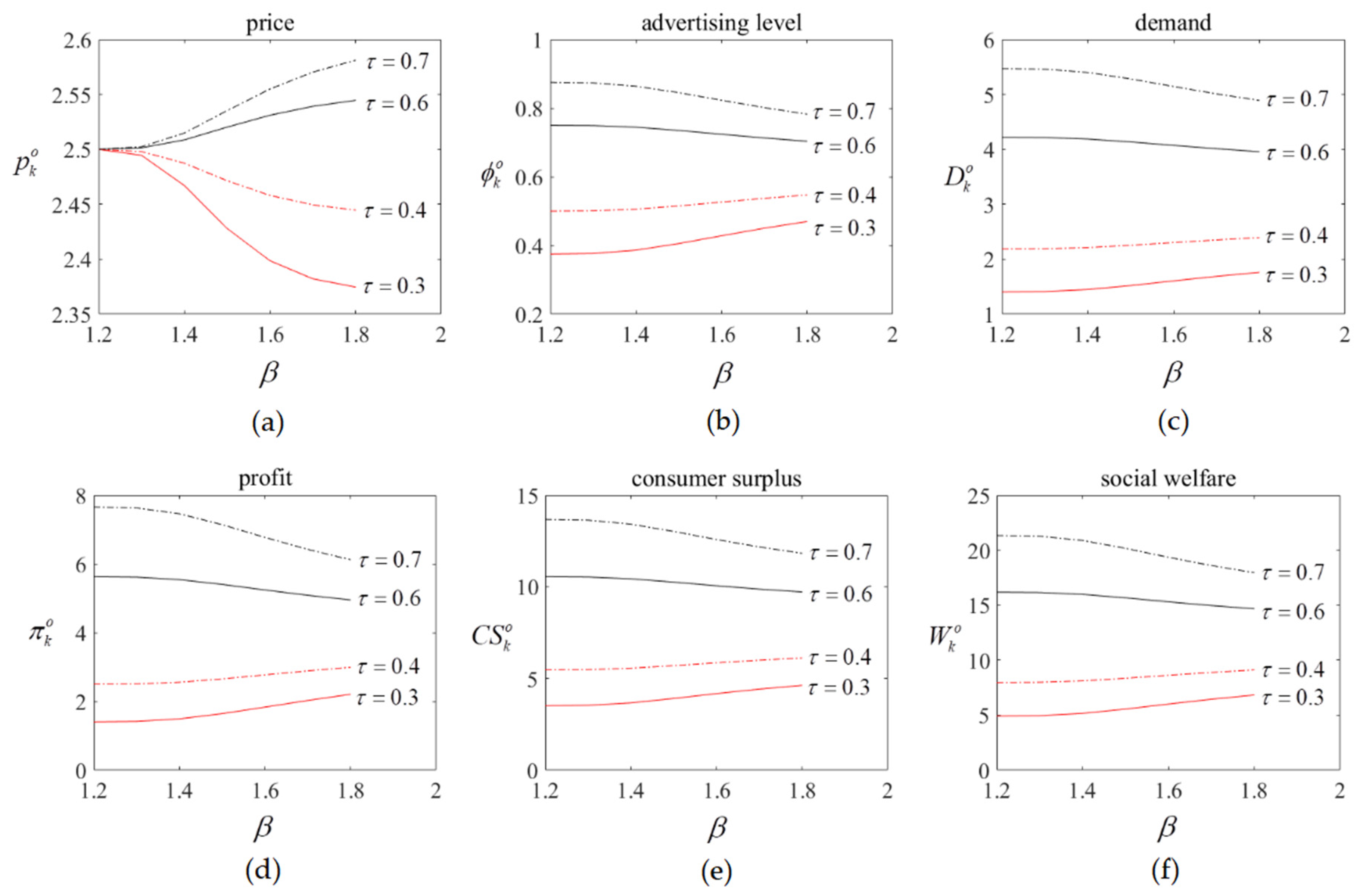
4.1.2. Optimal Decisions

The radius of the effective range is $R_k=\frac{v-p_k}{t}$. Then, the firm’s expected demand and profit are

$$D_k={\varphi }_k{G}_k(\frac{v-p_k}{t})\mathrm{and}$$

(2)

$${\pi }_k=p_k{\varphi }_k{G}_k(\frac{v-p_k}{t})-c{\varphi }_k^2.$$

(3)

Based on Lemma 1, we can obtain

$$\frac{{\partial }^2{\pi }_k}{\partial p_k^2}={\varphi }_k[-\frac{2}{t}{G^{\prime }}_k(\frac{v-p_k}{t})+\frac{p_k}{t^2}{G^{″}}_k(\frac{v-p_k}{t})]<0,\mathrm{where}k\in \{s,c\},$$

(4)

which implies that ${\pi }_k$ is concave with respect to $p_k$. Furthermore, the first order condition yields

$$G_k(\frac{v-p_k}{t})-\frac{p_k}{t}{G^{\prime }}_k(\frac{v-p_k}{t})=0.$$

(5)

The concavity of ${\pi }_k$ ensures that Equation (5) has a unique solution. Let ${\tilde{p}}_k$ denote the solution. The optimal decisions are $p_k^o={\tilde{p}}_k$ and ${\varphi }_k^o=\frac{{\tilde{p}}_k}{2c}{G}_k(\frac{v-{\tilde{p}}_k}{t})$. The corresponding profit is ${\pi }_k^o=\frac{{\tilde{p}}_k^2}{4c}{G}_k^2(\frac{v-{\tilde{p}}_k}{t})$. Particularly, we can present the optimal outcomes in the SM case explicitly, i.e., $p_s^o=\frac{v}{2}$, ${\varphi }_s^o=\frac{v^2}{4ct}$, ${\pi }_s^o=\frac{v^4}{16c{t}^2}$, $C{S}_s^o=\frac{v^4}{8c{t}^2}$, and $W_s^o=\frac{3v^4}{16c{t}^2}$.

4.2. The Effects of Consumer Mobility

In this subsection, we examine the effects of consumer mobility in depth. By comparing the outcomes between CM and SM cases, we disclose the effects of CM in the propositions below.

4.2.1. The Convergent Effect

Proposition 1.

The firm increases its product price and advertising level when the consumers have a stronger tendency to converge to it. Specifically, $p_c^o>p_s^o$and${\varphi }_c^o>{\varphi }_s^o$.

Proof. 

See Appendix A. □

Proposition 1 sheds light on the effect of the consumers’ OMT on the firm’s pricing and advertising strategies, which is defined as the “convergent effect”. A stronger convergent tendency of the consumers makes the firm less incentivized to attract consumers by reducing price or widening the effective range. Therefore, the firm tends to raise the product price in order to gain a higher margin, which is further transferred to advertising investment and raises the advertising level as a result.

Proposition 1 provides advisable guidance to firms on how to adjust pricing and advertising strategies according to changes in consumers’ OMT. Note that reducing price (price promotion) and increasing adverting level (advertising promotion) are two typical ways to stimulate demand in practice. The results of Proposition 1 suggest that firms should concentrate on one of the promotional ways when consumers’ OMT changes. Specifically, as consumers have a stronger convergent tendency, a firm should favor advertising promotion more than price promotion. For example, it can increase advertising intensity at peak times when consumers have convergent tendencies and provide price discounts at off-peak times when consumers have divergent tendencies.

Lemma 3.

The firm gains a higher demand when the consumers have a stronger tendency to converge to it, i.e.,$D_c^o>D_s^o$.

Proof. 

See Appendix A. □

Lemma 3 shows that, when the consumers have a stronger convergent tendency, the firm eventually gains a higher demand even though it increases product price and narrows the effective range. The result presents an insight on firms’ pricing adjustment. Note that consumers’ convergence encourages a firm to increase product price, as Proposition 1 demonstrates. However, a firm needs to bear in mind that the rise in product price should be moderate, thus ensuring an increase in sales or demand. Otherwise, a too sharp rise in product price that reduces demand would harm profitability even in the CM case.

Proposition 2.

When the consumers have a stronger convergent tendency, social welfare increases, i.e., $W_c^o>W_s^o$. Meanwhile, both the firm and consumers become better-off, i.e.,${\pi }_c^o>{\pi }_s^o$and$C{S}_c^o>C{S}_s^o$.

Proof. 

See Appendix A. □

Proposition 2 ascertains the effect of the consumers’ OMT on social welfare. Interestingly, although the firm raises product price in the CM case, reducing an individual consumer’s surplus, the consumers obtain higher surplus overall. A plausible reason is that in the CM case, more consumers enter the effective range and have a chance to enjoy the utility of the product. This positive impact dominates the negative impact from a higher product price. Meanwhile, the firm has a higher demand and product price at the same time under the optimal strategies. As a result, it benefits from the consumers’ CM.

4.2.2. The Scaling Effect

Essentially, the convergent effect of consumer mobility reflects the role of parameter $\tau$. In the following proposition, we show the role of the other critical parameter $\beta$.

Proposition 3.

The firm increases its advertising level but decreases its product price when the consumers have longer AMD in the CM case. Mathematically,${\varphi }_{cL}^o>{\varphi }_{cS}^o$and$p_{cL}^o<p_{cS}^o$.

Proof. 

See Appendix A. □

Propositions 3 reveals an interesting finding that the consumers’ AMD has opposing influences in the firm’s pricing and advertising strategies. Specifically, longer AMD strengthens the convergent effect of consumers’ OMT on advertising strategy but weakens that on pricing strategy. In other words, when consumers have longer AMD, the firm will have a stronger incentive to increase the adverting level but a weaker incentive to increase product price in the CM case.

Proposition 3 provides a useful insight that a firm should attach attention not only to consumers’ OMT but also to consumers’ AMD. In particular, the scaling effect implies that the adjustment magnitude of the advertising level should be greater, whereas the adjustment magnitude of the product price should be smaller with longer AMD. In other words, a firm’s advertising (pricing) strategy should be more (less) elastic with longer AMD. In practice, consumers’ AMD is closely related to their activity habits and the transportation conditions of their cities. Therefore, a firm is suggested to adopt differentiated strategies in its branch stores located in different cities, if it has any, according to the specific movement patterns of the cities’ residents. Specifically, the stores in long-AMD cities should implement elastic advertising strategies, whereas the stores in short-AMD cities should implement elastic pricing strategies, to cope with the changes in consumers’ OMT. In addition, in the current COVID-19 era, consumers’ AMD has changed more violently than ever before. This means that consumers’ AMD has more significant impacts on firms’ strategies. The results of Proposition 3 may be helpful for firms to cope with these challenges.

Proposition 4.

When the consumers have longer AMD, the firm becomes better-off in the CM case, i.e.,${\pi }_{cL}^o>{\pi }_{cS}^o$.

Proof. 

See Appendix A. □

Proposition 4 shows that longer AMD magnifies the convergent effect of consumers’ OMT on profitability. The consumers with longer AMD have a more significant convergent tendency in the CM case, as Lemma 2 shows. Then, longer AMD results in a higher product price and demand at the same time, thus enhancing the firm’s profitability. Conversely, Proposition 4 implies that firms located in longer-AMD cities tend to suffer from a larger fluctuation in their profit performances across time, which brings potential challenges to their management of capacity, store staffing, inventory, etc. Therefore, it is suggested that a firm should carefully consider consumer mobility in marketing and operational planning, especially when the city residents’ AMD is long.

5. Extensions and Discussions

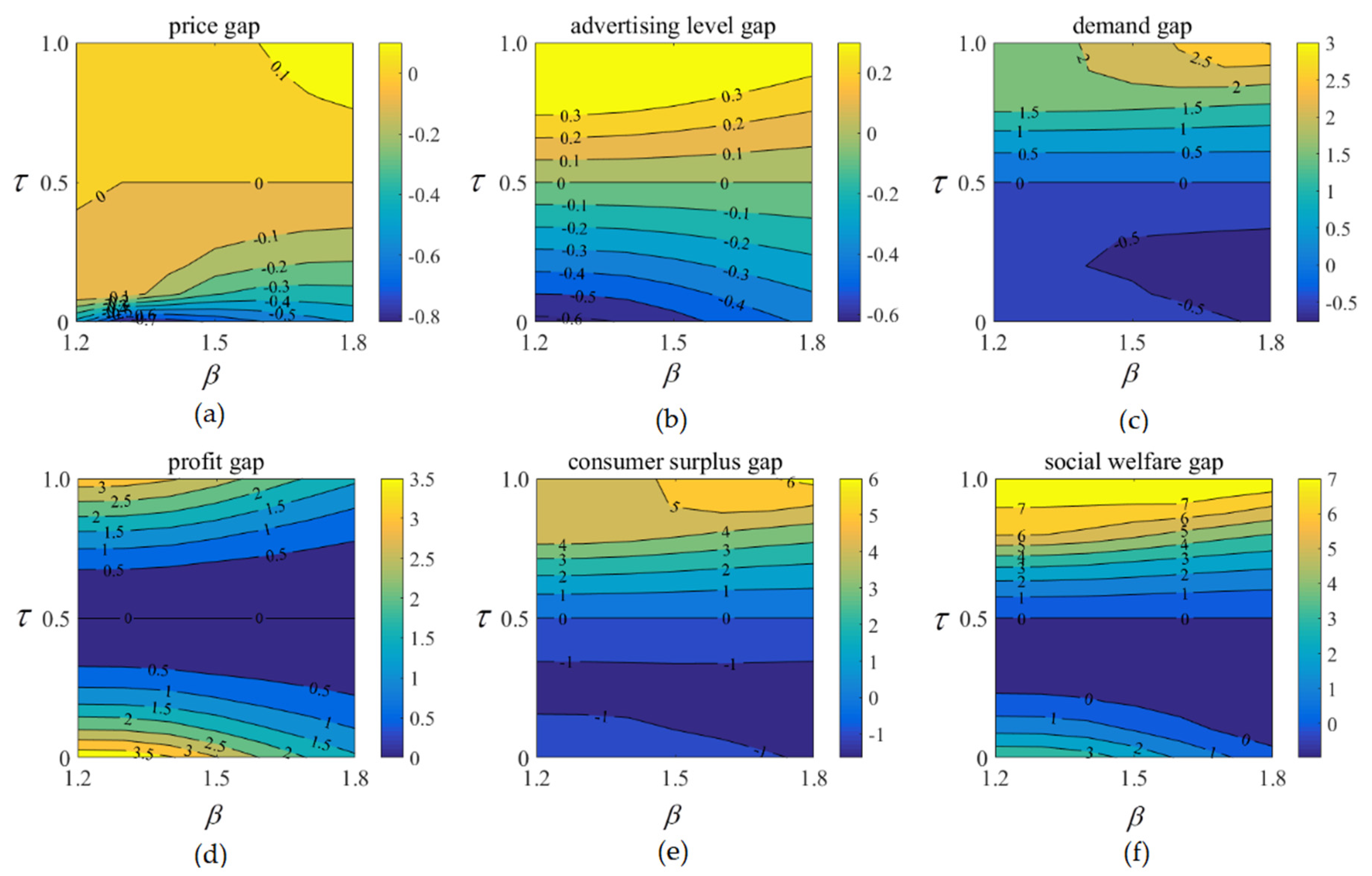
5.1. The DM Case

Intuitively, DM is a reverse process to CM. Therefore, the effects of DM should be opposing to those of CM. We explore this intuition in this subsection. Note that in the DM case, concavity of the profit function can hardly be proved analytically due to the complexity of the model. Therefore, we derive the effects of DM analytically under an assumption that the profit function is concave in the DM case. As a supplement, we use numerical examples to check the robustness of the analytical results. The effects of DM are shown in the following corollaries.

Corollary 1.

The divergent effect:

(1) 

The firm decreases its product price and advertising level when the consumers have a stronger tendency to diverge from it, i.e.,$p_d^o<p_s^o$and${\varphi }_d^o<{\varphi }_s^o$.

(2) 

The firm gains a lower demand when the consumers have a stronger tendency to diverge from it, i.e.,$D_d^o<D_s^o$.

(3) 

When the consumers have a stronger tendency to diverge from the firm, social welfare decreases, i.e.,$W_d^o<W_s^o$. Meanwhile, both the firm and consumers become worse-off. Mathematically,${\pi }_d^o<{\pi }_s^o$and$C{S}_d^o<C{S}_s^o$.

Proof. 

See Appendix A. □

Corollary 2.

The scaling effect:

(1) 

The firm decreases its advertising level but increases its product price when the consumers have longer AMD in the DM case, i.e.,${\varphi }_{dL}^o<{\varphi }_{dS}^o$and$p_{dL}^o>p_{dS}^o$.

(2) 

When the consumers have longer AMD, the firm becomes worse-off in the DM case, i.e.,${\pi }_{dL}^o<{\pi }_{dS}^o$.

Proof. 

See Appendix A. □

The results of Corollaries 1 and 2 indicate that DM leads to reverse outcomes relative to CM. Furthermore, the results of the numerical analysis are illustrated in Figure 3. The numerical results validate the robustness of the main results obtained analytically. In addition, they present several additional insights about the scaling effect of the consumers’ AMD on social welfare.

In the examples, we set $v=5$, $t=1$, $c=10$, $\tau \in \{0.3,0.4,0.6,0.7\}$, and $\beta \in \{1.2,1.3,1.4,1.5,1.6,1.7,1.8\}$. The coefficient c satisfies ${\varphi }_b^o=\frac{v^2}{4ct}<1$. We calculate the optimal solutions through genetic algorithms, not requiring concave objective functions.

In Figure 3, the curves with greater $\tau$ values (e.g., $\tau =0.7$) are above those with smaller $\tau$ values (e.g., $\tau =0.6$). This corroborates the convergent (or divergent) effect of consumer mobility. In addition, the gap between the CM case curves (e.g., $\tau =0.6$) and DM case curves (e.g., $\tau =0.4$) is narrower when $\beta$ decreases in Figure 3a but widens when $\beta$ decreases in Figure 3b. This confirms our previous finding that longer AMD weakens the convergent effect of consumers’ OMT on price but strengthens that on advertising level. Moreover, Figure 3c–f show that longer AMD also magnifies the convergent effect of the consumers’ OMT on firm demand, firm profit, consumer surplus, and social welfare, respectively.

5.2. The Case without Proximity Technologies

In Section 4, we explore the effects of consumer mobility given that the firm is capable of tracing and anticipating consumer location due to proximity technologies. In this subsection, we consider the case without proximity technologies. That is, the firm only knows the consumer distribution in period 1 but has no information on the consumer distribution in period 2. For example, a firm knows the fixed addresses of its potential consumers in the city but may not know where they would be at the real-time of advertising. By comparing the outcomes with and without proximity technologies, we can unveil the effects of the presence of proximity technologies on the market outcomes.

Without proximity technologies, the firm makes pricing and advertising strategies according to the consumer distribution in period 1. It is easy to obtain the optimal decisions $p_n^o=\frac{v}{2}$ and ${\varphi }_n^o=\frac{v^2}{4ct}$, which are mathematically identical to those in the SM case. Based on the results of Proposition 1 and Corollary 1, we can easily prove that $p_c^o>p_s^o=p_n^o>p_d^o$ and ${\varphi }_c^o>{\varphi }_s^o={\varphi }_n^o>{\varphi }_d^o$.

Furthermore, it is noteworthy that the decisions are made according to the distribution in period 1 but the realized demands and profits are finally dependent upon the real distribution in period 2. To analyze this, let $D_{n,k}^o$ and ${\pi }_{n,k}^o$ denote the realized demands and profits without proximity technologies in case $k$, where $k\in \{c,s,d\}$. Then, we have

$$D_{n,k}^o={\varphi }_n^o{G}_k(\frac{v-p_n^o}{t})=\frac{v^2}{4ct}{G}_k(\frac{v}{2t})\mathrm{and}$$

(6)

$${\pi }_{n,k}^o=p_n^o{D}_{n,k}^o-c{({\varphi }_n^o)}^2=\frac{v^3}{8ct}{G}_k(\frac{v}{2t})-\frac{v^4}{16c{t}^2}.$$

(7)

Considering proximity technologies enable the firm to adjust its strategies dynamically with changes in market environment, the correctness of the strategies is enhanced. As a result, the firm’s profitability is improved by proximity technologies in both CM and DM cases. Mathematically, ${\pi }_k^o={\pi }_k(p_k^o,{\varphi }_k^o)\ge {\pi }_k^{}(p_n^o,{\varphi }_n^o)={\pi }_{n,k}^o$.

The consumers’ surpluses with and without proximity technologies are

$$C{S}_k^o=\underset{1}{\underbrace{(v-p_k^o)G_k^{}(\frac{v-p_k^o}{t})}}\cdot \underset{2}{\underbrace{{\varphi }_k^o}}\mathrm{and}$$

(8)

$$C{S}_{n,k}^o=\underset{1}{\underbrace{(v-p_n^o)G_k^{}(\frac{v-p_n^o}{t})}}\underset{2}{\underbrace{\cdot {\varphi }_n^o}}.$$

(9)

Term 1 in each equation measures the maximum surplus that effective consumers are likely to have. Term 2 measures the proportion of effective consumers that finally enjoy the surplus. Notably, the presence of proximity technologies has opposing effects on term 1 and term 2. For example, in the CM case, the maximum surplus of effective consumers becomes smaller in the presence of proximity technologies since $p_c^o>p_n^o$. However, ${\varphi }_c^o>{\varphi }_n^o$ indicates that a larger proportion of effective consumers enjoy the surplus. Therefore, the overall effect of proximity technologies on consumer surplus is obscure.

To ascertain the effect, we conduct a numerical analysis that examines the gaps between the outcomes with and without proximity technologies. Akin to Section 5.1, we set $v=5$, $t=1$, $c=10$, $\tau \in \{0,0.1,0.2,0.3,0.4,0.5,0.6,0.7,0.8,0.9,1.0\}$, and $\beta \in \{1.2,1.3,1.4,1.5,1.6,1.7,1.8\}$. The results are illustrated in Figure 4.

We can see in Figure 4e that the presence of proximity technologies increases consumer surplus in the CM case but decreases consumer surplus in the DM case, which implies that the effect of proximity technologies on term 2 offset that on term 1 in Equations (8) and (9). In other words, the presence of proximity technologies influences consumer surplus through affecting advertising strategy more significantly than through affecting pricing strategy. More interestingly, although the presence of proximity technologies decreases consumer surplus in the DM case, it increases social welfare if $\beta$ is small enough (see Figure 4f); that is, if consumers have long enough AMD, the presence of proximity technologies can benefit the whole society even in the DM case. This result reveals that introducing new technologies such as proximity technologies may be an effective way to revitalize an ailing industry that suffers from consumer loss.

In addition, in line with the spirit of Proposition 3, $\beta$ affects the price gap and advertising level gap in opposing ways. For example, smaller $\beta$ narrows the price gap but widens the advertising level gap (see Figure 4a,b), which means that the presence of proximity technologies becomes more influential in advertising strategy but less influential in pricing strategy if consumers have longer AMD. This suggests that firms located in long-AMD cities should make relatively major adjustments in their advertising strategies but relatively minor adjustments in their pricing strategies after adopting proximity technologies. In addition, Figure 4d shows that longer AMD magnifies the profit gap. This result implies that, by adopting proximity technologies, firms located in long-AMD cities may achieve more significant improvements in profitability than those located in short-AMD cities. In consequence, firms in long-AMD cities may have stronger incentives to introduce new technologies than firms in short-AMD cities.

5.3. The Firm’s Under-Advertising Behavior

We arrive at another interesting finding that consumer mobility is influential in the firm’s under-advertising behavior. We refer to the ratio of “the advertising level set by the firm” to “the advertising level maximizing the social welfare” as a proxy that reflects the extent of under-advertising. A ratio that is smaller (greater) than 1 indicates under-advertising (over-advertising).

The social welfare is the sum of the firm’s profit and consumers’ surplus, which is described as follows:

$$W_k=v{\varphi }_k{G}_k(\frac{v-p_k}{t})-c{\varphi }_k^2.$$

(10)

Then, by solving the first order condition, we obtain the socially optimal advertising level ${\varphi }_k^{so}=\frac{v{G}_k(\frac{v-p_k^o}{t})}{2c}$. Recall that the advertising level set by the firm is ${\varphi }_k^o=\frac{p_k^o}{2c}{G}_k(\frac{v-p_k^o}{t})$. Therefore, it can be easily obtained that $\frac{{\varphi }_k^o}{{\varphi }_k^{so}}=\frac{p_k^o}{v}<1$, which reveals the firm’s under-advertising behavior.

Proposition 5.

The firm provides a lesser amount of advertising than what is needed to maximize social welfare. Moreover, a stronger convergent tendency of the consumers suppresses the firm’s under-advertising incentive and such a suppressing effect is weakened by longer AMD.

Proof. 

Proposition 1 indicates that $p_c^o>p_d^o$, which yields $\frac{{\varphi }_d^o}{{\varphi }_d^{so}}<\frac{{\varphi }_c^o}{{\varphi }_c^{so}}$, i.e., the firm’s under-advertising incentive is weaker in the CM case than in the DM case. In addition, Proposition 3 shows that $p_{cL}^o<p_{cS}^o$ and $p_{dL}^o>p_{dS}^o$. Hence, it can be obtained that $\frac{{\varphi }_{cL}^o}{{\varphi }_{cL}^{so}}<\frac{{\varphi }_{cS}^o}{{\varphi }_{cS}^{so}}$ and $\frac{{\varphi }_{dL}^o}{{\varphi }_{dL}^{so}}>\frac{{\varphi }_{dS}^o}{{\varphi }_{dS}^{so}}$. This means that the firm’s under-advertising incentive is stronger with longer AMD in the CM case but weaker with longer AMD in the DM case. □

6. Conclusions

6.1. Summary of the Main Findings

Rapid development of proximity technologies and pervasive usage of mobile devices enable firms to obtain abundant consumer location information, which has profound influences in firms’ marketing and operations strategies. This paper incorporates consumer mobility, i.e., consumers’ Lévy-walking behavior, into advertising economics models, thereby providing a novel method for studying the economic effects of consumer mobility on pricing and advertising strategies. We establish an analytical model that captures two key attributes of consumer mobility, i.e., OMT and AMD.

Our findings provide useful implications on developing pricing and advertising strategies according to consumer mobility. We unveil the convergent effect of consumers’ OMT. It shows that product price and advertising level both raise when consumers have a stronger tendency to converge to a firm. Moreover, consumers’ convergence improves social welfare by increasing both firm profit and consumer surplus. Furthermore, we disclose the scaling effect of consumers’ AMD. Interestingly, we find that consumers’ AMD has opposing impacts on a firm’s pricing and advertising strategies. Specifically, longer AMD strengthens the convergent effect of OMT on advertising strategy but weakens that on pricing strategy.

In addition, we uncover the impacts of the emergence of proximity technologies through a numerical analysis. The results reveal that the presence of proximity technologies increases consumer surplus in the CM case but decreases that in the DM case. Interestingly, the emergence of proximity technologies may improve social welfare even in the DM case as long as consumers’ AMD is long enough. Finally, we examine a firm’s under-advertising behavior from the perspective of consumer mobility. The result shows that consumers’ convergence suppresses a firm’s under-advertising incentive and such a suppressing effect is weakened by longer AMD.

Although this paper does not cover all the complex aspects of the reality, it provides several enlightening management and economics insights. Most importantly, it is a meaningful attempt to model consumer mobility in a marketing-operations context. The mathematical properties of the G-function (given by Lemmas 1 and 2) reflect core features of demand functions with respect to consumer mobility and offer advisable guidelines to the modeling of future research.

6.2. Limitations and Opportunities for Future Research

There are several limitations of this paper that may be overcome by several extensions in further research. First, our results are based on a monopoly setting. It is meaningful to consider market competition and unveil some additional or new insights when firms have competitive incentives. Under monopolistic conditions, as in this paper, consumers’ convergence increases the product price and advertising level. However, under competitive conditions, a firm may have a stronger incentive to compete for consumers against its rival by reducing price when more consumers enter the market. As a result, consumers’ convergence might decrease the product price or advertising level due to the competitive effect.

Second, it is a possible extension to consider the relationship between consumers’ physical locations and purchasing intentions. In this paper, all the consumers have identical purchase intentions towards the firm’s product, which is measured by the parameter v. However, in practice, consumers’ purchase intentions may vary. Moreover, the previous wisdom on consumer behavior shows that consumers’ locations are indicative of their purchasing intentions. For example, if a consumer is located at a stadium watching a football game, he/she is very likely to have interests in sports products. Then, a firm selling relevant products can send advertisements to the consumer when he/she is at the stadium. In this context, consumers at different locations are heterogenous with respect to v and a firm not only cares about a consumer’s distance from the firm itself but also his/her distance to another landmark.

Third, the utility function of this paper contains only one decision variable, i.e., product price. It might be worthy to introduce some other variables. In particular, as we have mentioned in Section 2.2.1, a firm can increase consumers’ valuation, v, by adding some emotional values, such as happiness and social reputation to its product. Moreover, the added value can be communicated to consumers through advertising, which is known as persuasive advertising [63]. Then, in a persuasive advertising context, a firm determines not only the advertising coverage rate but also the advertising persuasive effort. In other words, it is meaningful to study the interaction between the two advertising variables.

References

1. O’Dea, S. Number of Smartphone Subscriptions Worldwide from 2016 to 2026. 2021. Available online: https://www.statista.com/statistics/330695/number-of-smartphone-users-worldwide (accessed on 5 July 2020).
2. eMarketer. More Marketers Use Proximity Tech, Beacons, to Get Closer to the Action. 2016. Available online: https://www.emarketer.com/Article/More-Marketers-Use-Proximity-Tech-Beacons-Closer-Action/1014428 (accessed on 7 September 2020).
3. eMarketer. What Marketers Need to Know about Smart Cities. 2017. Available online: https://www.emarketer.com/Article/What-Marketers-Need-Know-About-Smart-Cities/1015956 (accessed on 7 September 2020).
4. Ghose, A.; Li, B.; Liu, S. Mobile targeting using customer trajectory patterns. Manag. Sci. 2019, 65, 5027–5049. [Google Scholar] [CrossRef]
5. Brockmann, D.; Hufnagel, L.; Geisel, T. The scaling laws of human travel. Nature 2006, 439, 462–465. [Google Scholar] [CrossRef] [PubMed]
6. Song, C.; Qu, Z.; Blumm, N.; Barabasi, A.L. Limits of predictability in human mobility. Science 2010, 327, 1018–1021. [Google Scholar] [CrossRef] [PubMed] [Green Version]
7. Isaacman, S.; Becker, R.; Cáceres, R.; Kobourov, S.; Rowland, J.; Varshavsky, A. A tale of two cities. Workshop Mob. Comput. Syst. Appl. 2010, 19–24. [Google Scholar] [CrossRef]
8. Luo, X.; Andrews, M.; Fang, Z.; Phang, C.W. Mobile targeting. Manag. Sci. 2014, 60, 1738–1756. [Google Scholar] [CrossRef] [Green Version]
9. Danaher, P.J.; Smith, M.S.; Ranasinghe, K.; Danaher, T.S. Where, when, and how long: Factors that influence the redemption of mobile phone coupons. J. Mark. Res. 2015, 52, 710–725. [Google Scholar] [CrossRef]
10. Fong, N.M.; Fang, Z.; Luo, X.M. Geo-conquesting: Competitive locational targeting of mobile promotions. J. Mark. Res. 2015, 52, 726–735. [Google Scholar] [CrossRef] [Green Version]
11. Kats, R. BestBuy Drives Foot Traffic to Locations via Geofencing Campaign. 2012. Available online: https://www.retaildive.com/ex/mobilecommercedaily/best-buy-drives-foot-traffic-to-locations-via-geofencing-campaign (accessed on 5 July 2020).
12. Tode, C. Location Targeting More Than Doubles Performance of Mobile Ads: Report. 2013. Available online: https://www.marketingdive.com/ex/mobilemarketer/cms/news/research/14731.html (accessed on 5 July 2020).
13. Hotelling, H. Stability in competition. Econ. J. 1929, 39, 41–57. [Google Scholar] [CrossRef]
14. Gonzalez, M.C.; Hidalgo, C.A.; Barabasi, A.L. Understanding individual human mobility patterns. Nature 2008, 453, 779–782. [Google Scholar] [CrossRef]
15. Lee, K.; Hong, S.; Kim, S.; Rhee, I.; Song, C. SLAW: A new mobility model for human walks. IEEE Infocom Int. Conf. Comput. Commun. 2009, 855–863. [Google Scholar] [CrossRef]
16. Song, C.M.; Koren, T.; Wang, P.; Barabasi, A.L. Modelling the scaling properties of human mobility. Nat. Phys. 2010, 6, 818–823. [Google Scholar] [CrossRef] [Green Version]
17. Grossman, G.M.; Shapiro, C. Informative advertising with differentiated products. Rev. Econ. Stud. 1984, 51, 63–81. [Google Scholar] [CrossRef]
18. Soberman, D.A. Research note: Additional learning and implications on the role of informative advertising. Manag. Sci. 2004, 50, 1744–1750. [Google Scholar] [CrossRef] [Green Version]
19. Hamilton, S.F. Informative advertising in differentiated oligopoly markets. Int. J. Ind. Organ. 2009, 27, 60–69. [Google Scholar] [CrossRef] [Green Version]
20. Stahl, D.O. Oligopolistic pricing and advertising. J. Econ. Theor. 1994, 64, 162–177. [Google Scholar] [CrossRef]
21. Stegeman, M. Advertising in competitive markets. Am. Econ. Rev. 1991, 81, 210–223. [Google Scholar]
22. Esteves, R.B. Customer poaching and advertising. J. Ind. Econ. 2009, 57, 112–146. [Google Scholar] [CrossRef]
23. Zhang, J.; Cao, Q.; Yue, X. Target or not? Endogenous advertising strategy under competition. IEEE Trans. Syst. Man Cybern. Syst. 2020, 50, 4472–4481. [Google Scholar] [CrossRef]
24. Noulas, A.; Scellato, S.; Lambiotte, R.; Pontil, M.; Mascolo, C. A tale of many cities: Universal patterns in human urban mobility. PLoS ONE 2012, 7, e37027. [Google Scholar] [CrossRef]
25. Rhee, I.; Shin, M.; Hong, S.; Lee, K.; Kim, S.J.; Chong, S. On the Lévy-walk nature of human mobility. IEEE ACM Trans. Netw. 2011, 19, 630–643. [Google Scholar] [CrossRef]
26. Wesolowski, A.; Eagle, N.; Noor, A.M.; Snow, R.W.; Buckee, C.O. The impact of biases in mobile phone ownership on estimates of human mobility. J. R. Soc. Interface 2013, 10, 20120986. [Google Scholar] [CrossRef] [PubMed]
27. Cuttone, A.; Lehmann, S.; González, M. Understanding predictability and exploration in human mobility. EPJ Data Sci. 2018, 7, 2. [Google Scholar] [CrossRef] [Green Version]
28. Damiani, M.L.; Hachem, F.; Quadri, C.; Rossini, M.; Gaito, S. On location relevance and diversity in human mobility data. ACM Trans. Spat. Algorithms Syst. 2020, 7, 1–38. [Google Scholar] [CrossRef]
29. Hanson, S.; Hanson, P. The travel-activity patterns of urban residents: Dimensions and relationships to sociodemographic characteristics. Econ. Geogr. 1981, 57, 332–347. [Google Scholar] [CrossRef]
30. Hanson, S.; Johnston, I. Gender differences in work-trip length. Urban Geogr. 1985, 9, 180–202. [Google Scholar] [CrossRef]
31. Brahim, N.; Lahmandi-Ayed, R.; Laussel, D. Is targeted advertising always beneficial? Int. J. Ind. Organ. 2011, 29, 678–689. [Google Scholar] [CrossRef]
32. Wang, W.; Li, G.; Fung, Y.K.R.; Cheng, T.C.E. Mobile advertising and traffic conversion: The effects of front traffic and spatial competition. J. Interact. Mark. 2019, 47, 84–101. [Google Scholar] [CrossRef]
33. Mogilner, C. The pursuit of happiness: Time, money, and social connection. Psychol. Sci. 2010, 21, 1348–1354. [Google Scholar] [CrossRef] [Green Version]
34. Mogilner, C.; Aaker, J.; Kamvar, S.D. How happiness affects choice. J. Consum. Res. 2012, 39, 429–443. [Google Scholar] [CrossRef]
35. Alba, J.W.; Williams, E.F. Pleasure principles: A review of research on hedonic consumption. J. Consum. Psychol. 2013, 23, 2–18. [Google Scholar] [CrossRef]
36. Bagozzi, R.P.; Belanche, D.; Casaló, L.V.; Flavián, C. The role of anticipated emotions in purchase intentions. Psychol. Mark. 2016, 33, 629–645. [Google Scholar] [CrossRef]
37. Goldberg, M.E.; Hartwick, J. The effects of advertiser reputation and extremity of advertising claim on advertising effectiveness. J. Consum. Res. 1990, 17, 172–179. [Google Scholar] [CrossRef]
38. Amaldoss, W.; Jain, S. Conspicuous consumption and sophisticated thinking. Manag. Sci. 2005, 51, 1449–1466. [Google Scholar] [CrossRef] [Green Version]
39. Amaldoss, W.; Jain, S. Pricing of conspicuous goods: A competitive analysis of social effects. J. Mark. Res. 2005, 42, 30–42. [Google Scholar] [CrossRef] [Green Version]
40. Cheema, A.; Kaikati, A.M. The effect of need for uniqueness on word of mouth. J. Mark. Res. 2010, 47, 553–563. [Google Scholar] [CrossRef] [Green Version]
41. Yang, L.; Wang, Z.; Hahn, J. Scarcity strategy in crowdfunding: An empirical exploration of reward limits. Inf. Syst. Res. 2020, 31, 1107–1131. [Google Scholar] [CrossRef]
42. Hu, M.; Shi, M.; Wu, J. Simultaneous vs. sequential group-buying mechanisms. Manag. Sci. 2013, 59, 2805–2822. [Google Scholar] [CrossRef]
43. Wu, J.; Shi, M.; Hu, M. Threshold effects in online group buying. Manag. Sci. 2015, 61, 2025–2040. [Google Scholar] [CrossRef] [Green Version]
44. Hu, M.; Milner, J.; Wu, J. Liking and following and the newsvendor: Operations and marketing policies under social influence. Manag. Sci. 2016, 62, 867–879. [Google Scholar] [CrossRef] [Green Version]
45. Doha, A.; Elnahla, N.; McShane, L. Social commerce as social networking. J. Retail. Consum. Serv. 2019, 47, 307–321. [Google Scholar] [CrossRef]
46. Fang, Z.; Gu, B.; Luo, X.; Xu, Y. Contemporaneous and delayed sales impact of location-based mobile promotions. Inf. Syst. Res. 2015, 26, 552–564. [Google Scholar] [CrossRef]
47. Li, C.; Luo, X.; Zhang, C.; Wang, X. Sunny, rainy, and cloudy with a chance of mobile promotion effectiveness. Mark. Sci. 2017, 36, 762–779. [Google Scholar] [CrossRef] [Green Version]
48. Andrews, M.; Luo, X.M.; Fang, Z.; Ghose, A. Mobile Ad Effectiveness: Hyper-Contextual Targeting with Crowdedness. Mark. Sci. 2016, 35, 218–233. [Google Scholar] [CrossRef]
49. Bagwell, K. The economic analysis of advertising. Handb. Ind. Organ. 2007, 3, 1701–1844. [Google Scholar]
50. Butters, G.R. Equilibrium distributions of sales and advertising prices. Uncertain. Econ. 1978, 493–513. [Google Scholar] [CrossRef]
51. Karray, S. Modeling brand advertising with heterogeneous consumer response: Channel implications. Ann. Oper. Res. 2015, 233, 181–199. [Google Scholar] [CrossRef]
52. Zhang, J.Q.; Zhong, W.J.; Mei, S. Competitive effects of informative advertising in distribution channels. Mark. Lett. 2012, 23, 561–584. [Google Scholar] [CrossRef]
53. Ghosh, B.P.; Galbreth, M.R.; Shang, G. The competitive impact of targeted television advertisements using DVR technology. Decis. Sci. 2013, 44, 951–971. [Google Scholar] [CrossRef]
54. Li, L.; Chen, J.; Raghunathan, S. Informative role of recommender systems in electronic marketplaces: A boon or a bane for competing sellers. MIS Q. 2020, 44, 1957–1985. [Google Scholar] [CrossRef]
55. Chen, Y.; Li, X.; Sun, M. Competitive mobile geo targeting. Mark. Sci. 2017, 36, 666–682. [Google Scholar] [CrossRef] [Green Version]
56. Dixit, A.; Norman, V. Advertising and welfare. Bell J. Econ. 1978, 9, 1–17. [Google Scholar] [CrossRef]
57. Tremblay, C.H.; Tremblay, V.J. Advertising, price, and welfare: Evidence from the US brewing industry. South. Econ. J. 1995, 62, 367–381. [Google Scholar] [CrossRef]
58. Becker, G.S.; Murphy, K.M. A simple theory of advertising as a good or bad. Q. J. Econ. 1993, 108, 941–964. [Google Scholar] [CrossRef]
59. Stivers, A.; Tremblay, V.J. Advertising, search costs, and social welfare. Inf. Econ. Policy 2005, 17, 317–333. [Google Scholar] [CrossRef]
60. Hernández-García, J.M. Informative advertising, imperfect targeting and welfare. Econ. Lett. 1997, 55, 131–137. [Google Scholar] [CrossRef]
61. Losch, A. The economics of location. Economica. 1956, 23, 175. [Google Scholar]
62. Wang, R.; Gou, Q.; Choi, T.M.; Liang, L. Advertising strategies for mobile platforms with “apps”. IEEE Trans. Syst. Man Cybern. Syst. 2016, 48, 767–778. [Google Scholar] [CrossRef]
63. Wu, C.; Chen, Y.; Wang, C. Is persuasive advertising always combative in a distribution channel? Mark. Sci. 2009, 28, 1157–1163. [Google Scholar] [CrossRef]
Figure 1. The market and a consumer’s movement: (a) A consumer’s movement when his/her location is x < R ; (b) A consumer’s movement when his/her location is x > R .
Jtaer 16 00119 g001
Figure 2. Consumer distribution with respect to OMT.
Jtaer 16 00119 g002
Figure 3. The effects of consumer mobility on the market outcomes: (a) the effect on price; (b) the effect on advertising level; (c) the effect on demand; (d) the effect on profit; (e) the effect on consumer surplus; and (f) the effect on social welfare.
Jtaer 16 00119 g003
Figure 4. Contour plots on the effects of proximity technologies: (a) the effect on the price gap; (b) the effect on the advertising level gap; (c) the effect on the demand gap; (d) the effect on the profit gap; (e) the effect on the consumer surplus gap; and (f) the effect on the social welfare gap.
Jtaer 16 00119 g004