Article

A Dynamic Contest Model of Platform Competition in Two-Sided Markets

1
School of Business, Lucerne University of Applied Sciences and Arts, 6002 Luzern, Switzerland
2
Institute of Sport Sciences, University of Lausanne, 1015 Lausanne, Switzerland
3
Department of Business Administration, University of Zurich, 8006 Zurich, Switzerland
*
Author to whom correspondence should be addressed.
J. Theor. Appl. Electron. Commer. Res. 2021, 16(6), 2091-2109; https://doi.org/10.3390/jtaer16060117
Submission received: 17 June 2021 / Revised: 11 August 2021 / Accepted: 13 August 2021 / Published: 18 August 2021

Abstract

:
This paper examines the dynamic competition between platform firms in two-sided markets with network externalities. In our model, two platforms compete with each other via a contest to dominate a certain market. If one platform wins the contest, it can serve the market for a certain duration as a monopolistic platform. Our paper shows that platform firms can compensate for cost disadvantages with network effects. A head start (e.g., technological advantage) does not guarantee future success for platform firms. Network effects and cost efficiency are decisive for future success. Interestingly, higher costs of a platform can induce higher platform profits in our dynamic model. Moreover, we find that a platform’s size and profit are not necessarily positively correlated. Our model also provides new insights with respect to the underlying causes for the emergence of market dominance. The combination of technological carry-over and network effects can explain a long-lasting dominance of a platform that benefits from a head start. The necessary preconditions for this emergence are convex costs, small network effects and high carry-over.

1. Introduction

In two-sided markets, companies compete with each other by operating platforms that enable two market sides to interact with each other. Typical examples are issuers of credit cards, who enable merchants to interact with consumers [1], PC operating systems, which enable software developers to interact with users [2], newspapers, which enable advertisers to interact with readers [3], and video game consoles, which enable game developers to interact with gamers [4].
Cross-side network effects characterize the economics of such platforms: each additional participant on one side of the platform increases the attractiveness of the platform for the participants on the other side, and vice versa (see [2] for a general characterization of two-sided markets). The more consumers use a credit card, the more attractive this card becomes to merchants, and the more merchants accept a card, the more attractive this card is for consumers. The more pronounced these cross-side network effects are, the more likely it is that one platform will dominate the entire market. Examples for such winner-take-all or at least winner-take-most markets are video recorders (which were dominated by VHS), streaming platforms (which were dominated by Netflix), messaging platforms (which were dominated by WhatsApp), internet auctions (which were dominated by eBay), and tablet PCs (which were dominated by Apple).
Usually, two or more platforms fiercely compete for a winner-take-all or winner-take-most market until one platform dominates the market. This market dominance may be more or less long lived, depending on the frequency of radical (as opposed to incremental) innovations. In the early 1970s, for example, JVC’s VHS and Sony’s Betamax platforms competed for the dominance of the video recorder market. VHS won and dominated the market for several years, until the innovation of the DVD technology broke its dominance. Later, the dominance of DVD players was broken by Blu-Ray.
In the early 2000s, Netflix launched its streaming platform and soon vastly dominated internet streaming traffic in North America. In 2008, Netflix had a share of 96% of global OTT subscriptions. This quasi-monopolistic position has significantly decreased over the years. By the end of 2020, several streaming platforms (Amazon Prime, Apple TV, Disney+) were competing for customers, and Netflix’s market share of OTT subscriptions decreased to only 19% [5].
Another example is the competition between Apple and Samsung, who are fiercely competing for the market of tablet PCs. Over a longer period of time, Apple had a quasi-monopolistic position with its iPad in this market. Recently, Samsung (with its Galaxy Tab) and other producers recovered market shares. The tablet PC can be seen as a platform that allows service providers to interact with customers. For example, Apple’s App Store is an online digital distribution platform that indirectly charges the third-party developers (i.e., service providers) via Apple’s 30% revenue policy. The customers can access the App Store for free, but, depending on the application, the customers either have to pay for the apps or can download them for free. Cross-side network externalities occur between the customers (buyer side) and the third-party developers (seller side). Each additional developer provides additional variety, thereby increasing the value of the platform on the buyers’ side. The cross-side externalities work in both directions because each additional customer who utilizes the App Store renders the platform more attractive for the sellers’ side.
A final example is mobile payment platforms. According to [6] there is a fierce race to dominate digital payment markets. In 2015, three digital payment platforms (Swipp, Paii and MobilePay) were competing to dominate the Danish market. In 2020, only one of them, MobilePay, survived this fierce competition, and thus, this company has secured itself a dominant and quasi-monopolistic position on the Danish market (see also [7] for success factors of mobile payment platforms).
Our paper tries to capture the mentioned characteristics by developing a dynamic contest model of platform competition with network externalities. In our model, two platforms compete with each other via a contest in order to dominate a certain market. If one platform wins the contest, it can serve the market for a certain duration as a monopolistic platform. Particularly, our model features two periods, where each period is composed of two stages. In Stage 1, the two platforms compete via a winner-takes-all contest with each other. If one platform wins the contest in Stage 1, it obtains a one-period license to exclusively offer its services in Stage 2 as a monopolistic platform. The same two-stage game is repeated in Period 2.
Our paper shows that platform firms can compensate for cost disadvantages with network effects. A head start (e.g., technological advantage) does not guarantee future success for platform firms. Network effects and cost efficiency are decisive for future success. Interestingly, higher costs of a platform can induce higher platform profits in our dynamic model. Moreover, we find that a platform’s size and profit are not necessarily positively correlated. Our model also provides new insights with respect to the underlying causes for the emergence of market dominance. The combination of technological carry-over and network effects can explain a long-lasting dominance of a platform that benefits from a head start. The necessary preconditions for this emergence are convex costs, small network effects and high carry-over.
The remainder of the paper is structured as follows. Section 2 reviews the related literature. In Section 3, we present our analytical framework model with its notation and main assumptions. In Section 4, we present our results. First, we derive the optimal behavior in each stage of the two periods for a general cost function. Second, we consider linear investment costs for the installation of the two competing platforms. Third, we derive the results for quadratic costs. Finally, Section 5 concludes the paper.

2. Related Literature

Multi-sided markets have been extensively analyzed in the literature. For a recent and comprehensive overview of the economics literature on multi-sided markets, see [8]. In their survey article, the authors focus on competition policy issues and provide a synopsis of the general industrial organization theory of multi-sided markets. Ref. [9] develops a unified presentation of competition analysis in two-sided markets and present quantitative tools to manage competition policy analysis in two-sided markets. For empirical studies that estimate various kinds of network effects in two-sided markets, see, for example, [10,11,12,13].
In the following brief literature review, we summarize the literature concerning multi-sided markets and dynamic contests that are related to our model.
One strand in this literature focuses on the optimal pricing of a monopoly platform in two-sided (or even multi-sided) markets, and neglects the competition between platforms (e.g., [14,15,16,17]).
On the other hand, a large strand in the literature also considers the competition between platforms (see, for instance, [18,19,20]). Ref. [21] analyze the competition among service platforms when agents use only one platform (single-homing). They derive that all agents choose the same service platform, and the platform’s profit is zero in equilibrium. In addition, the authors consider agents using several platforms simultaneously (multi-homing). Ref. [22] also analyze two-sided markets and compare the competition between platforms under different governance (profit-maximizing firms versus not-for-profit organizations). They show that the markup of a monopoly platform depends on the elasticities of the buyers’ and sellers’ demand. In a symmetric equilibrium, the sellers are present on both platforms, and the buyers prefer one platform. If buyers consider the two platforms as substitutes, then sellers pay the bigger part of the platforms’ fee.
Ref. [23] analyzes several models of two-sided markets. First, he considers a market with a monopoly platform and derives the following result: Group A can receive subsidized services provided by a platform if Group B profits from positive externalities by Group A. In a second model, the author considers the competition between two platforms. There is only one period of competition, and the platforms’ share of consumers depends on an exogenously determined transport cost of consumers, modeled according to a Hotelling specification. Therefore, the modeling of competition between the platforms is static and exogenous.
Ref. [24] analyze the effect of price discrimination in two-sided markets. They show that profits are higher with price discrimination than with uniform pricing under certain conditions. Ref. [25] examines a model with a static competition between platforms. The author provides the conditions under which multiple platforms are active in a market. Ref. [26] consider the competition between two platforms, when one platform profits from a beneficial coordination bias of costumers. The authors conclude that the degree of the bias determines whether sellers or buyers should be subsidized.
Ref. [27] studies a two-sided market where agents on one side of the market have private information about their payoff-related attributes. Based on concepts of Bayesian efficiency, the rational expectations’ competitive equilibrium and the core, the author proposes a criterion of stability for two-sided markets with asymmetric information.
In contrast to our model, the above mentioned papers do not consider dynamic aspects of platform competition. However, in our paper, we focus on how network externalities affect the competition between platforms over time. Thus, we explicitly model the dynamics of platform competition.
Next, we summarize the literature on dynamic contests related to our paper. In contests, competitors invest resources in order to win a certain contest prize. Prominent examples of contests are political campaigns, sports competition, beauty contests and lobbying. There exists a large number of articles that consider dynamic contests (see, for instance, ref. [28] for a comprehensive survey). However, only a few of them take into account carryovers between periods that are important in our model. In our article, carryovers correspond to the platforms’ accumulation of its asset stock (knowledge, technology, capacity) over time. Ref. [29] analyze carryovers in the case of symmetrical contestants. In their model, contestants’ first-period effort reduces the effort costs in the second-period contest. This cost reduction (due to learning by doing) implies that a contest organizer prefers to allocate most of the prize money to the second-period contest. Refs. [30,31,32] provide dynamic models with heterogeneous contestants. However, their models are limited to only two contestants. Refs. [33,34] consider contests with carryovers and two groups of contestants. Contestants are homogeneous within groups but heterogeneous between groups. Both groups seek to find a finalist that competes against the winner of the other group on a second stage. Ref. [35] study investment on human capital in a dynamic contest model between two participants that have two choice variables: effort and investment. Ref. [36] consider dynamic contests with time delays: in the one-delay model, contestants have only delayed information about the efforts of the competitors, and in the two-delay model, contestants have also delayed information about the own efforts. Finally, ref. [37] develop a dynamic contest model with bounded rationality to explore the complex dynamics and discuss the stability conditions of the Nash equilibrium.
The main objective of the above mentioned papers is to analyze the effects of carryovers on contestants’ investment behavior. However, in contrast to our paper, none of these papers takes into account network effects in two-sided markets.
In sum, our paper tries to combine two strands of literature (multi-sided markets and dynamic contest models) in order to capture the real-world examples described in the introduction, such as platform firms competing with each other over time for market shares.

3. Model

To derive our results, we employ a microeconomic analysis, in particular, game theory, to develop a dynamic contest model of platform competition with network externalities. In our model, two platforms compete with each other via a contest in order to dominate a certain market. The analytical framework is as follows.
We consider two platforms i , j { 1 , 2 } with i j and two periods t { 1 , 2 } where each period is composed of two stages. In Stage 1, the two platforms compete via a winner-takes-all contest with each other. If platform i wins the contest in Stage 1, it obtains a one-period license to exclusively offer its services in Stage 2 as a monopolistic platform. One could also interpret this assumption as follows: two firms (Apple and Samsung) produce a tablet. The better technology prevails on the market because consumers temporarily buy only the superior tablet.
The same two-stage game is repeated in Period 2. The introduction of Period 2 is important, as it allows us to analyze the dynamic effects of platform competition.
Stage 1: Platform i (and symmetrically platform j) invests independently x i , t 0 in period t { 1 , 2 } . These investments can be interpreted as “contributions” that increase the asset stock m i , t of platform i in period t { 1 , 2 } . The contributions can be interpreted as investments in, for example, the infrastructure and technology of the platform, advertising or schooling their employees or lobbying activities. Investments generate costs, according to a weakly convex cost function c i ( x i , t ) .
In Period 0, we assume that platform i has an asset stock given by m i , 0 0 for i { 1 , 2 } . The initial asset stock can be interpreted as the platform’s stage of development with respect to the (technological) knowledge today. Note that platforms’ initial asset stocks can be different in Period 0, as one platform might have a head start originating from previous investments.
Moreover, we assume that the asset stock depreciates in the transition from Period 1 to Period 2. The depreciation rate, which is equal for both platforms, is denoted by δ [ 0 , 1 ] . We, therefore, obtain the following intertemporal accumulation equation for the asset stock of platform i in period t:
m i , t = ( 1 δ ) m i , t 1 + x i , t
A higher depreciation rate means that the two periods are less connected with each other. The case δ = 0 reflects a situation in which platforms do not lose any (technological) knowledge over time. Thus, there is high technological carry-over of the asset stock in that case. On the other hand, platforms do not benefit from previous investments if δ = 1 . Thus, there is no carry-over of the asset stock in that case.
The asset stocks of the two platforms ( m i , t , m j , t ) determine the probability of winning the contest in period t via the contest-success function (CSF). Formally, the CSF maps the vector ( m i , t , m j , t ) of asset stocks into probabilities for each platform. We apply the Tullock CSF, which is a widely used functional form of a CSF in the contest literature. This logit CSF for imperfectly discriminating contests was generally introduced by [38] and it was subsequently axiomatized by [39,40]. An alternative functional form would be the probit CSF [41,42], the difference-form CSF [43] and the value weighted CSF [44].
Thus, we define the winning probability w i , t of platform i in period t as the following:
w i , t = m i , t γ m i , t γ + m j , t γ .
We define w i , t ( m i , t , m j , t ) : = 1 / 2 if m i , t = m j , t = 0 . Parameter γ > 0 measures the sensitivity of the CSF. If γ goes to infinity, the contest converges to a perfectly discriminating contest, i.e., an all-pay auction.
The characteristics of the Tullock contest imply that ex ante platforms cannot be sure to win the competition and set a standard for one period (even if they invested more than the opponent). Increasing investments only enhances the probability to win the contest. Given that the winning probability must sum up to unity, we obtain the adding-up constraint w i , t + w j , t = 1 . We define the balance of the contest C B t in period t as the ratio of winning probabilities, i.e.,
C B t = w i , t w j , t
Stage 2: The platform that has won the contest in Stage 1 can offer its services as a monopolistic platform to two groups ( a , b ) of agents. In Stage 2, the platform sets prices for each group to maximize its profits. We assume that network effects operate from the group-a market to the group-b market and vice versa. Following [23], we assume that the utilities of group-a agents u i , t a and group-b agents u i , t b on platform i in period t are as follows:
u i , t a = μ i , t a p i , t a + n i b q i , t b and u i , t b = μ i , t b p i , t b + n i a q i , t a ,
where p i , t a and p i , t b are the prices that platform i sets for the two groups.
The network externalities that operate from the group-a market to the group-b market are referred to as “group-a network externalities” and are denoted by n i a < 1 on platform i. The network externalities that operate from the group-b market to the group-a market are referred to as “group-b network externalities” and are denoted by n i b < 1 on platform i. We allow for positive or negative network externalities. Note that we have to bound the network externalities from above to ensure positive quantities (number of agents) q i , t and prices p i , t , as we will see below. We further assume that network effects do not change over time. Finally, the parameters μ i , t a and μ i , t b are the “stand-alone” benefits of using platform i for group-a and group-b agents, respectively.
The number of group-a and group-b agents who utilize platform i is a function of the utilities with the following:
q i , t a = λ a ( u i , t a ) and q i , t b = λ b ( u i , t b ) ,
for some increasing functions λ a ( . ) and λ b ( . ) . Revenue of platform i in period t is the following:
R i , t ( u i , t a , u i , t b ) = p i , t a q i , t a + p i , t b q i , t b = μ i , t a u i , t a + n i b λ b ( u i , t b ) λ a ( u i , t a ) + μ i , t b u i , t b + n i a λ a ( u i , t a ) λ b ( u i , t b )
given that platform i has won the contest in period t.
The aggregate expected profit function of platform i { 1 , 2 } is then given by the following:
π i = π i , 1 + β π i , 2 = w i , 1 R i , 1 c i x i , 1 + β w i , 2 R i , 2 c i x i , 2 ,
where π i , 1 denotes platform-expected profits in Period 1, and π i , 2 denotes platform-expected profits in Period 2. The parameter β ( 0 , 1 ] is the discount factor. It takes into account that the present value of future profits is lower. Note that the only costs that platform i incurs are investment costs for the infrastructure and technology of its platform, advertising or schooling their employees. We simplify the general model, assuming μ i , t a = μ i , t b = 1 . Moreover, we assume λ a ( u i , t a ) = u i , t a and λ b ( u i , t b ) = u i , t b .

4. Results

4.1. Optimality Conditions

In this section, we solve for the subgame perfect equilibria by applying backward induction. First, we analyze the optimal behavior in Period 2, and then we switch to Period 1. In each period, we first solve the game in Stage 2 by analyzing the optimal price-setting behavior, and then we study the optimal behavior in the contest in Stage 1.

4.1.1. Optimal Behavior in Period 2

In Period 2, platform managers observe the decisions made in Period 1 and take them as given. Additionally, platform manager i anticipates platform manager j’s optimal second-period decision as given.
Stage 2: In Stage 2, platform manager i maximizes profits π i , 2 in Period 2 for given values of w i , 2 and x i , 2 , and thus, s/he solves the following maximization problem:
max p i , 2 a , p i , 2 b π i , 2 = w i , 2 · p i , 2 a q i , 2 a + p i , 2 b q i , 2 b c i x i , 2
subject to condition (1) with λ a ( u i , t a ) = u i , t a and λ b ( u i , t b ) = u i , t b . The solution to the maximization problem is derived in the next lemma.
Lemma 1.
In Period 2, the equilibrium in prices and quantities on platform i { 1 , 2 } are given by the following:
p i , 2 a , p i , 2 b = 1 n i a 2 ( n i a + n i b ) , 1 n i b 2 ( n i a + n i b ) and q i , 2 a = q i , 2 b = 1 2 ( n i a + n i b ) .
Proof. 
See Appendix A. □
Lemma 1 shows that group-a and group-b agents of platform i demand an equal quantity q i , 2 a = q i , 2 b in equilibrium, due to the symmetry of the two markets. The conditions n i a < 1 and n i b < 1 ensure positive quantities and prices. Furthermore, stronger combined network effects n i a + n i b yield higher quantities for both group-a and group-b agents in equilibrium. This is intuitive, because stronger group-b network effects and thus increased combined network effects lead to an increase in the demand of group-a agents. A larger group-a network effect induces an increase in demand on the part of group-b agents.
In contrast to the equilibrium quantities, the equilibrium prices differ between group a and group b. The side with the stronger network effects pays a lower price in equilibrium. Note that the higher the price p i , 2 a for group a ( p i , 2 b for group b), the stronger the positive group-b network effects n i b (group-a network effects n i a ).
Stage 1: Using the results from Lemma 1, the expected profits of platform i in Period 2 thus amount to the following:
π i , 2 = w i , 2 R i , 2 c i x i , 2 = m i , 2 γ m i , 2 γ + m j , 2 γ 1 2 ( n i a + n i b ) c i ( m i , 2 ( 1 δ ) m i , 1 ) .
Anticipating the optimal behavior on Stage 2, platform i chooses its assets stock m i , 2 in Stage 1 to maximize expected profits π i , 2 in Period 2 given by (4), which incorporates the intertemporal accumulation equation m i , 2 = ( 1 δ ) m i , 1 + x i , 2 . We establish the following lemma.
Lemma 2.
In Period 2, platform i’s implicit reaction function is given by the following:
1 2 ( n i a + n i b ) γ m i , 2 γ 1 m j , 2 γ m i , 2 γ + m j , 2 γ 2 = c i ( m i , 2 ( 1 δ ) m i , 1 ) m i , 2 ,
such that the following condition must hold in equilibrium:
2 ( n j a + n j b ) 2 ( n i a + n i b ) m j , 2 * m i , 2 * = c i ( m i , 2 * ( 1 δ ) m i , 1 ) m i , 2 c j ( m j , 2 * ( 1 δ ) m j , 1 ) m j , 2 ,
with i , j { 1 , 2 } and i j .
Proof. 
We use Equation (4) to derive the first-order condition of platform i. The first-order condition implicitly defines the reaction function. Combining the two reaction functions of platform i and j, we obtain the condition (5). □
Lemma 2 implicitly defines the optimal asset stocks m i , 2 * ( m i , 1 , m j , 1 ) of platform i { 1 , 2 } in Period 2.

4.1.2. Optimal Behavior in Period 1

In Period 1, platform manager i { 1 , 2 } maximizes its discounted expected profits π i = π i , 1 + β π i , 2 , anticipating the optimal reactions ( m i , 2 * , m j , 2 * ) in Period 2 and assuming that platform manager j invests m j , 1 * with i , j { 1 , 2 } and i j .
Stage 2: In Stage 2, platform manager i maximizes its discounted expected profits π i for given values of w i , 1 and x i , 1 and thus solves the following maximization problem:
max p i , 1 a , p i , 1 b π i = w i , 1 p i , 1 a q i , 1 a + p i , 1 b q i , 1 b c i ( x i , 1 ) + β π i , 2 = w i , 1 1 q i , 1 a + n i b q i , 1 b q i , 1 a + 1 q i , 1 b + n i a q i , 1 a q i , 1 b c i ( m i , 1 ( 1 δ ) m i , 0 ) + β m i , 2 γ m i , 2 γ + m j , 2 γ 1 2 ( n i a + n i b ) c i ( m i , 2 * ( 1 δ ) m i , 1 )
The solution to the maximization problem is derived in the next lemma.
Lemma 3.
In Period 1, the equilibrium in prices and quantities on platform i are given by the following:
p i , 1 a , p i , 1 b = 1 n i a 2 ( n i a + n i b ) , 1 n i b 2 ( n i a + n i b ) a n d q i , 1 a = q i , 1 b = 1 2 ( n i a + n i b ) .
Proof. 
This is similar to Stage 2 of Period 2 and is, therefore, omitted. □
In Period 1, the optimal price setting on Stage 2 is similar to that in Period 2 on Stage 2 because prices have no transitional influence on Period 2 decisions. Only the choice of the asset stocks in Period 1 generates transitional effects in Period 2, as shown by Lemmas 1 and 2. Next, we analyze these transitional effects. In order to do that, we first use the results from Lemma 3 in (2). Thus, the discounted expected profits of platform i { 1 , 2 } amount to the following:
π i = m i , 1 γ m i , 1 γ + m j , 1 γ 1 2 ( n i a + n i b ) c i ( m i , 1 ( 1 δ ) m i , 0 ) + β m i , 2 γ m i , 2 γ + m j , 2 γ * 1 2 ( n i a + n i b ) c i ( m i , 2 * ( 1 δ ) m i , 1 ) .
Stage 1: In Stage 1, platform i { 1 , 2 } maximizes its discounted expected profit π i = π i , 1 + β π i , 2 , given by (6), with respect to m i , 1 . The solution to this maximization problem is given in the next lemma:
Lemma 4.
In Period 1, platform manager i’s implicit reaction function is given by the following:
γ m i , 1 γ 1 m j , 1 γ m i , 1 γ + m j , 1 γ 2 1 2 ( n i a + n i b ) + β ( 1 δ ) c i ( x i , 2 ) x i , 2 = c i ( m i , 1 ( 1 δ ) m i , 0 ) m i , 1 κ i
with κ i π i m j , 2 m j , 2 * ( m j , 1 * , m i , 1 ) m i , 1 . Hence, the following condition must hold in equilibrium:
γ m i , 1 γ 1 m j , 1 γ m i , 1 γ + m j , 1 γ 2 1 2 ( n i a + n i b ) + β ( 1 δ ) c i ( x i , 2 ) x i , 2 γ m j , 1 γ 1 m i , 1 γ m i , 1 γ + m j , 1 γ 2 1 2 ( n j a + n j b ) + β ( 1 δ ) c j ( x j , 2 ) x j , 2 = c i ( m i , 1 * ( 1 δ ) m i , 0 ) m i , 1 κ i c j ( m j , 1 * ( 1 δ ) m j , 0 ) m j , 2 κ j ,
with i , j { 1 , 2 } and i j .
Proof. 
See Appendix A. □
In the next section, we solve the whole model based on the derived results. In order to do that, we have to differentiate between two equilibrium concepts: open-loop and closed loop equilibrium.
  • In the open-loop equilibrium, managers do not take into account—by implication of the equilibrium concept—their strategic option in Period 1 to change the opponent’s incentive to invest in the platform in Period 2 by changing own platform investments in Period 1. In this case, m j , 2 * ( m j , 1 * , m i , 1 ) / m i , 1 = 0 such that κ i = κ j = 0 holds.
  • In the closed-loop equilibrium, however, this strategic option is considered, and the terms κ i and κ j do not have to be zero. See [45], who provide a formal description of the two equilibrium concepts.

4.2. Linear Costs and Heterogeneity

In this subsection, we aim to analyze the effects of different kinds of heterogeneity. In order to obtain explicit solutions, we assume constant marginal costs with c i ( x i , t ) = c i x i , t , and c i > 0 and set the discriminatory power parameter to one, i.e., γ = 1 . For notational sake, we write η i n i a + n i b , , which denotes the combined network effect on platform i { 1 , 2 } .
First, we analyze the asset stocks and we obtain the following proposition derived from Lemma 2 and 4.
Proposition 1.
(i) 
A unique equilibrium exists, and the closed-loop equilibrium coincides with the open-loop equilibrium.
(ii) 
The optimal asset stocks of platform i { 1 , 2 } , i j in Period 2 are given by the following:
m i , 2 * = c j ( 2 η j ) c i ( 2 η i ) + c j ( 2 η j ) 2 .
(iii) 
The optimal asset stocks of platform i { 1 , 2 } , i j in Period 1 are given by the following:
m i , 1 * = 1 1 β ( 1 δ ) c j ( 2 η j ) c i ( 2 η i ) + c j ( 2 η j ) 2 .
Proof. 
The proof for result (ii) is straightforward and therefore omitted. The critical issue to derive results (i) and (iii) is to perceive that κ i = 0 because m j , 2 * ( m j , 1 * , m i , 1 ) / m i , 1 = 0 due to result (ii). □
The winning probability of platform i { 1 , 2 } in period t { 1 , 2 } is the following:
w i , t * = c j ( 2 η j ) c i ( 2 η i ) + c j ( 2 η j ) .
Analyzing the results of Proposition 1, we obtain additional insights regarding the relative asset stocks and comparative statics summarized in the following proposition.
Proposition 2.
For i , j { 1 , 2 } with i j , we derive the following results:
(i) 
The asset stocks for both platforms are larger in Period 1 than in Period 2, i.e., m i , 1 * > m i , 2 * .
(ii) 
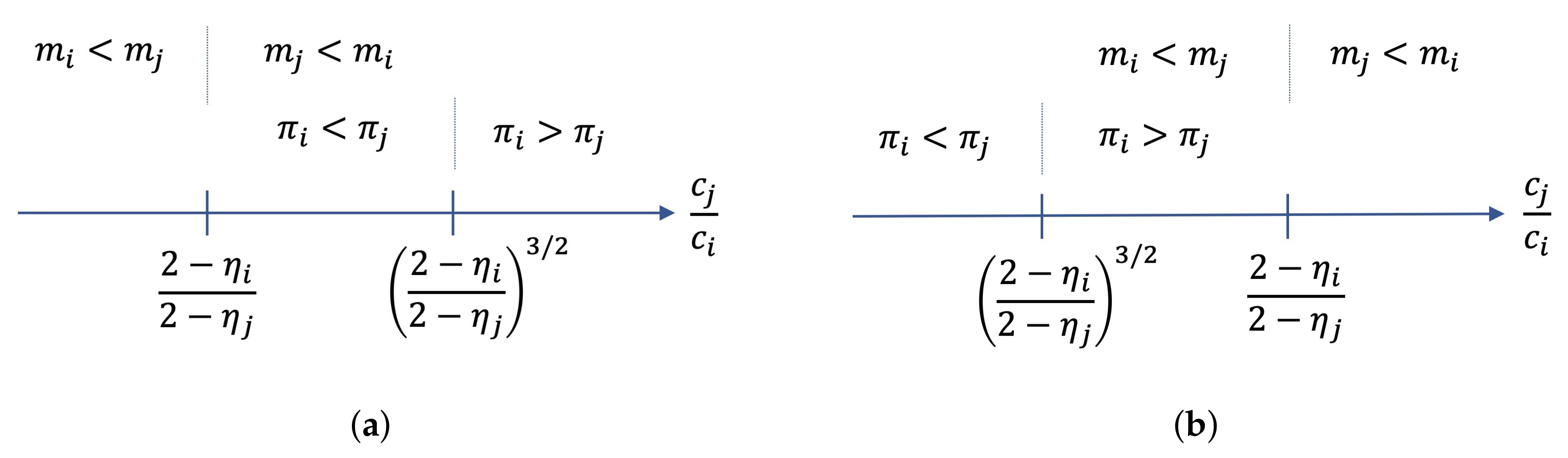
The asset stock of platform i is larger than the asset stock of platform j in period t { 1 , 2 } iff c j c i > 2 η i 2 η j .
(iii) 
Stronger network effects on platform i always increase the asset stock of platform i, while stronger network effects on platform j increase the asset stock of platform i iff c j c i > 2 η i 2 η j .
(iv) 
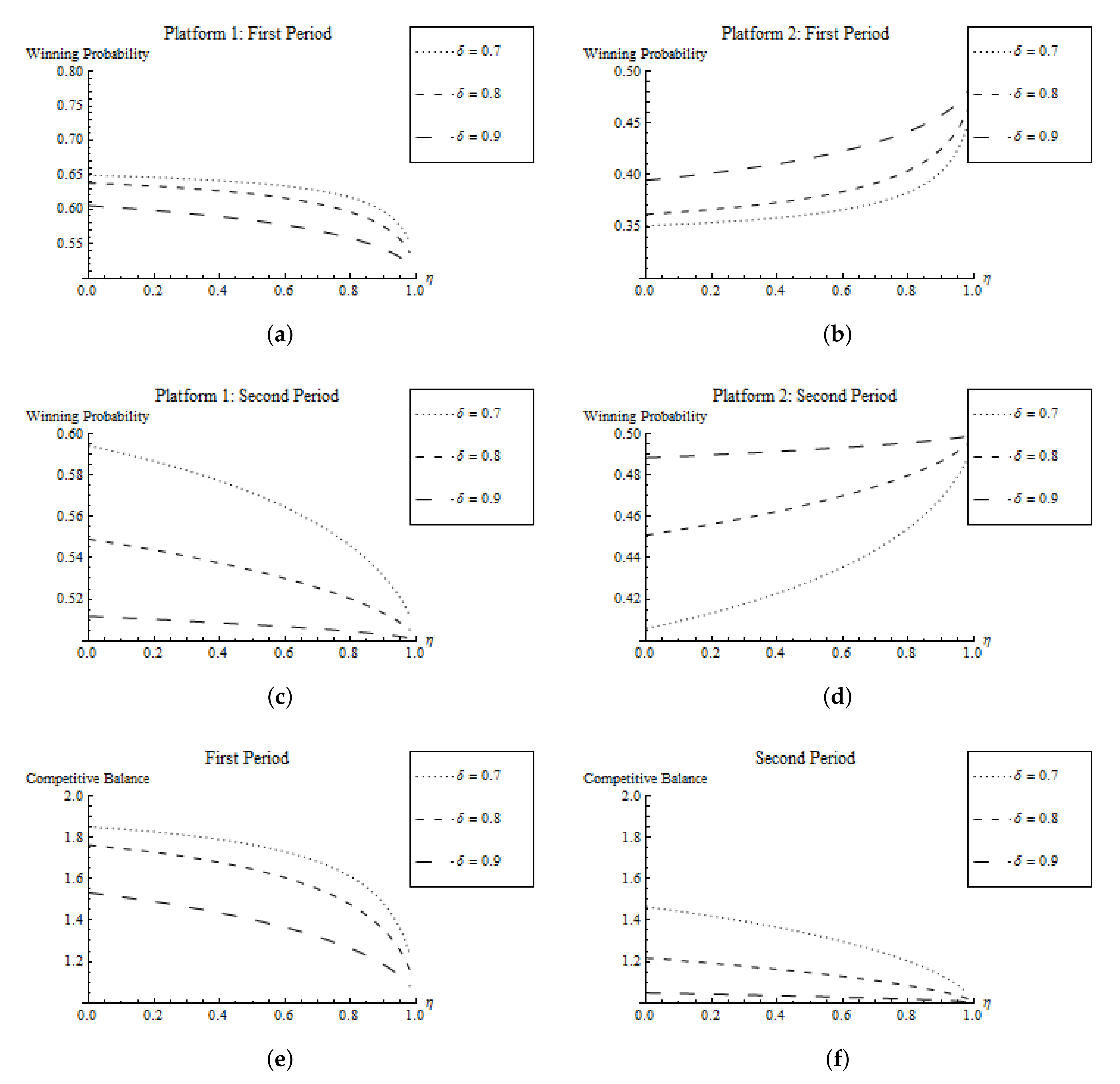
The winning probability of platform i increases with larger network effects on the own platform and it decreases with stronger network effects on the other platform, i.e., w i , t * η i > 0 and w i , t * η j < 0 . Hence, larger network effects η i on platform i increase the balance of the contest if c j c i < 2 η i 2 η j .
Proof. 
The proof is straightforward and therefore omitted. □
Part (i) shows that the asset stock is always higher in Period 1 than in Period 2, i.e., m i , 1 * > m i , 2 * because 1 / 1 β ( 1 δ ) > 1 . That is, a dynamic competition leads to higher investments in asset stock today since part of the asset stock is also valuable in the future. The lower the depreciation rate δ and/or the higher the discount factor β , the larger the incentives to invest in the asset stock today. This result may explain why Apple, as the producer of iPads, makes large investments in R&D. Apple anticipates that today’s investments are also partly valuable in the future, when new versions are released.
Regarding Part (ii), we find that whether platform i has a higher asset stock than platform j in period t { 1 , 2 } depends on the relationship between relative costs and relative network effects. Formally, we derive:
m i , t * > m j , t * c j c i > 2 η i 2 η j .
Note that lower marginal costs and higher network effects increase a platform’s incentive to invest.
In the case of symmetric network effects, i.e., η i = η j , the platform with the lower costs has the higher asset stock in equilibrium in both periods. On the other hand, in case of symmetric costs, i.e., c i = c j , the platform with the stronger combined network effects has the higher asset stock in equilibrium in both periods. Combining both results, we see that stronger network effects can compensate for higher costs. This result suggests that a developer of a tablet PC should not just be interested in cost efficiency to prevail in a market. A competitive advantage may also arise from higher network effects. For instance, Apple’s App Store may increase these network effects by connecting the two sides (app producers and app users) more closely.
Part (iii) shows that asset stocks always increase in own network effects, i.e., m i , t * η i > 0 , while the impact of stronger network effects on the other platform depends on the relationship between relative costs and relative network effects. In particular, asset stocks on the own platform increase in the network effects of the other platform, i.e., m i , t * η j > 0 if the own platform has a higher asset stock in equilibrium, i.e., m i , t * > m j , t * so that condition (8) holds. This result suggests that Apple has incentives to improve their technology (e.g., through higher R&D investments) if the network effects on their platform increase. However, if the network effects on the competing platform increase, Apple will improve their technology only if they are already the dominating platform characterized through a better technology, i.e., a larger asset stock.
According to Part (iv), the probability that a platform wins the platform contest increases in own network effects, and it decreases in the network effects of the other platform. Assume that platform i has a higher level of asset stocks than platform j. It follows that stronger network effects η i on platform i makes the platform contest less balanced and stronger network effects η j on platform j makes the platform contest more balanced. This result suggests that Apple might defend its head start by trying to find ways to increase their network effects. In this case, Apple directly benefits through an increase in its asset stock. In addition, there is an indirect effect on the opponent’s behavior because Apple’s opponents have fewer incentives to improve their technology. As a consequence, the contest becomes less balanced and Apple can further increase its advantage.
Next, we derive the optimal investment path for both platforms in the following proposition.
Proposition 3.
(i) 
In Period 1, the manager of platform i invests the following:
x i , 1 * = m i , 1 * ( 1 δ ) m i , 0 = 1 1 β ( 1 δ ) c j ( 2 η j ) c i ( 2 η i ) + c j ( 2 η j ) 2 ( 1 δ ) m i , 0
to build up asset stock given by m i , 1 * .
(ii) 
In Period 2, the manager of platform i invests the following:
x i , 2 * = m i , 2 * ( 1 δ ) m i , 1 * = δ β ( 1 δ ) 1 β ( 1 δ ) c j ( 2 η j ) c i ( 2 η i ) + c j ( 2 η j ) 2
to build up asset stock given by m i , 2 * .
Proof. 
The proof is straightforward and therefore omitted. □
To see the interplay between costs and initial asset stock m i , 0 , we assume that platform j has a head start in the beginning of the contest in Period 0. Thus, platform j has a higher initial asset stock than platform i, i.e., m j , 0 > m i , 0 . In addition, suppose that condition (8) holds for t = 1 . In this case, we know that platform i will have a higher asset stock in Period 1 than platform j. That is, independently of initial asset stocks, platform i will have a higher probability to win the competition in Period 1. The reason is that platform i will invest more than platform j in Period 1, such that an immediate leapfrogging occurs. Note that the lower the m i , 0 , the higher the first-period investments x i , 1 * of platform i. Thus, initial asset stocks in t = 0 are not decisive regarding future winning probabilities if costs are linear.
The effects of the head start in Period 0 on winning probabilities are immediately wiped out in Period 1. Initial asset stocks only affect the size of the first-period investments. One could argue that, even if Apple had some technological advance with its iPad, it can only sustain this advantage if the cost efficiency in combination with the network effects is superior, compared to the competitor. Samsung has adumbrated with its Galaxy Tab S7 that a catch up or even a leapfrogging can occur quite quickly.
Moreover, in the case that initial asset stocks are zero for both platforms, second-period investments x i , 2 * are always lower than first-period investments x i , 1 * since part of the first-period asset stocks can be used in the second period.
Finally, we derive expected profits of the two platforms and we analyze how costs and network effects influence expected profits.
Proposition 4.
(i) 
Expected profits of platform i { 1 , 2 } in equilibrium are given by the following:
π i * = π i , 1 * + β π i , 2 * = ( 1 + β ) c j 2 ( 2 η j ) 2 ( 2 η i ) c i ( 2 η i ) + c j ( 2 η j ) 2 + c i ( 1 δ ) m i , 0
with i , j { 1 , 2 } and i j .
(ii) 
We derive the following comparative statics:
π i * m i , 0 > 0 , π i * c i > 0 , π i * c j < 0 π i * η i > 0 , π i * η j < 0
Proof. 
The proof is straightforward and therefore omitted. □
The comparative statics analysis shows that higher initial asset stocks m i , 0 yield higher overall platform profits. This result is intuitive because a higher initial asset stock m i , 0 reduces investment costs c i x i , 1 * = c i m i , 1 * c i ( 1 δ ) m i , 0 in Period 1. However, less intuitive and more interesting is the fact that higher marginal costs c i on the own platform produce higher expected profits. On the other hand, higher marginal costs c j on the other platform produce lower expected profits. Finally, we derive that expected profits increase in own network effects and decrease in the network effects of the other platform.
Next, we assume that m i , 0 = 0 for i { 1 , 2 } . We derive the following:
π i * > π j * c j c i > 2 η i 2 η j 3 / 2
with i , j { 1 , 2 } and i j according to result (i). Basically, the same reasoning applies to a platform’s profit as above. Stronger network effects compensate for higher costs. The difference, however, is that the network-related effect is stronger than the cost-related effect. For 1 < 2 η i 2 η j < c j c i < 2 η i 2 η j 3 / 2 , platform i has larger asset stocks but lower expected profits than platform j (see Figure 1a). For 2 η i 2 η j 3 / 2 < c j c i < 2 η i 2 η j < 1 , platform i has larger expected profits but lower asset stocks than platform j (see Figure 1b). Thus, we obtain the following corollary:
Corollary 1.
A dominance in a market characterized by a larger asset stock and therefore by a larger winning probability in the contest does not have to imply a higher (expected) profitability.
Proof. 
The proof is straightforward and therefore omitted. □
Corollary 1 provides a theoretical foundation that a firm’s size and profit are not necessarily positively correlated. Smaller platforms possibly are more profitable than larger platforms.
To sum up, this section has focused on the effect of heterogeneity with respect to costs and network effects. The assumption of linear costs is very helpful to simplify matters with respect to the dynamics. In the case of linear costs, symmetric marginal costs c i = c j and symmetric network effects η i = η j , the winning probabilities and consequently competitive balance are equal in Periods 1 and 2 and do not depend on the depreciation rate δ . Moreover, the dynamics regarding the other variables are trivial because convergence of the asset stocks immediately results in Period 1 (even for different initial asset stocks in Period 0).
However, a comparative advantage of a firm does not necessarily translate immediately into a competitive advantage. The transition from an underdog to a favorite might be driven by other factors, such as rigidities with respect to investments. These rigidities can be introduced into the model by assuming strictly convex costs, which we will model in the next section.

4.3. Quadratic Costs and Homogeneity
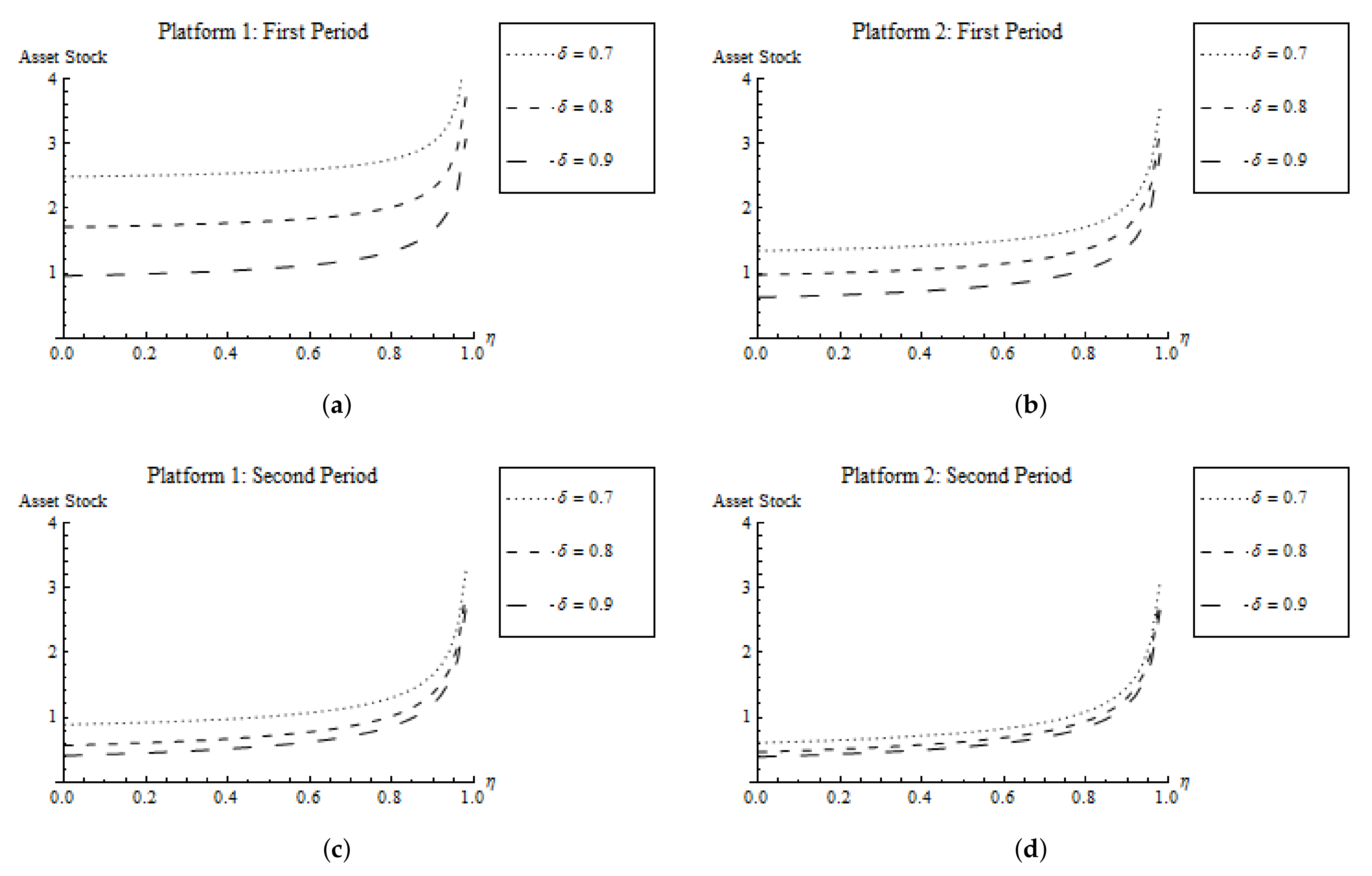
To gain more insights into the dynamics of the contest, we introduce strictly convex costs given by c i ( x i , t ) = ( 1 / 2 ) x i , t 2 . For tractability, we assume that the platforms have symmetric cost functions and that the network effects are the same on both platforms, i.e., η i = η j = η . Thus, the platforms only differ with respect to their initial asset stock. Note that we only analyze the open-loop equilibrium in this section.
We assume that platform 1 is the “large” platform in Period 0 and set m 1 , 0 = 8 and m 2 , 0 = 4 . Moreover, we set β = 1 , γ = 1 and consider specific values for the network effect η = [ 0 , 1 ) and the depreciation rate δ { 0.7 , 0.8 , 0.9 } . We derive the following proposition:
Proposition 5.
(i) 
A lower depreciation rate δ or stronger network effects η increase asset stocks m i , t * for platform i in period t.
(ii) 
A higher depreciation rate δ or stronger network effects η increase the speed of convergence of asset stocks m i , t * for platform i in period t.
Proof. 
We have to rely on numerical simulations because it is analytically not possible to derive the results with quadratic costs in closed form. We run numerous simulations and received always similar results (all simulations are available upon request). □
Result (i) is intuitive because it shows that a low depreciation rate (high technological carry-over) and/or stronger network effects increase incentives to invest into the platforms and thus increase the asset stocks. The result is illustrated in Figure 2. Note that in the case of linear costs, a lower depreciation rate increases the asset stocks only in Period 1. However, the depreciation rate has no effect on the asset stocks in Period 2 for linear costs (see Proposition 1).
Results (ii) examines the speed of convergence: We know from the previous section that in the case of linear costs, the winning probabilities already converge in Period 1, resulting in a fully balanced competition. However, in the case of quadratic costs, convergence of the winning probabilities does not occur, neither in Period 1 nor in Period 2 (compare Figure 3). Platform 1 benefits in both periods from the head start in Period 0, yielding an unbalanced contest with a competitive balance larger than those in Periods 1 and 2.
The simulation further shows that a higher depreciation rate δ and stronger network effects η increase the balance of the contest in period t. This result means that heterogeneity with respect to asset stocks originating from the initial asset stocks are wiped out faster for a larger depreciation rate or stronger network effects. Therefore, we expect, according to our model, that a start-up firm catches up to the "incumbent" faster in an industry characterized by a high deprecation rate (low technological carry-over) and strong network effects. On the other hand, the combination of a low deprecation rate (high technological carry-over) and weak network effects can be responsible for the emergence of a long-lasting dominance of a specific platform.

5. Discussion and Conclusions

Platforms enable two or more market sides to interact with each other. Typical examples are credit cards, video game consoles, internet auctions, smartphones and tablets. Since participants on one side of the platform derive a substantial amount of their utility from the platform participants on the other market side(s), competition among platforms is characterized by network externalities. If these network externalities are important, platform competition will ultimately result in winner-take-all or at least winner-take-most markets. Consequently, such a platform competition takes the form of a dynamic contest for (periodic) market dominance.
To enhance our understanding of such dynamic platform competitions, we have developed a contest model to analyze the competition between two platforms over time. We show that there is a closed-loop and open-loop equilibrium in which both platforms heavily compete for the winner-take-all market. The probability of winning the market depends on the initial competitive position (asset stock) and network effects of each platform. We further show that investment costs and network effects are (negative) substitutes.
Our findings have several implications for research and practice. First, platforms that succeed in attracting a large number of participants on both sides can compensate for cost disadvantages with network effects. Consequently, platform managers shall focus not only on cost efficiency but also on network mobilization (e.g., by connecting the two market sides more closely in order to strengthen the network effects).
Second, the initial competitive position of both platforms is irrelevant for future winning probabilities if costs are linear. The individual probabilities of winning the market only depend on costs and network effects. This result has important strategic implications for platform firms and their managers. Market entrants and late movers should not be distracted by the investments of the first mover because they will be able to leapfrog the incumbent if they succeed in mobilizing their network effects and/or have cost advantages. Therefore, a combined effect of a head start, cost advantages and network effects primarily drives the winning probabilities and profits in equilibrium.
Third, a market dominance does not automatically translate into higher profits. A platform firm can have accumulated more asset stocks (knowledge and technological level of the platform) in the past but can simultaneously be less profitable than a competitor. Our results show that convex costs can explain the long-lasting effects of head starts. Larger relative asset stocks in the beginning can imply larger winning probabilities in the future. However, the advantage is diminished for stronger network effects or lower technological carry-over.
Our study contributes to several related streams of research in economic theory. In particular, our paper combines the theory of multi-sided markets with dynamic contest models to capture important characteristics of platform competition observed in real-world examples (such as Apple vs. Samsung). On the one hand, we extend the contest theory literature by integrating network externalities into a dynamic contest model. On the other hand, we extend the literature on two-sided markets by taking into account that platforms often compete with each other for market shares via a contest. The combination of these two bodies of literature yields fruitful insights that are not captured by, e.g., static contest models. For example, our dynamic contest model with network externalities provides new insights with respect to the underlying causes for the emergence of market dominance of certain platform firms. The combination of technological carry-over and network effects can explain a long-lasting dominance of a platform that benefits from a head start (represented through higher initial asset stocks). The necessary preconditions for the emergence of a long-lasting dominance are convex costs, small network effects and high technological carry-over. On the other hand, we expect that a start-up firm catches up to the "incumbent" faster in an industry characterized by low technological carry-over and strong network effects. If costs are linear, convergence occurs already in Period 1 such that a head start of an incumbent platform is wiped out. In this case, an incumbent can only sustain its advantage if the cost efficiency in combination with the network effects is superior compared to the competitor.
Our model may serve as a basic framework to further analyze dynamic platform competition in two-sided markets. There is a broad range of further applications and model extensions. For instance, an interesting avenue for further research could be the extension of our model to more than two market sides. The implementation of a third market side, such as advertisers, could shed more light on the impact of network externalities. Another promising avenue for further research is the extension of our model in order to conduct a welfare analysis in the framework of a dynamic model of platform competition in two-sided markets. Furthermore, interesting extensions could be to examine other contest success functions, or to abstract from a winner-takes-all market and to study other market environments.
In sum, the issues surrounding the implications of dynamics in platform competition remain a fertile and important line of inquiry for economics, business and management.

Author Contributions

Conceptualization, M.G., M.L. and H.M.D.; methodology, M.G. and M.L.; formal analysis, M.G. and M.L.; writing—original draft preparation, M.G. and M.L.; writing—review and editing, M.G. and M.L.; visualization, M.G. and M.L.; supervision, H.M.D. All authors have read and agreed to the published version of the manuscript.

Funding

This research received no external funding.

Institutional Review Board Statement

Not applicable.

Informed Consent Statement

Not applicable.

Acknowledgments

We would to like to thank three anonymous referees, who significantly helped to improve the paper.

Conflicts of Interest

The authors declare no conflict of interest.

Abbreviations

The following abbreviations are used in this manuscript:
PCPersonal Computer
VHSVideo Home System
OTTOver-The-Top
CSFContest Success Function
CBCompetitive Balance

Appendix A

Appendix A.1. Proof of Lemma 1

We can solve the maximization problem by replacing prices and maximizing π i , 2 with respect to quantities q i , 2 1 and q i , 2 2 :
max q i , 2 a , q i , 2 b π i , 2 = w i , 2 · 1 q i , 2 a + n i b q i , 2 b q i , 2 a + 1 q i , 2 b + n i a q i , 2 a q i , 2 b c i ( x i , 2 )
The first-order conditions are given by the following:
π i , 2 q i , 2 a = w i , 2 1 2 q i , 2 a + n i b q i , 2 b + n i a q i , 2 b = 0
π i , 2 q i , 2 b = w i , 2 1 2 q i , 2 b + n i a q i , 2 a + n i b q i , 2 a = 0
Therefore, it is easy to see that q i , 2 a = q i , 2 b in equilibrium. Using this result in one of first-order condition, we receive the following:
q i , 2 a = q i , 2 b = 1 2 ( n i a + n i b )
Replacing the optimal quantities in the demand functions, we obtain the following:
p i , 2 a = 1 n i a 2 ( n i a + n i b ) p i , 2 b = 1 n i b 2 ( n i a + n i b )
Therefore, we have derived the optimal prices in Period 2 as stated in Lemma 1.

Appendix A.2. Proof of Lemma 4

The first-order condition is given by the following:
γ m i , 1 γ 1 m j , 1 γ m i , 1 γ + m j , 1 γ 2 1 2 ( n i a + n i b ) + β ( 1 δ ) c i ( x i , 2 ) x i , 2 = c i ( m i , 1 ( 1 δ ) m i , 0 ) m i , 1 μ i κ i
with
μ i π i m i , 2 = 0 m i , 2 * ( m j , 1 * , m i , 1 ) m i , 1
and
κ i π i m j , 2 m j , 2 * ( m j , 1 * , m i , 1 ) m i , 1 .
Note that π i / m i , 2 = 0 , due to the envelope theorem. Therefore, the first-order condition reduces to the following:
γ m i , 1 γ 1 m j , 1 γ m i , 1 γ + m j , 1 γ 2 1 2 ( n i a + n i b ) + β ( 1 δ ) c i ( x i , 2 ) x i , 2 = c i ( m i , 1 ( 1 δ ) m i , 0 ) m i , 1 κ i
Dividing the two first-order conditions, we obtain the following:
γ m i , 1 γ 1 m j , 1 γ m i , 1 γ + m j , 1 γ 2 1 2 ( n i a + n i b ) + β ( 1 δ ) c i ( x i , 2 ) x i , 2 γ m j , 1 γ 1 m i , 1 γ m i , 1 γ + m j , 1 γ 2 1 2 ( n j a + n j b ) + β ( 1 δ ) c j ( x j , 2 ) x j , 2 = c i ( m i , 1 * ( 1 δ ) m i , 0 ) m i , 1 κ i c j ( m j , 1 * ( 1 δ ) m j , 0 ) m j , 1 κ j ,
Therefore, we have derived the results stated in Lemma 4.

References

  1. Wright, J. One-Sided Logic in Two-Sided Markets. Rev. Netw. Econ. 2004, 3, 44–64. [Google Scholar] [CrossRef]
  2. Rysman, M. The Economics of Two-Sided Markets. J. Econ. Perspect. 2009, 23, 125–143. [Google Scholar] [CrossRef] [Green Version]
  3. Ihlström Eriksson, C.; Akesson, M.; Lund, J. Designing Ubiquitous Media Services-Exploring the Two-Sided Market of Newspapers. J. Theor. Appl. Electron. Commer. Res. 2016, 11, 1–19. [Google Scholar] [CrossRef] [Green Version]
  4. Landsman, V.; Stremersch, S. Multihoming in Two-Sided Markets: An Empirical Inquiry in the Video Game Console Industry. J. Mark. 2011, 75, 39–54. [Google Scholar] [CrossRef]
  5. Netflix Is Still Growing Wildly, but Its Market Share Has Fallen to an Estimated 19% as New Competitors Emerge. Available online: https://www.businessinsider.com/netflix-market-share-of-global-streaming-subscribers-dropping-ampere-2020-1 (accessed on 1 May 2021).
  6. Staykova, K.; Damsgaard, J. A 2020 Perspective on “the Race to Dominate the Mobile Payments Platform: Entry and Expansion Strategies”. Electron. Commer. Res. Appl. 2020, 41, 100954. [Google Scholar] [CrossRef]
  7. Staykova, K.S.; Damsgaard, J. Adoption of Mobile Payment Platforms: Managing Reach and Range. J. Theor. Appl. Electron. Commer. Res. 2016, 11, 65–84. [Google Scholar] [CrossRef] [Green Version]
  8. Evans, D.; Schmalensee, R. The Antitrust Analysis of Multisided Platform Businesses. In Oxford Handbook on International Antitrust Economics; Blair, R.D., Sokol, D.D., Eds.; Oxford University Press: Oxford, UK, 2014. [Google Scholar]
  9. Pontual Ribeiro, E.; Golovanova, S. A Unified Presentation Of Competition Analysis In Two-Sided Markets. J. Econ. Surv. 2020, 34, 548–571. [Google Scholar] [CrossRef]
  10. Wilbur, K.C. A Two-Sided, Empirical Model of Television Advertising and Viewing Markets. Mark. Sci. 2008, 27, 356–378. [Google Scholar] [CrossRef] [Green Version]
  11. Liu, H. Dynamics of Pricing in the Video Game Console Market: Skimming or Penetration? J. Mark. Res. 2010, 47, 428–443. [Google Scholar] [CrossRef]
  12. Chu, J.; Manchanda, P. Quantifying Cross and Direct Network Effects in Online Consumer-to-Consumer Platforms. Mark. Sci. 2016, 35, 870–893. [Google Scholar] [CrossRef]
  13. Hinz, O.; Otter, T.; Skiera, B. Estimating Network Effects in Two-Sided Markets. J. Manag. Inform. Syst. 2020, 37, 12–38. [Google Scholar] [CrossRef]
  14. Rochet, J.C.; Tirole, J. Two-Sided Markets: A Progress Report. RAND J. Econ. 2006, 37, 645–667. [Google Scholar] [CrossRef] [Green Version]
  15. Weyl, E.G. A Price Theory of Multi-Sided Platforms. Am. Econ. Rev. 2010, 100, 1642–1672. [Google Scholar] [CrossRef]
  16. Roger, G.; Vasconcelos, L. Platform Pricing Structure and Moral Hazard. J. Econ. Manag. Strategy 2014, 23, 527–547. [Google Scholar] [CrossRef] [Green Version]
  17. Ribeiro, V.M.; Bao, L. Professionalization of Online Gaming? Theoretical and Empirical Analysis for a Monopoly-Holding Platform. J. Theor. Appl. Electron. Commer. Res. 2021, 16, 682–708. [Google Scholar] [CrossRef]
  18. Caillaud, B.; Jullien, B. Competing Cybermediaries. Eur. Econ. Rev. 2001, 45, 797–808. [Google Scholar] [CrossRef] [Green Version]
  19. Jullien, B. Competition in multi-sided markets: Divide and conquer. Am. Econ. J. Macroecon. 2011, 3, 186–220. [Google Scholar] [CrossRef]
  20. Hossain, T.; Morgan, J. When Do Markets Tip? A Cognitive Hierarchy Approach. Mark. Sci. 2013, 32, 431–453. [Google Scholar] [CrossRef] [Green Version]
  21. Caillaud, B.; Jullien, B. Chicken & Egg: Competition among Intermediation Service Providers. RAND J. Econ. 2003, 34, 309–328. [Google Scholar]
  22. Rochet, J.C.; Tirole, J. Platform Competition in Two-Sided Markets. J. Eur. Econ. Assoc. 2003, 1, 990–1029. [Google Scholar] [CrossRef] [Green Version]
  23. Armstrong, M. Competition in Two-Sided Markets. RAND J. Econ. 2006, 37, 668–691. [Google Scholar] [CrossRef] [Green Version]
  24. Liu, Q.; Serfes, K. Price Discrimination in Two-Sided Markets. J. Econ. Manag. Strategy 2013, 22, 768–786. [Google Scholar] [CrossRef]
  25. Lee, R.S. Competing Platforms. J. Econ. Manag. Strategy 2014, 23, 507–526. [Google Scholar] [CrossRef]
  26. Hałaburda, H.; Yehezkel, Y. The Role of Coordination Bias in Platform Competition. J. Econ. Manag. Strategy 2016, 25, 274–312. [Google Scholar] [CrossRef] [Green Version]
  27. Liu, Q. Stability and Bayesian Consistency in Two-Sided Markets. Am. Econ. Rev. 2020, 110, 2625–2666. [Google Scholar] [CrossRef]
  28. Konrad, K.A. Strategy and Dynamics in Contests; Oxford University Press: Oxford, UK, 2009. [Google Scholar]
  29. Clark, D.J.; Nilssen, T. Learning by Doing in Contests. Public Choice 2013, 156, 329–343. [Google Scholar] [CrossRef]
  30. Grossmann, M.; Lang, M.; Dietl, H.M. Transitional Dynamics in a Tullock Contest with a General Cost Function. BE J. Theor. Econ. 2011, 11. [Google Scholar] [CrossRef] [Green Version]
  31. Grossmann, M.; Dietl, H.M. Investment Behaviour in a Two-Period Contest Model. J. Inst. Theor. Econ. 2009, 165, 401–417. [Google Scholar] [CrossRef]
  32. Yildirim, H. Contests with Multiple Rounds. Games Econ. Behav. 2005, 51, 213–227. [Google Scholar] [CrossRef] [Green Version]
  33. Baik, K.H.; Lee, S. Two-Stage Rent-Seeking Contests with Carryovers. Public Choice 2000, 103, 285–296. [Google Scholar] [CrossRef]
  34. Lee, S. Two-Stage Contests with Additive Carryovers. Int. Econ. J. 2003, 17, 83–99. [Google Scholar] [CrossRef]
  35. Keskin, K.; Saglam, C. Investment on Human Capital in a Dynamic Contest Model. Stud. Nonlinear Dyn. Econom. 2019, 23, 20170095. [Google Scholar] [CrossRef] [Green Version]
  36. Matsumoto, A.; Szidarovszky, F. Dynamic Contest Games with Time Delays. Int. Game Theory Rev. 2020, 22, 1950017. [Google Scholar] [CrossRef]
  37. Zhang, M.; Wang, G.; Xu, J.; Qu, C. Dynamic Contest Model with Bounded Rationality. Appl. Math. Comput. 2020, 370, 124909. [Google Scholar] [CrossRef]
  38. Tullock, G. Efficient Rent Seeking. In Efficient Rent-Seeking: Chronicle of an Intellectual Quagmire; Lockard, A.A., Tullock, G., Eds.; Springer US: Boston, MA, USA, 1980; pp. 3–16. [Google Scholar]
  39. Skaperdas, S. Contest Success Functions. Econ. Theory 1996, 7, 283–290. [Google Scholar] [CrossRef]
  40. Clark, D.J.; Riis, C. Contest Success Functions: An Extension. Econ. Theory 1998, 11, 201–204. [Google Scholar] [CrossRef]
  41. Lazear, E.P.; Rosen, S. Rank-Order Tournaments as Optimum Labor Contracts. J. Pol. Econ. 1981, 89, 841–864. [Google Scholar] [CrossRef] [Green Version]
  42. Dixit, A. Strategic Behavior in Contests. Am. Econ. Rev. 1987, 77, 891–898. [Google Scholar]
  43. Hirshleifer, J. Conflict and Rent-Seeking Success Functions: Ratio Vs. Difference Models of Relative Success. Public Choice 1989, 63, 101–112. [Google Scholar] [CrossRef]
  44. Runkel, M. Total Effort, Competitive Balance and the Optimal Contest Success Function. Eur. J. Political Econ. 2006, 22, 1009–1013. [Google Scholar] [CrossRef]
  45. Fudenberg, D.; Tirole, J. Game Theory; The MIT Press: Cambridge, MA, USA, 1991. [Google Scholar]
Figure 1. Asset stocks and profits for linear costs. (a) Case 2 η i > 2 η j , (b) Case 2 η i < 2 η j .
Jtaer 16 00117 g001
Figure 2. Asset stocks for quadratic costs. (a) Platform 1: First period, (b) Platform 2: First period, (c) Platform 1: Second period, (d) Platform 2: Second period.
Jtaer 16 00117 g002
Figure 3. Winning probabilities and competitive balance for quadratic costs. (a) Platform 1: First period, (b) Platform 2: First period, (c) Platform 1: Second period, (d) Platform 2: Second period, (e) First period, (f) Second period.
Jtaer 16 00117 g003
Publisher’s Note: MDPI stays neutral with regard to jurisdictional claims in published maps and institutional affiliations.

