
Multi-Layer Fuzzy Sustainable Decision Approach for Outsourcing Manufacturer Selection in Apparel and Textile Supply Chain


Department of Industrial Engineering and Management, National Kaohsiung University of Science and Technology, Kaohsiung 80778, Taiwan
*
Authors to whom correspondence should be addressed.
Axioms 2021, 10(4), 262; https://doi.org/10.3390/axioms10040262
Submission received: 14 September 2021
/
Revised: 4 October 2021
/
Accepted: 6 October 2021
/
Published: 19 October 2021
(This article belongs to the Special Issue Decision Analysis with Optimization Technique)
Abstract
:The apparel and textile industry are known as a key sector in the structure of many economies around the world. In particular, the influence of foreign outsourcing manufacturers on textile supply chains has been recognized for decades. The outsourcing manufacturers are multi-criteria selected and changed by supply chain managers from time to time in search of the most efficient state for the entire supply chain. This is a known concern with the community and there is large interest in studying the apparel and textile outsourcing manufacturer problems. Aiming at reinforcing the selection methods, this study develops a three-layer fuzzy multiple criteria decision-making approach that leverages the strengths from the original methods. In turn through the layers, the hierarchy and weights of criteria and sub-criteria, which includes sustainability factors, are determined by the fuzzy analytic hierarchy process (FAHP) method. Next, the results from the fuzzy technique for order of preference by similarity to ideal solution (FTOPSIS) process determine the outsourcing manufacturer’s performance via expert linguistics judgments. Then, data envelopment analysis (DEA) models are applied for the purpose of evaluating the outsourcing manufacturer’s overall performance along with other quantitative effectiveness. This approach is applied to the problem of selecting the apparel and textile outsourcing manufacturers in Vietnam, one of the places that makes the necessity of this problem grow. The third position in the world apparel and textile export ranking, as well as the trend of shifting labor-intensive production systems to Southeast Asia make the necessity of Vietnam outsourcing manufacturer selection problem grow. The results of this study also classified manufacturers into groups as a support for selection decisions. Analysis of quantitative uncertainties using simulation tools and forecasting techniques can strengthen the solutions in future related studies.
1. Introduction
During the COVID-19 pandemic, there are still positive signals in the apparel and textile (A&T) industry with an expected increase in demand of over 10% from 2020 to 2021, according to the World Bank’s global market report [1]. As a result, A&T supply chains are believed to remain viable and contribute significantly to economies around the world. In which, A&T outsourcing manufacturers (A&TOMs) are the key link to optimize the efficiency of these chains. The efficiency that manufacturers offer is measured in terms of economic benefits and capacity flexibility [2]. The advantages of low labor costs in developing countries have always been considered an important strength of foreign A&TOMs. In addition to economic advantages, there are a few other metrics to evaluate the effectiveness of A&TOMs, such as quality control, services, delivery processes, etc. Foreign A&TOMs with low production costs, tariff advantages but limited logistics services or quality commitments will cause risks of clogging the supply chain. Yet, the impact on the environment also needs to be considered in this regard as a requirement of sustainable development. Therefore, choosing the right A&TOMs has a major influence on the viable performance of multinational supply chains. Research on those metrics has a long tradition. A number of studies and reviews have been undertaken to explore the criteria for the A&TOMs selection problem [3]. These criteria include qualitative or quantitative, numerical or linguistics, stochastic or deterministic categories. Several multiple criteria decisions making (MCDM) methods have been successfully utilized for this purpose. The oldest and most well established are the analytic hierarchy process (AHP), the technique for order of preference by similarity to ideal solution (TOPSIS), and the analytic network process (ANP) [4,5,6]. These methods have been used extensively for solving the problem as weighting and alternative evaluation methods. For efficiency analyses, the data envelopment analysis (DEA) is a mature technology of popular choice [7,8]. In addition, the meta-review presented by Daraio et al. identified gaps and overlaps in empirical surveys in more than twenty areas [9]. In addition, fuzzy logic theory is often used for the purpose of strengthening the above methods when applied under uncertain conditions [10,11,12]. However, no single approach or methodology appears to be universally suitable for both quantitative and qualitive criteria A&TOMs selection problem under uncertainty environment. This motivates the need for an alternative approach where the mentioned methods’ strengths are utilized in a chained manner as three-layer. At the first layer, the fuzzy analytic hierarchy process (FAHP) method is used to determine the selection criteria and sub-criteria, as well as their weights. Then, the expert-based linguistic performance of A&TOMs was calculated using the fuzzy technique for order of preference by similarity to ideal solution (FTOPSIS) process. After defuzzied the results obtained at layer two, the overall performance is analyzed by DEA models along with other objective arithmetic inputs and outputs, such as cost of goods sold, total assets, and gross profit. Finally, A&TOMs are categorized into different groups based on the results of DEA models to aid in selection decisions. This three-layer decision support framework is our original contribution.
As the second contribution, the results of this research have been embodied in a practical application. In the A&T outsourcing industry, Vietnam is currently ranked third in the world after China and Bangladesh. In addition, other studies also show that Vietnam is one of the top destinations for A&T production systems that have shifted from China [13]. Therefore, decisions to select A&TOMs for supply chains are believed to emerge drastically in Vietnam. The three-layer framework proposed in this study has been applied to the problem of selecting A&TOMs in Vietnam to provide a valuable reference for global A&T supply chain managers.
2. Literature Review
This section outlines the existing selection criteria and methods available in literature for A&TOMs selection problem. In the last decade, various studies have determined the criteria and sub-criteria for this problem as shown in Table 1. Criteria related to cost and quality almost always appear in studies as a mandatory requirement for the selection of A&TOMs. In addition, the research also considers the production services, logistics activities, business management, environmentally friendly production systems and technology of A&TOMs as the main selection criteria. Sub-criteria that are related to costs are often referred to by scholars as cost categories and payment convenience. Although International Organization for Standardization (ISO) certifications, quality control statistical performance, and problem-solving support solutions are quality-related sub-criteria. As for the main criterion related to logistics activities, studies show that the sub-criteria mainly revolve around the ability to deliver goods accurately, in both quantity and time. Efficiency and quality of service activities, such as customer service, professionalism, production flexibility is considered as sub-criteria related to production and sales services. In addition, to assess the environmental impact of production systems, sub-criteria on emissions, certificates of environmental standards and environmentally friendly materials are introduced in the studies.
As summarized in Table 2, several methods for alternative selection problems have been reported in the literature, almost the techniques in the literature are from the MCDM field, such as FAHP [5,14,15,18,27,28,29,30,31,32,33,34,35,36,37,38,39,40], FANP [6,27,37,41], FTOPSIS [4,11,29,36,40,42,43], and others [6,18,24,35,43,44]. This problem may have been partly addressed by previous studies by DEA models [5,27,32,33,35,37] and mathematical optimization models [24,45]. These methods are mainly combined by the authors or applied at the same time to compare results. For example, Rashidi compared the results when applying two fuzzy TOPSIS and DEA methods when making supplier selection decisions to rank and evaluate these suppliers from sustainability criteria. The authors want to compare and select the best suppliers from any deviation from the predefined standards in the suppliers from the results of the evaluation [10]. To solving the difficult problem of material selection, Mousavi-Nasab used the MCDM model to provide an extensive assessment. The authors uses two very effective MCDM methods, TOPSIS and the complex proportional assessment (COPRAS), to rank materials due to their reasonable correlation and superior features compared to other studies. On the other hand, DEA can be used on the basis of the known rule of thumb as an aid to solving the material selection problem [43]. In the process industry, Esmaeil Zarei develops a fuzzy coupled multi-criteria decision model to quantify and the resilience was evaluated using the fuzzy analytical hierarchical process and the fuzzy multi-criteria optimization and compromise solution technique (FVIKOR). The weights of the resilience indicators were determined by the FAHP method, while the resilience performance of different operational units was ranked via F-VIKOR method [46]. Wang et al. used the MCDM model combined with simple additive weighting (SAW), TOPSIS, and gray relation analysis (GRA). Ratings that are unified by multiple MCDM methods are more consistent than ratings that are produced by a single MCDM method. The proposed method is demonstrated in a practical utility technique with the participation of an integrated circuit packaging company [47]. To evaluate green suppliers, Gizem ifi and Glin Bykzkan proposed a recent combined analysis approach based on the FTOPSIS, FANP, and fuzzy decision making trial and evaluation laboratory (FDEMATEL) techniques to support strategic decisions. Furthermore, the FTOPSIS method has effectively selected an alternative to the ideal solution of this problem [48].
From different methodologies used in previous studies, it can be seen that AHP, TOPSIS, and DEA methods are the three most prominent and used in different research fields due to their versatility form of their application. AHP is one of the effective mathematical weighting methods to determine the rank of dissimilar attributes with respect to the target. TOPSIS method is one of the widely used MCDM methods in research. To strengthen the solutions by combining the advantages of the above three methods with fuzzy theory, this study proposes a three-layer approach structured with FAHP, FTOPSIS, and DEA models for the A&TOM selection problems.
3. Methodology
3.1. Methodology Description
This study evaluated and selected A&TOMs in Vietnam, in addition to the criteria of qualitive and quantitative criteria. This assessment is based on both subjective linguistic judgment of the experts and objective arithmetic performance. As shown in Figure 1, the study proposed a multi-layer decision making approach for A&TOMs efficiency assessment. In layer 1, the FAHP is used to solve the complex problems of early-stage decision-making. There are four main criteria and twelve sub-criteria are considered for A&TOMs as follows: financial resources (Investment capital and economic ability, raw material prices, freight costs), the quality (ISO standards geographical, technical support, reaction on problem), service (on time delivery, production capacity, customer service), technology criteria (production technology, environmentally friendly systems, improvement efforts). The FTOPSIS is used for rating all alternatives in the layer 2. Through the first and second layers, the expert-based performance (EP) of the A&TOMs were determined. However, these scores also include the opinions and subjective linguistics assessments of experts. To strengthen the solution, DEA models are used to measure the efficiency of DMUs through objective arithmetic performance. In layer 3, DEA models such as the Charnes, Cooper, and Rhodes (CCR) model [52], Banker, Charnes, and Cooper (BCC) model [53], slacks-based measure (SBM) [54], and super SBM [55] in constraint returns-to-scale environment are applied for rating and potential suppliers.
3.2. Fuzzy Set Theory
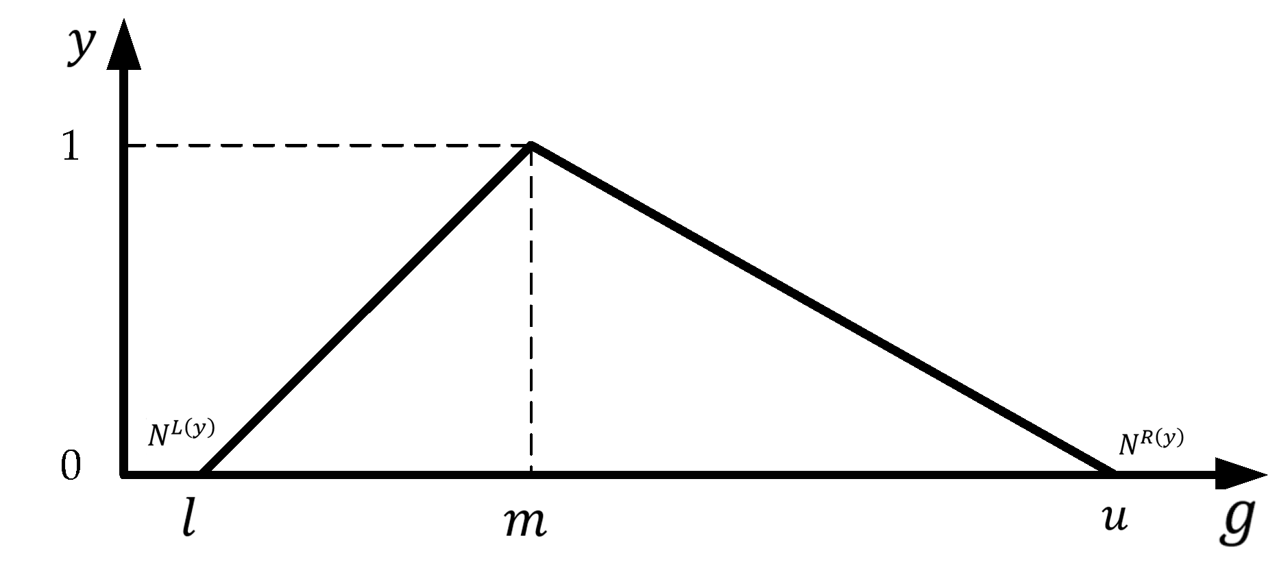
To handle the uncertainty, the triangular fuzzy number (TFN) is defined as representing the most pessimistic, possible and optimistic value, as indicated in Equation (1) and is shown in Figure 2.
As shown in Equation (2), the triangular fuzzy number is given as:
where denotes two side of the TFN.
3.3. Fuzzy Analytical Hierarchy Process (FAHP)
As an uncertainty extension of AHP method, the FAHP method uses quantified pair comparisons with a priority scale of one-nine to establish priorities for each level of the hierarchy as Table 3. In addition to that, FAHP also allows hierarchies and complex relationships between their elements with six-step procedure below.
Step 1: As shown in Equation (3), the fuzzy pairwise comparison matrix is constructed with criteria. In which, presents the importance degree of the criterion th over the th criterion in the th decision maker judgment.
Step 2: The aggregated fuzzy pairwise comparison matrix is calculated as Equation (4). In which, K is the number of decision makers or experts.
Step 3: As shown in Equation (5), the method calculates the fuzzy geometric mean value of each criterion (.
Step4. Calculating the fuzzy weight of each criterion () as Equation (6)
Step 5: As shown in Equation (7), the average value () is used to defuzzify the fuzzy weight of each criterion.
Step 6: Calculating the normalized weight of each criterion () as Equation (8)
In short, the criteria and sub-criteria were determined based on relevant research and survey of experts in the field of A&T in Vietnam. The FAHP procedure calculates the normalize weights of the criteria based on linguistic pairwise comparisons of experts.
3.4. Fuzzy Technique for Order of Preference by Similarity to Ideal Solution (FTOPSIS)
The principle of FTOPSIS is to determine the overall score of alternatives based on the distance to the fuzzy negative ideal solution (FNIS) and the fuzzy positive ideal solution (FPIS). Table 4 describes the linguistic evaluation levels and the corresponding TFN values. The seven steps of the FTOPSIS process are described below.
Step 1: Determine the fuzzy weight of the criteria. These fuzzy weights are the result of calculations in the first layer—FAHP.
Step 2: As seen in Equation (9), the fuzzy decision matrix, which presents the TFN score () of alternatives corresponding to criteria, is constructed based on linguistic evaluation of K experts. The denotation presents for the TFN score of the th alternative with respect to th criterion by th expert’s evaluation. As mentioned in Equation (1), .
Step 3: The normalized fuzzy decision matrix is constructed as Equations (10)–(12).
Step 4: As shown in Equations (13) and (14), this step develops weighted normalized fuzzy decision matrix . The weighted normalized fuzzy score ) is calculated as the product of the normalized fuzzy score () and criteria fuzzy weight ().
Step 5: The fuzzy negative ideal solution () and the fuzzy positive ideal solution are calculated as Equations (14) and (15).
Step 6: This step estimate the distance of each alternative from FNIS and FPIS as Equations (16) and (17).
Step 7: Based on the distances and , the relative gaps-degree of each alternative ) is estimated as Equation (18). The better alternative is the alternative that is farther away than FNIS and closer to FPIS. Therefore, the higher the relative gaps-degree, the higher the alternative is rated by experts.
3.5. Data Envelopment Analysis
3.5.1. Inputs and Outputs Selection
The principal objective of DEA models is to measure the efficiency of using multiple inputs and outputs. From the diverse blend of factors utilized in earlier studies as shown in Table 5, this study selected cost of goods sold (CGS), total assets (TA) as an inputs factor, while gross profit (GP) and expert-based performance (EP) are the outputs.
The correlation between input and output should be isotropic, which implies that the number of inputs and the number of outputs will increase or decrease together under the similar conditions, as shown in Table 6.
The Pearson correlation coefficient ( of two factors and can be calculated as Equation (19), where, and represent the values of the th observation while and presents the mean value of the factors.
3.5.2. DEA Models
Based on ideas from the production efficiency model by Farrell, the first DEA model proposed by Charnes, Cooper, and Rhodes (CCR) [52]. This model determines the efficiency of decision-making units (DMUs) through maximizing the ratio of weighted outputs to weighted inputs. Assume the efficiency of DMUs is measured based on inputs and outputs. The relative efficiency () of each DMU is determined by solving the non-linear model as described in Equations (20)–(23).
subjected to
where denotes the th input and denotes th output of th DMU. Let and denote the virtual variables of th input and th output, respectively.
In addition, the slack () and surplus () variables of the CCR model can suggest directions for improvement as well as input and output values that can optimize efficiency. These variables can be determined by Equations (24) and (25).
where , , , denotes optimal value of and . Accordingly, the th DMU reaches its optimal efficiency when , and .
In 1984, a new model was developed by Banker, Charnes, and Cooper (BCC) based on the CCR model [53]. The BCC model allows a variable return-to-scale (RTS) instead of the constant return-to-scale in the CCR model. The BCC model is presented in the following Equations (26)–(29).
subjected to
where denotes the intercept of production frontier. The positive and negative value of represent the DMU’s production frontier is decreasing RTS and increasing RTS, respectively.
Another DEA model is proposed by Tone in 2001 [54]. This model measures DMU’s efficiency through using input and output slack measurement named lack-based measurement (SBM). In constant RTS environment, the input-oriented SBM (SBM-I-C) can be written as Equations (30)–(33).
subjected to
where denotes input-oriented efficiency value and denotes the weight coefficient of th DMU. Meanwhile, the output-oriented SBM (SBM-O-C) are presented as Equations (34)–(37). In which, the ratio presents the output-oriented efficiency value.
subjected to
In the non-oriented SBM model as Equations (38)–(41), the 0th DMU () is defined as being SBM-efficient if and .
subjected to
In case the objective function’s denominator is equal to one, the model becomes input-oriented super-SBM model. Then, the value of the objective function cannot be less than one.
4. Numerical Results
4.1. Case Study Description
The reality of shifting the outsourcing production system that requires a large labor force among developing countries is increasingly happening [60,61]. In particular, Vietnam is considered as one of the most potential places in Southeast Asia, as well as East Asia [62]. Thanks to that, fashion brands are paying more and more attention to Vietnamese A&TOMs, which have advantages in terms of labor costs and quality. Therefore, choosing an outsourcing garment company that effectively meets multi-criteria becomes the core problem of fashion enterprises at home and abroad in Vietnam.
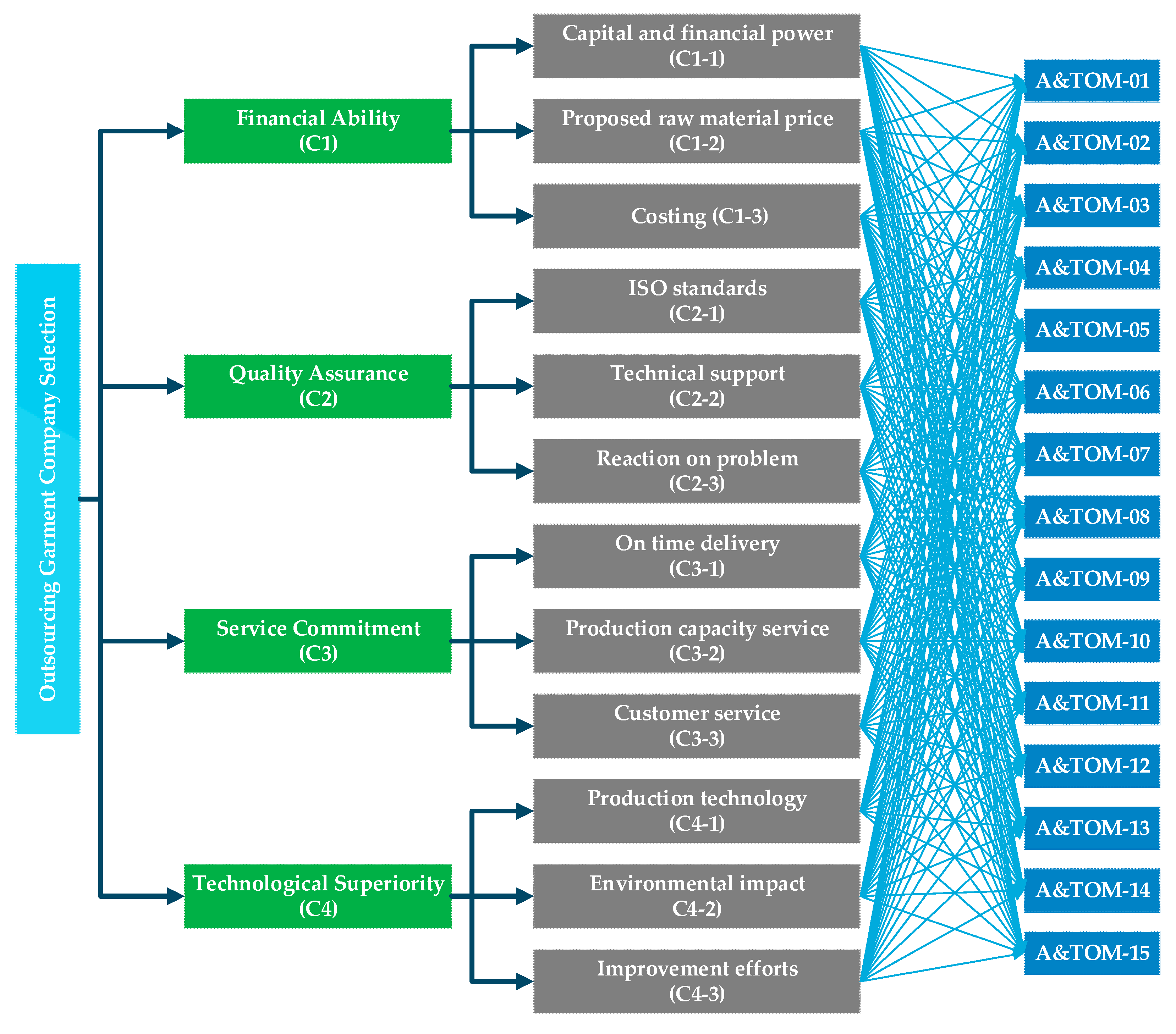
In this study, the proposed fuzzy MCDM model supports to analyze the effectiveness of A&TOMs. Accordingly, the top fifteen A&TOMs in terms of market value were selected for this numerical analysis. Based on literature reviews along with expert survey results, the hierarchy of criteria and sub-criteria for the analysis is depicted in Figure 3. In particular, the criteria showing the capabilities of A&TOMs include financial ability, quality assurance, service commitment, and technological superiority. Twenty experts, with over ten years of experience, consulted and effectively assessed the impact of the criteria and scored the A&TOMs on each sub-criterion in the linguistics levels as Table 4. These professionals are heads of relevant departments from various segments of the garment supply chain.
4.2. Fuzzy AHP Calculation Results
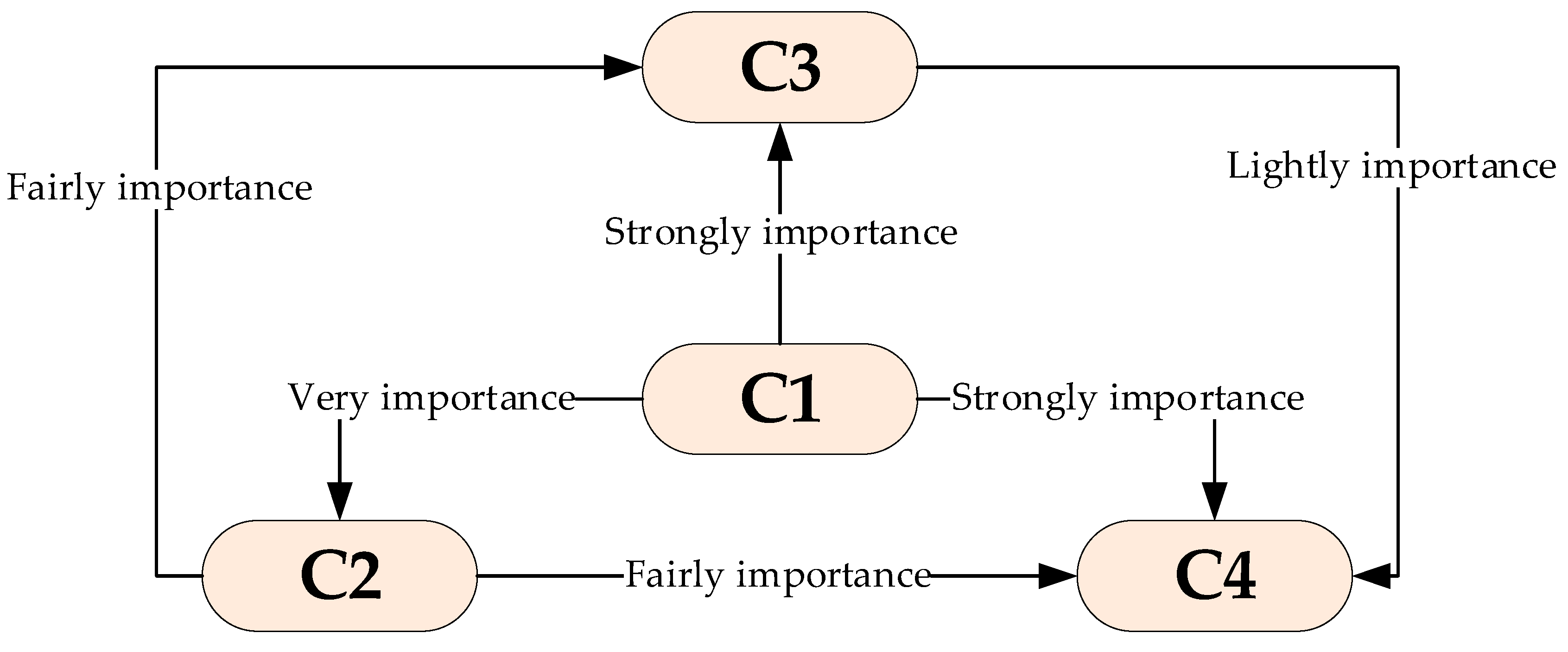
This methodology begins with the weighting of the criteria and sub-criteria through the FAHP calculation procedure. As shown in Figure 4. Criteria linguistics comparison, the results of the criteria linguistics comparison from the expert survey in the first step. Then, the pairwise comparison matrix of the main criteria is surveyed and aggregated as in Table 7.
In order to validate the consistency of this pairwise comparison matrix, fuzzy numbers are defuzzied based on its pessimistic and optimistic values. The non-fuzzy comparison matrix is developed and presented in Table 8.
In Table 9, the non-fuzzy score values are normalized by scaling them to the sum of each column. Then, the priority vector of the criteria are determined as the average value of each row.
As the next step of the consistency determination procedure, the largest eigenvector, which is denoted as is , is estimated as follows.
Because the matrix under consideration is 4 × 4 in size, the value of in the formula that defines is 4.
The consistency index, , and consistency ratio, , are also determined as follows, with the given random index, [63].
The above results show that the coefficient of consistency is less than 10%, so it can be assumed that the consistency of the pairwise comparison matrix is acceptable and can be used for further calculations. This consistency determination procedure is performed similarly for other pairwise comparison matrices. To determine the fuzzy weights of the criteria, the next step is to compute their fuzzy geometric mean, as shown in Table 10.
Then, the study determines the sum of the geometric mean values. Based on the ratio of the geometric mean and the inverse of the sum, the fuzzy weights of the criteria are determined and presented in Table 11.
This weighting procedure is repeated for the pairwise comparison matrices of the sub-criteria. The results of these fuzzy weights are presented in Table 12.
In order to determine the final fuzzy weight of the sub-criteria, the next step is to determine the product of the fuzzy weight of the related sub-criteria and the main criterion as Table 13.
Thus, the weight of the criteria has been determined and this result is also the input parameters of this approach’s layer 2, fuzzy TOPSIS.
4.3. Fuzzy TOPSIS Calculation Results
Following the procedure of FTOPSIS presented in Section 3.4, the fuzzy scores of the alternatives (Table A1 and Table A2, Appendix A) in the decision matrix are normalized (Table A3 and Table A4, Appendix A) and multiplied by the weights in the FAHP result. Then, the normalized weighted scores are defuzzied into real scores (Table A5, Appendix A).
4.4. DEA Calculation Results
The Figure 5 shows inputs and outputs for DMU efficiency analysis by DEA models. The results of the FTOPSIS calculation proposed the expert-based performance (EP) of A&TOMs which are used as an output in DEA models.
According to the definition of efficiency in Section 3.5, indicators are chosen as inputs of the DEA model when its decrease causes the efficiency of a DMU to increase. Additionally, conversely, performance metrics are considered outputs when their increase causes the efficiency of a DMU to increase. The data are collected on the Vietnam stock market, as shown in Table 16.
The variance premise is applied to the input and output variables of the correlation coefficient matrix. Similarly, increasing or decreasing one input does not increase or decrease the other input. The following Table 17 shows the Pearson correlation coefficient testing results.
The results that all coefficients are positive from the results of the Pearson correlation test. It implies that the inputs and output meet the minimal requirement of DEA model under constant returns-of-scale environment.
The data have been collected from fifteen A&TOMs in Vietnam to be able to obtain accurate results in the study. In addition, the hierarchical structure is used to present four main criteria and twelve sub-criteria. We analyze the FTOPSIS model by completing a questionnaire when interviewing experts in the Vietnam A&T industry, in addition to surveying and taking databases from businesses. Then, several DEA models are proposed to rank apparel companies. As a result, A&TOM-10 was determined to be the most efficient of all nine models, as shown in Table 18. Next comes the A&TOM-13 and A&TOM-15 with maximum efficiency in all CCR, BCC, and SBM models. The A&TOM-01, A&TOM-03, A&TOM-08, A&TOM-014 ranked first in either CCR models or BBC models. At the same time, these A&TOMs also rank high in the SBM and super-SBM models. The remaining DMUs are identified as non-efficiency DMUs by the models. Based on the ranking results from the DEA models, this study classifies the A&TOMs into three groups as shown in Figure 6.
5. Conclusions
Over the past three decades, there has been a sustained research activity in apparel and textile supply chain management. One of the cross-cutting concerns of scholars is the issue of selecting outsourcing manufacturers for these supply chains. These selection decisions are influenced simultaneously by multiple criteria and conditions of uncertainty. Combinations of MCDM methods have been introduced and applied by related studies. In order to inherit and consolidate the published combinations of approaches, the main contribution of this study is the proposal of a three-layer approach that effectively vertically combines the three primitive methods. After consulting and defining the four main criteria and twelve sub-criteria for the problem, a hierarchy and pairwise comparison matrices are built. The FAHP procedures are then applied to determine the weighting of the criteria. At the second layer, the expert-based performance of A&TOMs is determined by FTOPSIS decision matrices and procedures. At the last layer, the results of the FTOPSIS method are combined with other objective arithmetic performance to analyze the efficiency of A&TOMs through DEA models. The efficiency rankings from DEA models are now used as a reference for the classification A&TOMs. Second but not least, the proposed three-layer approach is applied to a place that is a promising attraction for outsourcing manufacturer selection decisions, Vietnam. Political stability, low labor costs, preferential tariffs are just a few of the many reasons for Vietnam’s top ranking in the world in processing and exporting the A&T industry. The study proposes criteria and sub-criteria for evaluating A&TOMs from the perspective of this industry experts. In addition, A&TOMs in Vietnam are also classified into three groups as shown in Figure 6. Based on those results, supply chain managers or fashion brand leaders have an additional source of support for their A&TOMs selection decisions in Vietnam. The limitation of this study is that the statistical tests are incomplete on the assumptions of the DEA models, such as convexity, free disposability, and additivity.
For future studies, heuristics algorithms can be integrated to increase the number of A&TOMs that are considered. Simultaneously, simulation and forecasting techniques can support solutions through the development and analysis of uncertainty scenarios.
Author Contributions
Conceptualization, N.-L.N.; methodology, C.-N.W. and N.-L.N.; formal analysis, N.-L.N.; investigation, N.-L.N. and T.-D.T.P.; data curation, T.-D.T.P.; writing—original draft preparation, N.-L.N. and T.-D.T.P.; writing—review and editing, C.-N.W., N.-L.N. and T.-D.T.P.; project administration, C.-N.W.; funding acquisition, C.-N.W. All authors have read and agreed to the published version of the manuscript.
Funding
This research was supported by the Ministry of Science and Technology of Taiwan under the grant MOST 109-2622-E-992-026, and partially supported by the National Kaohsiung University of Science and Technology under the project number 110G02.
Acknowledgments
The authors appreciate the support from the National Kaohsiung University of Science and Technology and the Ministry of Sciences and Technology in Taiwan. The authors would like to thank the anonymous reviewers of Axioms for their comments and recommendations, which helped to improve this article’s quality significantly.
Conflicts of Interest
The authors declare no conflict of interest.
Appendix A

Table A1.
Fuzzy decision matrix.
| DMU | Sub-Criteria | |||||
|---|---|---|---|---|---|---|
| C1-1 | C1-2 | C1-3 | C2-1 | C2-2 | C2-3 | |
| A&TOM-01 | (3, 4, 5) | (3, 4, 5) | (3, 4, 5) | (1, 1, 1) | (5, 6, 7) | (1, 2, 3) |
| A&TOM-02 | (5, 6, 7) | (1, 1, 1) | (8, 9, 9) | (7, 8, 9) | (6, 7, 8) | (8, 9, 9) |
| A&TOM-03 | (5, 6, 7) | (2, 3, 4) | (7, 8, 9) | (5, 6, 7) | (2, 3, 4) | (1, 1, 1) |
| A&TOM-04 | (1, 1, 1) | (7, 8, 9) | (1, 2, 3) | (4, 5, 6) | (7, 8, 9) | (1, 2, 3) |
| A&TOM-05 | (7, 8, 9) | (1, 1, 1) | (2, 3, 4) | (6, 7, 8) | (7, 8, 9) | (1, 1, 1) |
| A&TOM-06 | (1, 2, 3) | (2, 3, 4) | (8, 9, 9) | (2, 3, 4) | (5, 6, 7) | (6, 7, 8) |
| A&TOM-07 | (2, 3, 4) | (1, 1, 1) | (5, 6, 7) | (1, 1, 1) | (1, 1, 1) | (4, 5, 6) |
| A&TOM-08 | (1, 1, 1) | (1, 2, 3) | (3, 4, 5) | (8, 9, 9) | (5, 6, 7) | (5, 6, 7) |
| A&TOM-09 | (6, 7, 8) | (6, 7, 8) | (8, 9, 9) | (2, 3, 4) | (6, 7, 8) | (3, 4, 5) |
| A&TOM-10 | (5, 6, 7) | (7, 8, 9) | (8, 9, 9) | (6, 7, 8) | (3, 4, 5) | (4, 5, 6) |
| A&TOM-11 | (8, 9, 9) | (5, 6, 7) | (2, 3, 4) | (4, 5, 6) | (6, 7, 8) | (5, 6, 7) |
| A&TOM-12 | (1, 1, 1) | (3, 4, 5) | (4, 5, 6) | (3, 4, 5) | (5, 6, 7) | (3, 4, 5) |
| A&TOM-13 | (7, 8, 9) | (5, 6, 7) | (1, 1, 1) | (3, 4, 5) | (2, 3, 4) | (8, 9, 9) |
| A&TOM-14 | (2, 3, 4) | (7, 8, 9) | (2, 3, 4) | (1, 1, 1) | (1, 1, 1) | (1, 2, 3) |
| A&TOM-15 | (1, 2, 3) | (3, 4, 5) | (7, 8, 9) | (1, 2, 3) | (2, 3, 4) | (8, 9, 9) |
| (17.18, 20.27, 23.07) | (20.27, 23.07, 16.49) | (23.07, 16.49, 19.65) | (16.49, 19.65, 22.89) | (19.65, 22.89, 20.66) | (22.89, 20.66, 24.02) | |
Notation: Authors’ calculation.
Table A2.
Fuzzy decision matrix.
| DMU | Sub-Criteria | |||||
|---|---|---|---|---|---|---|
| C3-1 | C3-2 | C3-3 | C4-1 | C4-2 | C4-3 | |
| A&TOM-01 | (7, 8, 9) | (4, 5, 6) | (4, 5, 6) | (1, 1, 1) | (5, 6, 7) | (8, 9, 9) |
| A&TOM-02 | (4, 5, 6) | (1, 2, 3) | (7, 8, 9) | (7, 8, 9) | (4, 5, 6) | (5, 6, 7) |
| A&TOM-03 | (1, 2, 3) | (5, 6, 7) | (6, 7, 8) | (4, 5, 6) | (7, 8, 9) | (5, 6, 7) |
| A&TOM-04 | (5, 6, 7) | (3, 4, 5) | (5, 6, 7) | (6, 7, 8) | (5, 6, 7) | (6, 7, 8) |
| A&TOM-05 | (4, 5, 6) | (5, 6, 7) | (2, 3, 4) | (5, 6, 7) | (7, 8, 9) | (4, 5, 6) |
| A&TOM-06 | (2, 3, 4) | (3, 4, 5) | (3, 4, 5) | (6, 7, 8) | (1, 2, 3) | (6, 7, 8) |
| A&TOM-07 | (1, 2, 3) | (1, 2, 3) | (5, 6, 7) | (1, 2, 3) | (1, 2, 3) | (1, 1, 1) |
| A&TOM-08 | (1, 2, 3) | (3, 4, 5) | (2, 3, 4) | (1, 2, 3) | (1, 2, 3) | (1, 1, 1) |
| A&TOM-09 | (3, 4, 5) | (1, 2, 3) | (1, 2, 3) | (3, 4, 5) | (1, 2, 3) | (4, 5, 6) |
| A&TOM-10 | (1, 1, 1) | (5, 6, 7) | (6, 7, 8) | (8, 9, 9) | (5, 6, 7) | (4, 5, 6) |
| A&TOM-11 | (8, 9, 9) | (2, 3, 4) | (1, 2, 3) | (1, 1, 1) | (4, 5, 6) | (8, 9, 9) |
| A&TOM-12 | (5, 6, 7) | (5, 6, 7) | (1, 1, 1) | (3, 4, 5) | (3, 4, 5) | (7, 8, 9) |
| A&TOM-13 | (1, 1, 1) | (1, 1, 1) | (5, 6, 7) | (3, 4, 5) | (6, 7, 8) | (1, 2, 3) |
| A&TOM-14 | (3, 4, 5) | (1, 1, 1) | (8, 9, 9) | (6, 7, 8) | (1, 2, 3) | (1, 2, 3) |
| A&TOM-15 | (1, 1, 1) | (5, 6, 7) | (5, 6, 7) | (1, 2, 3) | (4, 5, 6) | (1, 1, 1) |
| (20.66, 24.02, 26.06) | (24.02, 26.06, 16.49) | (26.06, 16.49, 19.65) | (16.49, 19.65, 22.47) | (19.65, 22.47, 18.14) | (22.47, 18.14, 21.54) | |
Notation: Authors’ calculation.
Table A3.
Weighted normalized fuzzy decision matrix.
| DMU | Sub-Criteria | |||||
|---|---|---|---|---|---|---|
| C1-1 | C1-2 | C1-3 | C2-1 | C2-2 | C2-3 | |
| A&TOM-01 | (0.02, 0.07, 0.21) | (0.07, 0.21, 0.02) | (0.21, 0.02, 0.05) | (0.02, 0.05, 0.16) | (0.05, 0.16, 0) | (0.16, 0, 0.01) |
| A&TOM-02 | (0.04, 0.11, 0.3) | (0.11, 0.3, 0.01) | (0.3, 0.01, 0.01) | (0.01, 0.01, 0.03) | (0.01, 0.03, 0.01) | (0.03, 0.01, 0.02) |
| A&TOM-03 | (0.04, 0.11, 0.3) | (0.11, 0.3, 0.01) | (0.3, 0.01, 0.04) | (0.01, 0.04, 0.13) | (0.04, 0.13, 0.01) | (0.13, 0.01, 0.02) |
| A&TOM-04 | (0.01, 0.02, 0.04) | (0.02, 0.04, 0.04) | (0.04, 0.04, 0.1) | (0.04, 0.1, 0.29) | (0.1, 0.29, 0) | (0.29, 0, 0) |
| A&TOM-05 | (0.05, 0.15, 0.38) | (0.15, 0.38, 0.01) | (0.38, 0.01, 0.01) | (0.01, 0.01, 0.03) | (0.01, 0.03, 0) | (0.03, 0, 0.01) |
| A&TOM-06 | (0.01, 0.04, 0.13) | (0.04, 0.13, 0.01) | (0.13, 0.01, 0.04) | (0.01, 0.04, 0.13) | (0.04, 0.13, 0.01) | (0.13, 0.01, 0.02) |
| A&TOM-07 | (0.01, 0.05, 0.17) | (0.05, 0.17, 0.01) | (0.17, 0.01, 0.01) | (0.01, 0.01, 0.03) | (0.01, 0.03, 0.01) | (0.03, 0.01, 0.01) |
| A&TOM-08 | (0.01, 0.02, 0.04) | (0.02, 0.04, 0.01) | (0.04, 0.01, 0.03) | (0.01, 0.03, 0.1) | (0.03, 0.1, 0) | (0.1, 0, 0.01) |
| A&TOM-09 | (0.04, 0.13, 0.34) | (0.13, 0.34, 0.03) | (0.34, 0.03, 0.09) | (0.03, 0.09, 0.26) | (0.09, 0.26, 0.01) | (0.26, 0.01, 0.02) |
| A&TOM-10 | (0.04, 0.11, 0.3) | (0.11, 0.3, 0.04) | (0.3, 0.04, 0.1) | (0.04, 0.1, 0.29) | (0.1, 0.29, 0.01) | (0.29, 0.01, 0.02) |
| A&TOM-11 | (0.06, 0.16, 0.38) | (0.16, 0.38, 0.03) | (0.38, 0.03, 0.08) | (0.03, 0.08, 0.23) | (0.08, 0.23, 0) | (0.23, 0, 0.01) |
| A&TOM-12 | (0.01, 0.02, 0.04) | (0.02, 0.04, 0.02) | (0.04, 0.02, 0.05) | (0.02, 0.05, 0.16) | (0.05, 0.16, 0) | (0.16, 0, 0.01) |
| A&TOM-13 | (0.05, 0.15, 0.38) | (0.15, 0.38, 0.03) | (0.38, 0.03, 0.08) | (0.03, 0.08, 0.23) | (0.08, 0.23, 0) | (0.23, 0, 0) |
| A&TOM-14 | (0.01, 0.05, 0.17) | (0.05, 0.17, 0.04) | (0.17, 0.04, 0.1) | (0.04, 0.1, 0.29) | (0.1, 0.29, 0) | (0.29, 0, 0.01) |
| A&TOM-15 | (0.01, 0.04, 0.13) | (0.04, 0.13, 0.02) | (0.13, 0.02, 0.05) | (0.02, 0.05, 0.16) | (0.05, 0.16, 0.01) | (0.16, 0.01, 0.02) |
Notation: Authors’ calculation.
Table A4.
Weighted normalized fuzzy decision matrix.
| DMU | Sub-Criteria | |||||
|---|---|---|---|---|---|---|
| C3-1 | C3-2 | C3-3 | C4-1 | C4-2 | C4-3 | |
| A&TOM-01 | (0, 0.01, 0.02) | (0.01, 0.02, 0) | (0.02, 0, 0.01) | (0, 0.01, 0.01) | (0.01, 0.01, 0) | (0.01, 0, 0.01) |
| A&TOM-02 | (0.01, 0.02, 0.04) | (0.02, 0.04, 0.02) | (0.04, 0.02, 0.06) | (0.02, 0.06, 0.13) | (0.06, 0.13, 0.01) | (0.13, 0.01, 0.01) |
| A&TOM-03 | (0.01, 0.02, 0.04) | (0.02, 0.04, 0.02) | (0.04, 0.02, 0.04) | (0.02, 0.04, 0.1) | (0.04, 0.1, 0) | (0.1, 0, 0.01) |
| A&TOM-04 | (0, 0, 0.01) | (0, 0.01, 0.01) | (0.01, 0.01, 0.04) | (0.01, 0.04, 0.09) | (0.04, 0.09, 0.01) | (0.09, 0.01, 0.02) |
| A&TOM-05 | (0, 0.01, 0.02) | (0.01, 0.02, 0.02) | (0.02, 0.02, 0.05) | (0.02, 0.05, 0.12) | (0.05, 0.12, 0.01) | (0.12, 0.01, 0.02) |
| A&TOM-06 | (0.01, 0.02, 0.04) | (0.02, 0.04, 0.01) | (0.04, 0.01, 0.02) | (0.01, 0.02, 0.06) | (0.02, 0.06, 0) | (0.06, 0, 0.01) |
| A&TOM-07 | (0.01, 0.01, 0.03) | (0.01, 0.03, 0) | (0.03, 0, 0.01) | (0, 0.01, 0.01) | (0.01, 0.01, 0) | (0.01, 0, 0) |
| A&TOM-08 | (0, 0.01, 0.02) | (0.01, 0.02, 0.03) | (0.02, 0.03, 0.06) | (0.03, 0.06, 0.13) | (0.06, 0.13, 0) | (0.13, 0, 0.01) |
| A&TOM-09 | (0.01, 0.02, 0.04) | (0.02, 0.04, 0.01) | (0.04, 0.01, 0.02) | (0.01, 0.02, 0.06) | (0.02, 0.06, 0.01) | (0.06, 0.01, 0.01) |
| A&TOM-10 | (0.01, 0.02, 0.04) | (0.02, 0.04, 0.02) | (0.04, 0.02, 0.05) | (0.02, 0.05, 0.12) | (0.05, 0.12, 0) | (0.12, 0, 0.01) |
| A&TOM-11 | (0, 0.01, 0.02) | (0.01, 0.02, 0.01) | (0.02, 0.01, 0.04) | (0.01, 0.04, 0.09) | (0.04, 0.09, 0.01) | (0.09, 0.01, 0.01) |
| A&TOM-12 | (0, 0.01, 0.03) | (0.01, 0.03, 0.01) | (0.03, 0.01, 0.03) | (0.01, 0.03, 0.07) | (0.03, 0.07, 0) | (0.07, 0, 0.01) |
| A&TOM-13 | (0, 0, 0) | (0, 0, 0.01) | (0, 0.01, 0.03) | (0.01, 0.03, 0.07) | (0.03, 0.07, 0) | (0.07, 0, 0.01) |
| A&TOM-14 | (0, 0.01, 0.02) | (0.01, 0.02, 0) | (0.02, 0, 0.01) | (0, 0.01, 0.01) | (0.01, 0.01, 0) | (0.01, 0, 0) |
| A&TOM-15 | (0.01, 0.02, 0.04) | (0.02, 0.04, 0) | (0.04, 0, 0.01) | (0, 0.01, 0.04) | (0.01, 0.04, 0) | (0.04, 0, 0.01) |
Notation: Authors’ calculation.
Table A5.
Weighted normalized defuzzied decision matrix.
| DMU | Sub-Criteria | |||||||||||
|---|---|---|---|---|---|---|---|---|---|---|---|---|
| C1-1 | C1-2 | C1-3 | C2-1 | C2-2 | C2-3 | C3-1 | C3-2 | C3-3 | C4-1 | C4-2 | C4-3 | |
| A&TOM-01 | 0.103 | 0.077 | 0.013 | 0.008 | 0.016 | 0.002 | 0.030 | 0.008 | 0.002 | 0.002 | 0.005 | 0.002 |
| A&TOM-02 | 0.149 | 0.017 | 0.025 | 0.070 | 0.018 | 0.007 | 0.020 | 0.004 | 0.003 | 0.020 | 0.005 | 0.001 |
| A&TOM-03 | 0.149 | 0.060 | 0.024 | 0.054 | 0.009 | 0.001 | 0.009 | 0.009 | 0.003 | 0.013 | 0.007 | 0.001 |
| A&TOM-04 | 0.023 | 0.144 | 0.007 | 0.045 | 0.021 | 0.002 | 0.023 | 0.006 | 0.002 | 0.017 | 0.005 | 0.001 |
| A&TOM-05 | 0.194 | 0.017 | 0.010 | 0.062 | 0.021 | 0.001 | 0.020 | 0.009 | 0.001 | 0.015 | 0.007 | 0.001 |
| A&TOM-06 | 0.057 | 0.060 | 0.025 | 0.029 | 0.016 | 0.006 | 0.012 | 0.006 | 0.002 | 0.017 | 0.002 | 0.001 |
| A&TOM-07 | 0.080 | 0.017 | 0.018 | 0.008 | 0.002 | 0.004 | 0.009 | 0.004 | 0.002 | 0.006 | 0.002 | 0.000 |
| A&TOM-08 | 0.023 | 0.043 | 0.013 | 0.074 | 0.016 | 0.005 | 0.009 | 0.006 | 0.001 | 0.006 | 0.002 | 0.000 |
| A&TOM-09 | 0.171 | 0.127 | 0.025 | 0.029 | 0.018 | 0.003 | 0.016 | 0.004 | 0.001 | 0.010 | 0.002 | 0.001 |
| A&TOM-10 | 0.149 | 0.144 | 0.025 | 0.062 | 0.011 | 0.004 | 0.004 | 0.009 | 0.003 | 0.021 | 0.005 | 0.001 |
| A&TOM-11 | 0.203 | 0.110 | 0.010 | 0.045 | 0.018 | 0.005 | 0.032 | 0.005 | 0.001 | 0.002 | 0.005 | 0.002 |
| A&TOM-12 | 0.023 | 0.077 | 0.015 | 0.037 | 0.016 | 0.003 | 0.023 | 0.009 | 0.000 | 0.010 | 0.004 | 0.002 |
| A&TOM-13 | 0.194 | 0.110 | 0.003 | 0.037 | 0.009 | 0.007 | 0.004 | 0.001 | 0.002 | 0.010 | 0.006 | 0.000 |
| A&TOM-14 | 0.080 | 0.144 | 0.010 | 0.008 | 0.002 | 0.002 | 0.016 | 0.001 | 0.003 | 0.017 | 0.002 | 0.000 |
| A&TOM-15 | 0.057 | 0.077 | 0.024 | 0.020 | 0.009 | 0.007 | 0.004 | 0.009 | 0.002 | 0.006 | 0.005 | 0.000 |
| Direction | Min | Min | Max | Max | Max | Min | Min | Max | Min | Max | Min | Min |
| Idea | 0.023 | 0.017 | 0.025 | 0.074 | 0.021 | 0.001 | 0.004 | 0.009 | 0.000 | 0.021 | 0.002 | 0.000 |
| Negative Idea | 0.203 | 0.144 | 0.003 | 0.008 | 0.002 | 0.007 | 0.032 | 0.001 | 0.003 | 0.002 | 0.007 | 0.002 |
Notation: Authors’ calculation.
References
- The Garment and Textile Industry Maintain the Optimistic Signals During Covid-19 Pandemic. 2021. Available online: https://www.chanchao.com.tw/VTG/newsDetail.asp?serno=3078 (accessed on 21 June 2021).
- Sardar, S.; Lee, Y.H.; Memon, M.S. A Sustainable Outsourcing Strategy Regarding Cost, Capacity Flexibility, and Risk in a Textile Supply Chain. Sustainability 2016, 8, 234. [Google Scholar] [CrossRef] [Green Version]
- Nong, N.-M.T.; Ho, P.T. Criteria for Supplier Selection in Textile and Apparel Industry: A Case Study in Vietnam. J. Asian Financ. Econ. Bus. 2019, 6, 213–221. [Google Scholar] [CrossRef]
- Taylan, O.; Bafail, A.O.; Abdulaal, R.M.S.; Kabli, M.R. Construction projects selection and risk assessment by fuzzy AHP and fuzzy TOPSIS methodologies. Appl. Soft Comput. 2014, 17, 105–116. [Google Scholar] [CrossRef]
- Yu, P.; Lee, J.H. A hybrid approach using two-level SOM and combined AHP rating and AHP/DEA-AR method for selecting optimal promising emerging technology. Expert Syst. Appl. 2013, 40, 300–314. [Google Scholar] [CrossRef]
- Shen, J.-L.; Liu, Y.-M.; Tzeng, Y.-L. The Cluster-Weighted DEMATEL with ANP Method for Supplier Selection in Food Industry. J. Adv. Comput. Intell. Intell. Inform. 2012, 16, 567–575. [Google Scholar] [CrossRef]
- Cook, W.D.; Seiford, L.M. Data envelopment analysis (DEA)—Thirty years on. Eur. J. Oper. Res. 2009, 192, 1–17. [Google Scholar] [CrossRef]
- Daraio, C.; Nepomuceno, T.C.C.; Costa, A.P.C.S. Theoretical and Empirical Advances in the Assessment of Productive Efficiency since the introduction of DEA: A Bibliometric Analysis. Int. J. Oper. Res. 2020, 1. [Google Scholar] [CrossRef]
- Daraio, C.; Kerstens, K.; Nepomuceno, T.; Sickles, R.C. Empirical surveys of frontier applications: A meta-review. Int. Trans. Oper. Res. 2020, 27, 709–738. [Google Scholar] [CrossRef] [Green Version]
- Rashidi, K.; Cullinane, K. A comparison of fuzzy DEA and fuzzy TOPSIS in sustainable supplier selection: Implications for sourcing strategy. Expert Syst. Appl. 2019, 121, 266–281. [Google Scholar] [CrossRef]
- Chin-Nung, L. Applying fuzzy-MSGP approach for supplier evaluation and selection in food industry. Afr. J. Agric. Res. 2012, 7, 726–740. [Google Scholar] [CrossRef]
- Wang, C.-N.; Nhieu, N.-L.; Tran, T.T.T. Stochastic Chebyshev Goal Programming Mixed Integer Linear Model for Sustainable Global Production Planning. Mathematics 2021, 9, 483. [Google Scholar] [CrossRef]
- How to Find Vietnam Clothing and Apparel Manufacturers. 2020. Available online: https://www.cosmosourcing.com/blog/clothing-manufacturing-vietnam-2020 (accessed on 22 January 2021).
- Çebi, F.; Bayraktar, D. An integrated approach for supplier selection. Logist. Inf. Manag. 2003, 16, 395–400. [Google Scholar] [CrossRef]
- Prusak, A.; Stefanów, P.; Niewczas, M.; Sikora, T. Application of The AHP in Evaluation and Selection of Suppliers. In Proceedings of the 57th EOQ Congress, Tallinn, Estonia, 17–20 June 2013; pp. 1–9. [Google Scholar]
- Dursun, M.; Karsak, E.E. A QFD-based fuzzy MCDM approach for supplier selection. Appl. Math. Model. 2013, 37, 5864–5875. [Google Scholar] [CrossRef]
- Karsak, E.E.; Dursun, M. An integrated fuzzy MCDM approach for supplier evaluation and selection. Comput. Ind. Eng. 2015, 82, 82–93. [Google Scholar] [CrossRef]
- Banaeian, N.; Mobli, H.; Nielsen, I.E.; Omid, M. Criteria definition and approaches in green supplier selection—A case study for raw material and packaging of food industry. Prod. Manuf. Res. 2015, 3, 149–168. [Google Scholar] [CrossRef]
- Jing, L.S. Supplier selection ranking using MCDM approach in the textile industries. Int. J. Appl. Optim. Stud. 2018, 1, 25–38. [Google Scholar]
- Bakhat, R.; Rajaa, M. Developing a novel Grey integrated multi-criteria approach for enhancing the supplier selection procedure: A real-world case of Textile Company. Decis. Sci. Lett. 2019, 8, 211–224. [Google Scholar] [CrossRef]
- Li, Y.; Diabat, A.; Lu, C.-C. Leagile supplier selection in Chinese textile industries: A DEMATEL approach. Ann. Oper. Res. 2019, 287, 303–322. [Google Scholar] [CrossRef]
- Ulutaş, A. Supplier Selection by Using a Fuzzy Integrated Model for a Textile Company. Eng. Econ. 2019, 30, 579–590. [Google Scholar] [CrossRef] [Green Version]
- Nakiboglu, G.; Bulgurcu, B. Supplier selection in a Turkish textile company by using intuitionistic fuzzy decision-making. J. Text. Inst. 2020, 112, 322–332. [Google Scholar] [CrossRef]
- Govindan, K.; Mina, H.; Esmaeili, A.; Gholami-Zanjani, S.M. An Integrated Hybrid Approach for Circular supplier selection and Closed loop Supply Chain Network Design under Uncertainty. J. Clean. Prod. 2020, 242, 118317. [Google Scholar] [CrossRef]
- Yang, Y.; Wang, Y. Supplier Selection for the Adoption of Green Innovation in Sustainable Supply Chain Management Practices: A Case of the Chinese Textile Manufacturing Industry. Processes 2020, 8, 717. [Google Scholar] [CrossRef]
- Ulutaş, A.; Stanujkic, D.; Karabasevic, D.; Popovic, G.; Zavadskas, E.K.; Smarandache, F.; Brauers, W.K.M. Developing of a Novel Integrated MCDM MULTIMOOSRAL Approach for Supplier Selection. Informatica 2021, 32, 145–161. [Google Scholar] [CrossRef]
- Ravi, V.; Shankar, R.; Tiwari, M.K. Analyzing alternatives in reverse logistics for end-of-life computers: ANP and balanced scorecard approach. Comput. Ind. Eng. 2005, 48, 327–356. [Google Scholar] [CrossRef]
- Lee, S.K.; Mogi, G.; Lee, S.K.; Hui, K.S.; Kim, J.W. Econometric analysis of the R&D performance in the national hydrogen energy technology development for measuring relative efficiency: The fuzzy AHP/DEA integrated model approach. Int. J. Hydrogen Energy 2010, 35, 2236–2246. [Google Scholar]
- Jayant, A.; Gupta, P.; Garg, S.K.; Khan, M. TOPSIS-AHP Based Approach for Selection of Reverse Logistics Service Provider: A Case Study of Mobile Phone Industry. Procedia Eng. 2014, 97, 2147–2156. [Google Scholar] [CrossRef] [Green Version]
- Mangla, S.K.; Kumar, P.; Barua, M.K. Risk analysis in green supply chain using fuzzy AHP approach: A case study. Resour. Conserv. Recycl. 2015, 104, 375–390. [Google Scholar] [CrossRef]
- Bouzon, M.; Govindan, K.; Rodriguez, C.M.T.; Campos, L.M.S. Identification and analysis of reverse logistics barriers using fuzzy Delphi method and AHP. Resour. Conserv. Recycl. 2016, 108, 182–197. [Google Scholar] [CrossRef]
- Li, X.; Liu, Y.; Wang, Y.; Gao, Z. Evaluating transit operator efficiency: An enhanced DEA model with constrained fuzzy-AHP cones. J. Traffic Transp. Eng. 2016, 3, 215–225. [Google Scholar] [CrossRef] [Green Version]
- Otay, İ.; Oztaysi, B.; Onar, S.C.; Kahraman, C. Multi-expert performance evaluation of healthcare institutions using an integrated intuitionistic fuzzy AHP&DEA methodology. Knowl. Based Syst. 2017, 133, 90–106. [Google Scholar]
- Mushtaq, F.; Shafiq, M.; Savino, M.M.; Khalid, T.; Menanno, M.; Fahad, A. Reverse Logistics Route Selection Using AHP: A Case Study of Electronics Scrap from Pakistan. In Advances in Production Management Systems. Production Management for Data-Driven, Intelligent, Collaborative, and Sustainable Manufacturing; Springer: Cham, Switzerland, 2018; pp. 3–10. [Google Scholar]
- Suganthi, L. Multi expert and multi criteria evaluation of sectoral investments for sustainable development: An integrated fuzzy AHP, VIKOR/DEA methodology. Sustain. Cities Soc. 2018, 43, 144–156. [Google Scholar] [CrossRef]
- Azimifard, A.; Moosavirad, S.H.; Ariafar, S. Selecting sustainable supplier countries for Iran’s steel industry at three levels by using AHP and TOPSIS methods. Resour. Policy 2018, 57, 30–44. [Google Scholar] [CrossRef]
- Wang, C.-N.; Zheng, T.-C.; Duong, D.; van Thanh, N. An Application of The Intergrated FANP-DEA Model in Supplier Selection. In Proceedings of the 2019 International Conference on Logistics and Industrial Engineering, Hochiminh City, Vietnam, 30 August 2019. [Google Scholar]
- Ghavami, S.M.; Borzooei, Z.; Maleki, J. An effective approach for assessing risk of failure in urban sewer pipelines using a combination of GIS and AHP-DEA. Process. Saf. Environ. Prot. 2020, 133, 275–285. [Google Scholar] [CrossRef]
- Liu, Y.; Eckert, C.M.; Earl, C. A review of fuzzy AHP methods for decision-making with subjective judgements. Exp. Syst. Appl. 2020, 161, 113738. [Google Scholar] [CrossRef]
- Solangi, Y.A.; Longsheng, C.; Shah, S.A.A. Assessing and overcoming the renewable energy barriers for sustainable development in Pakistan: An integrated AHP and fuzzy TOPSIS approach. Renew. Energy 2021, 173, 209–222. [Google Scholar] [CrossRef]
- Tavana, M.; Zareinejad, M.; Santos-Arteaga, F.J.; Kaviani, M.A. A conceptual analytic network model for evaluating and selecting third-party reverse logistics providers. Int. J. Adv. Manuf. Technol. 2016, 86, 1705–1721. [Google Scholar] [CrossRef]
- Oztaysi, B. A decision model for information technology selection using AHP integrated TOPSIS-Grey: The case of content management systems. Knowl. Based Syst. 2014, 70, 44–54. [Google Scholar] [CrossRef]
- Mousavi-Nasab, S.H.; Sotoudeh-Anvari, A. A comprehensive MCDM-based approach using TOPSIS, COPRAS and DEA as an auxiliary tool for material selection problems. Mater. Des. 2017, 121, 237–253. [Google Scholar] [CrossRef]
- Zarbakhshnia, N.; Soleimani, H.; Ghaderi, H. Sustainable third-party reverse logistics provider evaluation and selection using fuzzy SWARA and developed fuzzy COPRAS in the presence of risk criteria. Appl. Soft Comput. 2018, 65, 307–319. [Google Scholar] [CrossRef]
- Wang, C.-N.; Nhieu, N.-L.; Chung, Y.-C.; Pham, H.-T. Multi-Objective Optimization Models for Sustainable Perishable Intermodal Multi-Product Networks with Delivery Time Window. Mathematics 2021, 9, 379. [Google Scholar] [CrossRef]
- Zarei, E.; Ramavandi, B.; Darabi, A.H.; Omidvar, M. A framework for resilience assessment in process systems using a fuzzy hybrid MCDM model. J. Loss Prev. Process. Ind. 2021, 69, 104375. [Google Scholar] [CrossRef]
- Wang, P.; Zhu, Z.; Wang, Y. A novel hybrid MCDM model combining the SAW, TOPSIS and GRA methods based on experimental design. Inf. Sci. 2016, 345, 27–45. [Google Scholar] [CrossRef]
- Çifçi, G.; Büyüközkan, G. A Fuzzy MCDM Approach to Evaluate Green Suppliers. Int. J. Comput. Intell. Syst. 2011, 4, 894–909. [Google Scholar] [CrossRef]
- Wang, Z.; Hao, H.; Gao, F.; Zhang, Q.; Zhang, J.; Zhou, Y. Multi-attribute decision making on reverse logistics based on DEA-TOPSIS: A study of the Shanghai End-of-life vehicles industry. J. Clean. Prod. 2019, 214, 730–737. [Google Scholar] [CrossRef]
- Ebrahimi, B.; Tavana, M.; Toloo, M.; Charles, V. A novel mixed binary linear DEA model for ranking decision-making units with preference information. Comput. Ind. Eng. 2020, 149, 106720. [Google Scholar] [CrossRef]
- de Carvalho, V.D.H.; Poleto, T.; Nepomuceno, T.C.C.; Costa, A.P.P.C.S. A study on relational factors in information technology outsourcing: Analyzing judgments of small and medium-sized supplying and contracting companies’ managers. J. Bus. Ind. Mark. 2021. ahead of print. [Google Scholar]
- Charnes, A.; Cooper, W.W.; Rhodes, E. Measuring the efficiency of decision making units. Eur. J. Oper. Res. 1978, 2, 429–444. [Google Scholar] [CrossRef]
- Banker, R.D.; Charnes, A.; Cooper, W.W. Some Models for Estimating Techinical and Scale Inefficiencies in Data Envelopment Analysis. Manag. Sci. 1984, 30, 1078–1092. [Google Scholar] [CrossRef] [Green Version]
- Tone, K. A Slacks-based Measure of Efficiency in Data Envelopment Analysis. Eur. J. Oper. Res. 2001, 130, 498–509. [Google Scholar] [CrossRef] [Green Version]
- Tone, K. A Slacks-based Measure of Super-Efficiency in Data Envelopment Analysis. Eur. J. Oper. Res. 2002, 143, 32–41. [Google Scholar] [CrossRef] [Green Version]
- Lu, W.-M.; Hung, S.-W. Evaluating profitability and marketability of Taiwan’s IC fabless firms: An DEA approach. J. Sci. Ind. Res. 2009, 68, 851–857. [Google Scholar]
- Jiang, Y.-Y.; Li, L.-X.; Li, E.-Y. Analysis on the Efficiency of Real Estate Industry Based on DEA in Ningbo City. In Proceedings of the 2010 International Conference on Management Science & Engineering 17th Annual Conference, Melbourne, Australia, 24–26 November 2010; pp. 1632–1637. [Google Scholar]
- Li, M.-D.; Ge, H.; Guo, Y.-W.; Ming-Di, L.; Hong, G.; Yu-Wei, G. Efficiency of Listed Real Estate Companies in China Based on the Two-Stage DEA. In Proceedings of the 2014 International Conference on Management Science & Engineering 21th Annual Conference Proceedings, Helsinki, Finland, 17–19 August 2014; pp. 1313–1318. [Google Scholar]
- Chen, Q.; Li, F. Empirical Analysis on Efficiency of Listed Real Estate Companies in China by DEA. iBusiness 2017, 9, 49–59. [Google Scholar] [CrossRef] [Green Version]
- Russell, M. Textile Workers in Developing Countries and the European Fashion Industry: Towards Sustainability? European Parliament: Brussels, Belgium, 2020. [Google Scholar]
- Kim, J.-O.; Traore, M.K.; Warfield, C. The Textile and Apparel Industry in Developing Countries. Text. Prog. 2006, 38, 1–64. [Google Scholar] [CrossRef]
- Khan, S.R.; Dhar, D.; Navaid, M.; Pradhananga, M.; Siddique, F.; Singh, A.; Yanthrawaduge, S. Export Success and Industrial Linkages: The Case of Readymade Garments in South Asia; Palgrave Macmillan: New York, NY, USA, 2009; pp. 1–191. [Google Scholar]
- Saaty, T.L. The Analytic Hierarchy Process; McGrawHill: New York, NY, USA, 1980. [Google Scholar]
Figure 1.
Methodology flow chart.
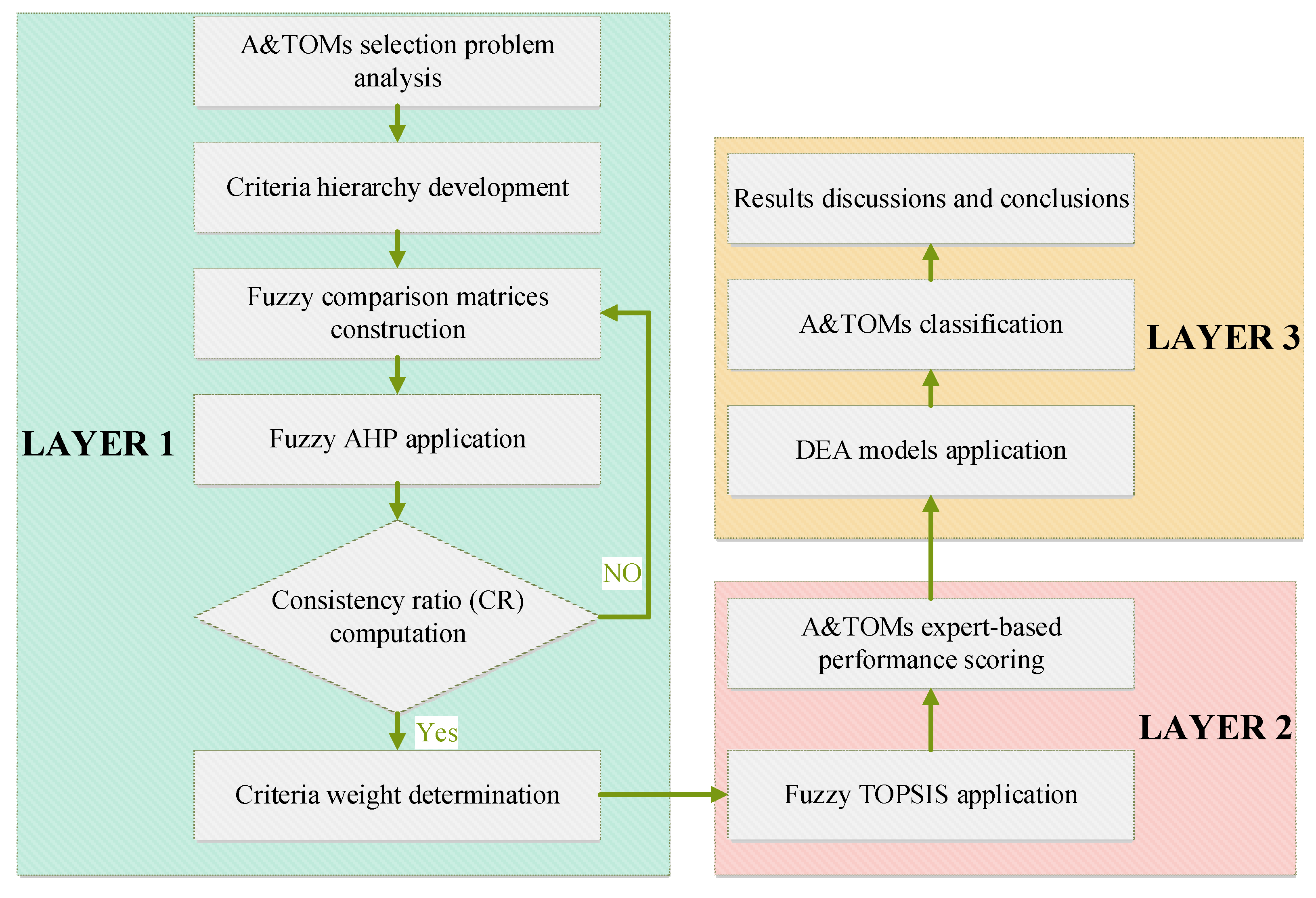
Figure 2.
TFN membership function.

Figure 3.
Criteria hierarchy.

Figure 4.
Criteria linguistics comparison.

Figure 5.
Data envelopment analysis model.
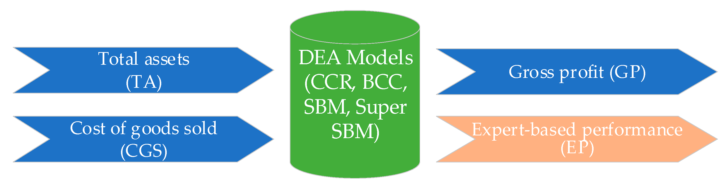
Figure 6.
A&TOMs classification.

Table 1.
A&TOMs selection criteria.
| No. | Authors | Year | Criteria | ||||||
|---|---|---|---|---|---|---|---|---|---|
| Cost | Quality | Logistics Service | Production/Sale Service | Technology | Business/Branding Management | Environmental Production System | |||
| 1 | Çebi and Bayraktar [14] | 2003 | X | X | X | ||||
| 2 | Shen J. et al. [6] | 2012 | X | X | X | X | X | X | |
| 3 | Prusak et al. [15] | 2013 | X | X | X | X | X | ||
| 4 | Dursun, M. and Karsak, E.E. [16] | 2013 | X | X | X | X | |||
| 5 | Karsak, E.E. and Dursun, M. [17] | 2015 | X | X | X | X | |||
| 6 | Banaeian, N. et al. [18] | 2015 | X | X | X | X | |||
| 7 | Jing, S.L. [19] | 2018 | X | X | X | X | |||
| 8 | Nong, N.-M.T., and Ho, P.T. [3] | 2019 | X | X | X | X | X | ||
| 9 | Bakhat, R. and Rajaa, M. [20] | 2019 | X | X | X | X | |||
| 10 | Li, Y. et al. [21] | 2019 | X | X | X | X | X | ||
| 11 | Ulutaş, A. [22] | 2019 | X | X | X | X | X | ||
| 12 | Nakiboglu, G. and Bulgurcu, B. [23] | 2020 | X | X | X | X | |||
| 13 | Govindan, K. et al. [24] | 2020 | X | X | X | ||||
| 14 | Yang, Y. and Wang, Y. [25] | 2020 | X | X | X | X | X | ||
| 15 | Ulutaş, A. et al. [26] | 2021 | X | X | X | X | |||
Table 2.
Alternative selection MCDM method applications.
| No. | Authors | Year | Methods | |||||
|---|---|---|---|---|---|---|---|---|
| AHP | ANP | TOPSIS | Other MCDM | DEA | Mathematical Model | |||
| 1 | Çebi and Bayraktar [14] | 2003 | X | |||||
| 2 | Ravi, V. et al. [27] | 2005 | X | X | ||||
| 3 | Lee et al. [28] | 2010 | X | X | ||||
| 4 | Chin-Nung, Liao [11] | 2012 | X | X | ||||
| 5 | Shen et al. [6] | 2012 | X | X | ||||
| 6 | Prusak et al. [15] | 2013 | X | |||||
| 7 | Yu et al. [5] | 2013 | X | X | ||||
| 8 | Jayant, A. et al. [29] | 2014 | X | X | ||||
| 9 | Taylan et al. [4] | 2014 | X | X | ||||
| 10 | Oztaysi, B. [42] | 2014 | X | X | ||||
| 11 | Tavana, M. et al. [41] | 2015 | X | X | ||||
| 12 | Banaeian, N. et al. [18] | 2015 | X | X | ||||
| 13 | Mangla et al. [30] | 2015 | X | |||||
| 14 | Bouzon, M. et al. [31] | 2016 | X | |||||
| 15 | Li et al. [32] | 2016 | X | X | ||||
| 16 | Otay et al. [33] | 2017 | X | X | ||||
| 17 | Mousavi-Nasab et al. [43] | 2017 | X | X | X | |||
| 18 | Zarbakhshnia et al. [44] | 2018 | X | |||||
| 19 | Mushtaq, F. et al. [34] | 2018 | X | |||||
| 20 | Suganthi, L. et al. [35] | 2018 | X | X | X | |||
| 21 | Azimifard et al. [36] | 2018 | X | X | ||||
| 22 | Wang et al. [37] | 2019 | X | X | X | |||
| 23 | Govindan, K. et al. [24] | 2019 | X | X | ||||
| 24 | Rashidi et al. [10] | 2019 | X | X | ||||
| 25 | Wang et al. [49] | 2019 | X | X | ||||
| 26 | Ebrahimi et al. [50] | 2020 | X | |||||
| 27 | Ghavami et al. [38] | 2020 | X | X | ||||
| 28 | Liu et al. [39] | 2020 | X | X | ||||
| 29 | Solangi et al. [40] | 2021 | X | X | ||||
| 30 | Carvalho et al. [51] | 2021 | X | |||||
| 31 | This paper | 2021 | X | X | X | |||
Table 3.
Importance intensity and the position of TFN are distributed.
| Importance Intensity | Definition | Triangular Fuzzy Number |
|---|---|---|
| 1 | Equal importance | (1, 1, 1) |
| 2 | Lightly importance | (1, 2, 3) |
| 3 | Weak importance | (2, 3, 4) |
| 4 | Preferable | (3, 4, 5) |
| 5 | Importance | (4, 5, 6) |
| 6 | Fairly importance | (5, 6, 7) |
| 7 | Highly importance | (6, 7, 8) |
| 8 | Strongly importance | (7, 8, 9) |
| 9 | Extremely importance | (8, 9, 9) |
Table 4.
Assessment of linguistic levels of the alternatives in the fuzzy TOPSIS model.
| Linguistic Evaluation Levels | Triangular Fuzzy Number |
|---|---|
| Too poor | (1, 1, 1) |
| Very poor | (1, 2, 3) |
| Poor | (2, 3, 4) |
| Bad | (3, 4, 5) |
| Medium | (4, 5, 6) |
| Rather | (5, 6, 7) |
| Good | (6, 7, 8) |
| Very good | (7, 8, 9) |
| Perfect | (8, 9, 9) |
Table 5.
Related research’s DEA inputs and outputs.
| Authors | Year | Input Factors | Output Factors |
|---|---|---|---|
| Hung and Lu [56] | 2009 | Equity Assets Employees | Profit Revenue EPS |
| Yuan et al. [57] | 2010 | Salary Investments Staff | Sales volume Total revenue |
| Li, M.-D. et al. [58] | 2014 | Total assets Costs Total operating | Operating income Earnings per share Net profit |
| Chen and Li [59] | 2017 | Business costs Number of workers Total assets | Corporate income Return on equity Gross profit |
Table 6.
Correlation coefficient.
| Correlation Coefficient | Degree |
|---|---|
| >0.8 | Very high |
| 0.6–0.8 | High |
| 0.4–0.6 | Medium |
| 0.2–0.4 | Low |
| <0.2 | Very Low |
Table 7.
Main criteria fuzzy pairwise comparison matrix.
| Criteria | C1 | C2 | C3 | C4 |
|---|---|---|---|---|
| C1 | (1, 1, 1) | (5, 6, 7) | (7, 8, 9) | (7, 8, 9) |
| C2 | (1/7, 1/6, 1/5) | (1, 1, 1) | (3, 4, 5) | (3, 4, 5) |
| C3 | (1/9, 1/8, 1/7) | (1/5, 1/4, 1/3) | (1, 1, 1) | (1, 2, 3) |
| C4 | (1/7, 1/8, 1/9) | (1/5, 1/4, 1/3) | (1/3, 1/2, 1) | (1, 1, 1) |
Notation: Financial ability (C1), quality assurance (C2), service commitment (C3), technological superiority (C4).
Table 8.
Main criteria non-fuzzy comparison matrix.
| Criteria | C1 | C2 | C3 | C4 |
|---|---|---|---|---|
| C1 | 1 | 5.916 | 7.937 | 7.937 |
| C2 | 0.169 | 1 | 3.873 | 3.873 |
| C3 | 0.126 | 0.258 | 1 | 1.732 |
| C4 | 0.126 | 0.258 | 0.577 | 1 |
| 1.421 | 7.433 | 13.388 | 14.542 |
Notation: Authors’ calculation.
Table 9.
Main criteria normalization comparison matrix and priority vector.
| Criteria | C1 | C2 | C3 | C4 | Priority Vector |
|---|---|---|---|---|---|
| C1 | 0.704 | 0.796 | 0.593 | 0.546 | 0.660 |
| C2 | 0.119 | 0.135 | 0.289 | 0.266 | 0.202 |
| C3 | 0.089 | 0.035 | 0.075 | 0.119 | 0.079 |
| C4 | 0.089 | 0.035 | 0.043 | 0.069 | 0.059 |
Notation: Authors’ calculation.
Table 10.
Main criteria geometric mean.
| Criteria | Geometric Mean |
|---|---|
| C1 | (3.956, 4.427, 4.880) |
| C2 | (1.065, 1.278, 1.495) |
| C3 | (0.386, 0.500, 0.615) |
| C4 | (0.293, 0.354, 0.467) |
| SUM | (5.701, 6.558, 7.457) |
| SUM−1 | (0.134, 0.152, 0.175) |
Notation: Authors’ calculation.
Table 11.
Main criteria fuzzy weight.
| Criteria | Fuzzy Weight |
|---|---|
| C1 | (0.531, 0.675, 0.856) |
| C2 | (0.143, 0.195, 0.262) |
| C3 | (0.052, 0.076, 0.108) |
| C4 | (0.039, 0.054, 0.082) |
Notation: Authors’ calculation.
Table 12.
Main criteria and sub-criteria fuzzy weight.
| Criteria | Fuzzy Weight | Sub-Criteria | Fuzzy Weight |
|---|---|---|---|
| C1 | (0.531, 0.675, 0.856) | C1-1 | (0.324, 0.550, 0.856) |
| C1-2 | (0.242, 0.368, 0.625) | ||
| C1-3 | (0.059, 0.082, 0.120) | ||
| C2 | (0.143, 0.195, 0.262) | C2-1 | (0.540, 0.707, 0.916) |
| C2-2 | (0.165, 0.223, 0.305) | ||
| C2-3 | (0.055, 0.070, 0.093) | ||
| C3 | (0.052, 0.076, 0.108) | C3-1 | (0.507, 0.682, 0.905) |
| C3-2 | (0.173, 0.236, 0.328) | ||
| C3-3 | (0.063, 0.082, 0.112) | ||
| C4 | (0.039, 0.054, 0.082) | C4-1 | (0.562, 0.709, 0.872) |
| C4-2 | (0.181, 0.231, 0.309) | ||
| C4-3 | (0.052, 0.06, 0.077) |
Notation: Authors’ calculation.
Table 13.
Sub-criteria final fuzzy weight.
| Sub-Criteria | Direction | Final Fuzzy Weight |
|---|---|---|
| C1-1 | Minimize | (0.172, 0.371, 0.733) |
| C1-2 | Minimize | (0.128, 0.248, 0.535) |
| C1-3 | Maximize | (0.031, 0.055, 0.103) |
| C2-1 | Maximize | (0.077, 0.138, 0.240) |
| C2-2 | Maximize | (0.024, 0.043, 0.080) |
| C2-3 | Minimize | (0.008, 0.014, 0.024) |
| C3-1 | Minimize | (0.026, 0.052, 0.098) |
| C3-2 | Maximize | (0.009, 0.018, 0.035) |
| C3-3 | Minimize | (0.003, 0.006, 0.012) |
| C4-1 | Maximize | (0.022, 0.038, 0.071) |
| C4-2 | Minimize | (0.007, 0.012, 0.025) |
| C4-3 | Minimize | (0.002, 0.003, 0.006) |
Notation: Authors’ calculation.
Table 14.
Ideal, negative ideal and relative gaps-degree.
| DMU | Ideal Gap | Negative Ideal Gap | Relative Gaps-Degree |
|---|---|---|---|
| A&TOM-01 | 0.125 | 0.122 | 0.495 |
| A&TOM-02 | 0.127 | 0.156 | 0.55 |
| A&TOM-03 | 0.135 | 0.116 | 0.46 |
| A&TOM-04 | 0.133 | 0.186 | 0.582 |
| A&TOM-05 | 0.173 | 0.141 | 0.449 |
| A&TOM-06 | 0.072 | 0.173 | 0.706 |
| A&TOM-07 | 0.091 | 0.179 | 0.663 |
| A&TOM-08 | 0.034 | 0.219 | 0.867 |
| A&TOM-09 | 0.191 | 0.053 | 0.216 |
| A&TOM-10 | 0.180 | 0.087 | 0.327 |
| A&TOM-11 | 0.208 | 0.053 | 0.204 |
| A&TOM-12 | 0.074 | 0.196 | 0.725 |
| A&TOM-13 | 0.201 | 0.054 | 0.212 |
| A&TOM-14 | 0.157 | 0.125 | 0.443 |
| A&TOM-15 | 0.090 | 0.165 | 0.648 |
Notation: Authors’ calculation.
Table 15.
Relative gaps-degree average value.
| DMU | Relative Gaps-Degree | Average Relative Gaps-Degree | |||
|---|---|---|---|---|---|
| Decision Maker 1 | Decision Maker 2 | … | Decision Maker 20 | ||
| A&TOM-01 | 0.564 | 0.504 | … | 0.495 | 0.479 |
| A&TOM-02 | 0.505 | 0.302 | … | 0.550 | 0.465 |
| A&TOM-03 | 0.538 | 0.560 | … | 0.460 | 0.542 |
| A&TOM-04 | 0.539 | 0.394 | … | 0.582 | 0.59 |
| A&TOM-05 | 0.322 | 0.199 | … | 0.449 | 0.482 |
| A&TOM-06 | 0.570 | 0.506 | … | 0.706 | 0.492 |
| A&TOM-07 | 0.553 | 0.506 | … | 0.663 | 0.447 |
| A&TOM-08 | 0.608 | 0.439 | … | 0.867 | 0.602 |
| A&TOM-09 | 0.723 | 0.764 | … | 0.216 | 0.51 |
| A&TOM-10 | 0.552 | 0.560 | … | 0.327 | 0.521 |
| A&TOM-11 | 0.331 | 0.418 | … | 0.204 | 0.385 |
| A&TOM-12 | 0.109 | 0.361 | … | 0.725 | 0.488 |
| A&TOM-13 | 0.552 | 0.495 | … | 0.212 | 0.435 |
| A&TOM-14 | 0.816 | 0.613 | … | 0.443 | 0.544 |
| A&TOM-15 | 0.391 | 0.376 | … | 0.648 | 0.506 |
Notation: Authors’ calculation.
Table 16.
DEA model’s inputs and outputs.
| Input | Output | |||
|---|---|---|---|---|
| DMU | TA | CGS | GP | EP |
| A&TOM-01 | 2,849,534 | 2,976,423 | 620,183 | 0.478888 |
| A&TOM-02 | 751,665 | 548,469 | 103,532 | 0.465032 |
| A&TOM-03 | 593,077 | 1,353,033 | 261,845 | 0.541631 |
| A&TOM-04 | 2,820,761 | 2,708,641 | 63,57 | 0.590117 |
| A&TOM-05 | 1,272,238 | 1,222,601 | 202,328 | 0.481764 |
| A&TOM-06 | 921,297 | 813,050 | 103,377 | 0.492412 |
| A&TOM-07 | 347,846 | 252,525 | 49,149 | 0.446507 |
| A&TOM-08 | 2,977,976 | 1,585,016 | 469,328 | 0.601649 |
| A&TOM-09 | 1,215,003 | 1,807,548 | 115,294 | 0.509697 |
| A&TOM-10 | 10,013 | 106,533 | 12,670 | 0.520968 |
| A&TOM-11 | 611,927 | 537,551 | 158,247 | 0.384776 |
| A&TOM-12 | 13,082 | 217,738 | 859 | 0.487503 |
| A&TOM-13 | 457,318 | 653,648 | 219,147 | 0.434678 |
| A&TOM-14 | 195,698 | 394,735 | 75,808 | 0.544012 |
| A&TOM-15 | 989,736 | 622,793 | 206,520 | 0.505728 |
Notation: Authors’ collection.
Table 17.
The results of correlation coefficient.
| TA | CGS | TR | GP | EP | |
|---|---|---|---|---|---|
| TA | 1 | 0.880857 | 0.997829 | 0.687256 | 0.480023 |
| CS | 0.817037 | 0.690424 | 0.820937 | 0.793349 | 0.346464 |
| CGS | 0.880857 | 1 | 0.892835 | 0.620686 | 0.40558 |
| GP | 0.687256 | 0.620686 | 0.697232 | 1 | 0.121578 |
| EP | 0.480023 | 0.40558 | 0.475781 | 0.121578 | 1 |
Notation: Authors’ calculation.
Table 18.
A&TOMs ranks with nine DEA models.
| Supplier | CCR-I | CCR-O | BCC-I | BCC-O | SBM-I-C | SBM-O-C | Super SBM-I-C | Super SBM-I-V | Super SBM-O-C |
|---|---|---|---|---|---|---|---|---|---|
| A&TOM-01 | 11 | 11 | 1 | 1 | 9 | 14 | 9 | 7 | 14 |
| A&TOM-02 | 10 | 10 | 12 | 15 | 11 | 8 | 11 | 13 | 8 |
| A&TOM-03 | 6 | 6 | 1 | 1 | 4 | 10 | 4 | 13 | 8 |
| A&TOM-04 | 15 | 15 | 9 | 8 | 15 | 15 | 15 | 9 | 15 |
| A&TOM-05 | 12 | 12 | 13 | 13 | 12 | 11 | 12 | 12 | 11 |
| A&TOM-06 | 13 | 13 | 14 | 12 | 13 | 9 | 13 | 14 | 9 |
| A&TOM-07 | 7 | 7 | 10 | 14 | 10 | 4 | 10 | 11 | 4 |
| A&TOM-08 | 5 | 5 | 1 | 1 | 7 | 7 | 7 | 4 | 7 |
| A&TOM-09 | 14 | 14 | 15 | 11 | 14 | 12 | 14 | 15 | 12 |
| A&TOM-10 | 1 | 1 | 1 | 1 | 1 | 1 | 1 | 1 | 1 |
| A&TOM-11 | 4 | 4 | 8 | 10 | 6 | 5 | 6 | 8 | 5 |
| A&TOM-12 | 9 | 9 | 11 | 9 | 8 | 13 | 8 | 10 | 13 |
| A&TOM-13 | 1 | 1 | 1 | 1 | 1 | 1 | 2 | 5 | 2 |
| A&TOM-14 | 8 | 8 | 1 | 1 | 5 | 6 | 5 | 2 | 6 |
| A&TOM-15 | 1 | 1 | 1 | 1 | 1 | 1 | 3 | 6 | 3 |
Notation: Authors’ calculation.
Publisher’s Note: MDPI stays neutral with regard to jurisdictional claims in published maps and institutional affiliations. |
© 2021 by the authors. Licensee MDPI, Basel, Switzerland. This article is an open access article distributed under the terms and conditions of the Creative Commons Attribution (CC BY) license (https://creativecommons.org/licenses/by/4.0/).
Share and Cite
MDPI and ACS Style
Wang, C.-N.; Pham, T.-D.T.; Nhieu, N.-L. Multi-Layer Fuzzy Sustainable Decision Approach for Outsourcing Manufacturer Selection in Apparel and Textile Supply Chain. Axioms 2021, 10, 262. https://doi.org/10.3390/axioms10040262
AMA Style
Wang C-N, Pham T-DT, Nhieu N-L. Multi-Layer Fuzzy Sustainable Decision Approach for Outsourcing Manufacturer Selection in Apparel and Textile Supply Chain. Axioms. 2021; 10(4):262. https://doi.org/10.3390/axioms10040262
Chicago/Turabian StyleWang, Chia-Nan, Thuy-Duong Thi Pham, and Nhat-Luong Nhieu. 2021. "Multi-Layer Fuzzy Sustainable Decision Approach for Outsourcing Manufacturer Selection in Apparel and Textile Supply Chain" Axioms 10, no. 4: 262. https://doi.org/10.3390/axioms10040262
Note that from the first issue of 2016, this journal uses article numbers instead of page numbers. See further details here.