Article

Techniques for Classifying Seabed Morphology and Composition on a Subtropical-Temperate Continental Shelf

by
Michelle Linklater
*,
Timothy C. Ingleton
,
Michael A. Kinsela
,
Bradley D. Morris
,
Katie M. Allen
,
Michael D. Sutherland
and
David J. Hanslow
Waters, Wetlands and Coasts, Science Division, New South Wales Office of Environment and Heritage, 59-61 Goulburn St, Sydney NSW 2000, Australia
*
Author to whom correspondence should be addressed.
Geosciences 2019, 9(3), 141; https://doi.org/10.3390/geosciences9030141
Submission received: 13 December 2018 / Revised: 15 March 2019 / Accepted: 19 March 2019 / Published: 22 March 2019
(This article belongs to the Special Issue Geological Seafloor Mapping)

Abstract

:
In 2017, the New South Wales (NSW) Office of Environment and Heritage (OEH) initiated a state-wide mapping program, SeaBed NSW, which systematically acquires high-resolution (2–5 m cell size) multibeam echosounder (MBES) and marine LiDAR data along more than 2000 km of the subtropical-to-temperate southeast Australian continental shelf. This program considerably expands upon existing efforts by OEH to date, which have mapped approximately 15% of NSW waters with these technologies. The delivery of high volumes of new data, together with the vast repository of existing data, highlights the need for a standardised, automated approach to classify seabed data. Here we present a methodological approach with new procedures to semi-automate the classification of high-resolution bathymetry and intensity (backscatter and reflectivity) data into a suite of data products including classifications of seabed morphology (landforms) and composition (substrates, habitats, geomorphology). These methodologies are applied to two case study areas representing newer (Wollongong, NSW) and older (South Solitary Islands, NSW) MBES datasets to assess the transferability of classification techniques across input data of varied quality. The suite of seabed classifications produced by this study provide fundamental baseline data on seabed shape, complexity, and composition which will inform regional risk assessments and provide insights into biodiversity and geodiversity.

1. Introduction

Understanding the form and nature of the seabed is a critical first step in managing coastal and marine ecosystems [1,2]. Bathymetry and intensity (backscatter and reflectivity) data sourced from remote-sensing platforms such as multibeam echosounders (MBES) and marine LiDAR contribute crucial information for hydrographic charting and are used to derive abiotic variables which can act as a surrogate for the occurrence and abundance of benthic and pelagic biota [3,4,5]. Bathymetry data, intensity data, and their derivatives can be integrated with ground-truthing data to predict distributions of biota and substrates across broad spatial scales and create continuous surfaces of predicted species of sediment distributions and categorical maps of geomorphic features and biotopes [1,6]. Such maps are integral for marine spatial planning [7,8], fisheries resource assessments [9], marine biodiversity assessments [10], and hazard risk assessments [11,12]. The principal of ‘collect once, use many times’ is paramount to the collection of bathymetric and intensity data, due to the high cost and effort of data collection and processing, and because it is recognised as fundamental baseline information for these diverse coastal and marine management applications [1,13].
Despite the broad array of applications of bathymetry and intensity data, vast amounts of the seabed remain unmapped [14]. Global coverage of bathymetry data is available through derived altimetry methods, however the resolution of these grids (30 arc-second grid cells, ~1 km at the equator) are considered too coarse for most regional or local management applications and it is estimated that less than 18% of the earth’s surface is mapped with echosounding equipment [14,15]. A concerted effort involving the NIPPON Foundation and the general bathymetric chart of the oceans (GEBCO) has recently embarked upon ‘Seabed 2030’, which aims to map the entire world’s oceans with higher resolution technologies (100–800 m resolution grids) by 2030 to address this substantial gap in knowledge [14]. On a national scale, recent initiatives including the Australian Department of Defence SEA2400 [16], AusSeabed [http://www.ausseabed.gov.au/home], and Seamap Australia [https://seamapaustralia.org/] programs aim to collect, collate, and consolidate mapping efforts within Australian waters and charting territories. These initiatives highlight the prioritisation of hydrographic charting acquisition and the recognition of the benefits of bathymetric data (see Supplementary Materials) and its associated products to national and international interests.
As the volume of high-resolution seabed data increases globally, there is a growing interest in automated approaches to process and classify seabed data [17]. Manual classification of seabed data has been a common approach to date, however automated approaches including geostatistical, object-based, and machine learning methods are increasingly being developed as they offer benefits of repeatability and reduced subjectivity [17,18]. In a comparison of the abovementioned methodologies to the application of substrate mapping, Diesing et al. [17] found statistically similar outputs across manual and automated approaches. Similarly, in comparing autoclassification and cognitive interpretation techniques for characterising seabed geomorphology from marine LiDAR data, Finkl and Makowski [19] found that interactive supervised autoclassification methods could accurately capture known seabed topography. While automated approaches offer promising benefits of repeatability, the application of these classification techniques to seabed mapping remains a developing field of study and expert involvement is still required to design the classification and validation framework and assess the quality of the output classification.
The discipline of marine geomorphometry is concerned with quantitative seabed terrain analysis and spans the creation, interrogation, and classification of surface forms and features [20]. It encapsulates the derivation of statistical measures (such as slope) from bathymetric data, referred to as general geomorphometry, and the extraction of discrete features (such as landforms), referred to as specific geomorphometry [18]. In the applications of general geomorphometry, derivatives of slope, curvature, rugosity, and topographic position are among the most common variables calculated in studies characterising the marine environment [21]. Derivatives from bathymetric data have typically been generated based on window scales of 3 × 3 as this is typically the input grid size default setting of spatial software packages [22], however there are movements toward multiscale analysis [23,24]. This allows users to explore the function of variables at a range of fine to broad scales to determine what scales most effectively relate to the target of interest [25]. The capacity for generating multiscale variables has been incorporated into recent releases of marine geomorphometry toolboxes, including Benthic Terrain Modeler [26] and Geomorphometry and Gradients Metrics Toolbox [27], allowing users to readily generate derivatives at a range of window sizes to explore scales most relevant to their focus of study.
Scale of analysis is also an important consideration for specific geomorphometry, where landforms and geomorphic objects are defined [18]. The implications of landform mapping at varied scales is discussed by Picard et al. [28] whereby automated approaches developed for the classification of seabed landforms at an international scale (sourced from Reference [29]) are adopted and modified for application to regional scale landform mapping. This study by Picard et al. [28] highlights the inherent relationship between the scale of features mapped and the spatial resolution of input data, and the importance of MBES in resolving finer scale geomorphic features indistinguishable from coarser global bathymetry models.
As the definition of features and surface parameters pertain to the scale of analysis selected [30], seascapes can be interrogated and classified at hierarchical levels to meet user requirements [31]. This hierarchical approach has been adopted in a number of seabed classification systems [32,33,34,35,36], whereas other widely adopted classification systems, such as the International Hydrographic Organisation (IHO) undersea feature names [37] and hydrographic dictionary [38] aim to be largely scale-independent.
In applications of specific geomorphometry, where discrete landforms are identified, the method of classification is inherently tied to a classification scheme which outlines the definitions for the feature of interest. Definitions of landform terms are available in schemes which focus on seabed features, such as the IHO undersea feature names [37] and hydrographic dictionary [38], as well as broader schemes which incorporate geomorphology, biota, and substrates, such as the Coastal and Marine Ecological Classification Standard [39]. The separation of morphological terms, which are objective descriptions of feature shape and form, from geomorphic terms, which infer feature origin and evolution, has recently been presented by Dove et al. [40] as a two-stage classification framework. This definition of morphological units aligns to the definition of ‘landforms’ presented by Evans et al. [18], which defines landforms objects as grouped areas of ‘surface elements’ representing homogenous gradients, aspects, or curvatures. Variations of such features may be recognised elsewhere as geomorphrons [41], geofeatures [42], or bathymorphrons [43]. The interpretation of geomorphic features is, in turn, associated with the classified landforms to infer processes shaping feature evolution [18,40], and such features may be recognised as geomorphic units (e.g., Reference [29]) or geoforms (e.g., Reference [39]).
In Australia, a unified national classification scheme for landforms and geomorphic features focusing on continental shelf environments is currently in development [42,44]. The draft framework aims to adopt the two-stage classification of morphology and geomorphology presented in Dove et al. [40], with other components such as biota and substrate characterisations classed as separate entities with nested hierarchical terms. This flexible approach can be modified to match the availability of input data and scale [44] with terms for geofeatures aiming to be scale-independent [42]. The unified scheme attempts to bring together the diverse suite of classification methods and schemes currently employed around Australia (e.g., References [45,46,47,48,49]).
Within New South Wales (NSW) in southeastern Australia (Figure 1), the Office of Environment and Heritage (OEH) has mapped 15% of state waters (from the coast to 3 nm limit) with high-resolution bathymetry and intensity (backscatter and reflectivity) data. The acquisition of this data was collected across the continental shelf zone with a range of technologies including multibeam echosounders, interferometric sidescan sonar, and marine LiDAR. Seabed classifications produced by OEH from this mapping effort to date have been limited to manual digitisation of reef extent, subclassified into three depth zones (0–25, 25–60, and greater than 60 m depth) [45,50] and the digitisation of aerial imagery [51]. This habitat data was critical for marine park zoning review assessments (e.g., References [52,53]) and has been useful in understanding the stratification of fish assemblages across the shelf [54,55]. The development of standardised national nomenclature for shelf features [42,44] and the availability of tools for exploring marine geomorphometry [18,26] highlights the opportune timing for OEH to develop improved classification methodologies which incorporate recent progress in classification schemes and methodologies.

1.1. SeaBed NSW

SeaBed NSW was initiated in 2017 as a four-year state-wide seabed mapping program, funded in conjunction with legislative coastal reforms undertaken in NSW, which identified the need for increased understanding of coastal and marine environments [56]. The program, conducted by OEH, aims to collect and deliver baseline information on seabed morphology and composition and represents a considerable expansion of seabed mapping effort in NSW state waters. Data delivered under SeaBed NSW will support the implementation of the NSW legislative framework which includes the Coastal Management Act 2016, State Environmental Planning Policy (Coastal Management) 2018, Coastal Management Manual, and Marine Estate Management Act 2014.
The new framework of legislative reforms introduced in NSW identifies the need to mitigate current and future risks to land caused by coastal hazards, which include coastal erosion, recession, instability, and inundation (Coastal Management Act 2016, Part 1, Section 4). The new framework furthermore incorporates the concept of sediment compartments (as defined for Australia by References [57,58]), and encourages local government areas to consider coastal erosion within the context of sediment movement between and within adjacent sediment compartments (Coastal Management Act 2016, Schedule 1). This recognition of sediment compartments allows council areas to account for sediment sharing between jurisdictions and assists in managing areas vulnerable to coastal erosion [12].
To aid in localised assessments of vulnerability to coastal hazards such as erosion and inundation, SeaBed NSW aims to collect detailed information on the nearshore and offshore seabed to support coastal hazard studies and inform decision-making processes. Airborne marine LiDAR and MBES systems will collect bathymetry and intensity (backscatter and reflectivity data) targeted to the 0–50 m depth range which is most important for understanding coastal sediment connectivity and transport. Airborne marine LiDAR will be utilised to map the nearshore zone (to approximately 30 m depth), supplemented with MBES in deeper waters offshore (to approximately 50 m depth). Sediment sampling and towed underwater video will be collected to ground-truth remotely-sensed data. The progress of the program to date has resulted in the successful acquisition of state-wide marine LiDAR for the entire NSW coastline [59] and the completed mapping of the Wollongong compartment in the Illawarra region south of Sydney using MBES (Figure 1).
Regional-scale state-wide assessments of exposure to coastal erosion and inundation have been performed by OEH along the NSW coast, which have identified the relative risk of open coast beaches and estuaries to present-day and future coastal hazards [11,12,60]. These regional-scale assessments utilised best-available data, however as much of the state waters were unmapped in high-resolution, the parameterisation of regional models relied on assumptions of nearshore bathymetry and sediment composition [12]. The high-resolution depth and substrate information collected under the SeaBed NSW program will enable more detailed modelling that more accurately characterises local nearshore sediment dynamics and future coastal response [12,61].
Detailed information on the morphology and composition of the seabed can also inform on the distributions of marine biota [6]. In NSW, terrain variables derived from bathymetry data as well as classifications of seabed geomorphic features have been shown to act as useful surrogates for inferring distributions and abundance of biota and substrates [4,62,63], highlighting the importance of seascape characterisations for management of the marine environment. The existing seabed classification approach of OEH which characterises reef extent does not adequately capture the diversity of reef and soft sediment types that may be present within an area. Furthermore, the manual digitisation of features is less feasible as increased volumes of new high-resolution data are collected under the SeaBed NSW program, together with the vast repository of existing seabed mapping data spanning 14 years of acquisition. Due to the diverse needs of the SeaBed NSW program to address coastal hazard assessments and marine estate management, a broader product suite of seabed classifications utilising automated approaches is required.

1.2. Aims and Objectives

The main aim of this study is to develop a flexible classification framework for characterising seabed morphology and composition for application to the continental shelf setting of southeast Australia. We developed new techniques for classifying seabed morphology using a combination of derived landform and seabed composition surfaces for two discrete sections of the NSW coast ~500 km apart. The MBES data collected from the two case study areas at (1) Wollongong (mapped for SeaBed NSW); and (2) an area of existing coverage at the Solitary Islands (Figure 1) were collected during different time periods and are, generally, of different positional quality (vertical and horizontal). We also present several examples for classifying seabed based on the availability of input validation data as three scenarios including (1) no validation data (seabed textures), (2) limited validation data (seabed substrates, character, and geomorphology), and (3) comprehensive organism or species data (seabed habitat). Data for this third scenario is provided for sponge habitats as presence-only data. These examples are presented within the overall classification framework to elucidate how output products can be integrated together and adapted to meet the availability of validation data. Additionally, an area of previously hand-digitised seabed is compared with the semi-automated surface elements classification over a sub-set area to examine the relative ability of semi-automated and manual techniques for identifying ‘profile reef’ features.
The framework presented in this study was developed from MBES data for 5 m cell size DEM and is repeatable across similar marine environments globally. The techniques are intended to be applied to new data acquired with MBES and marine LiDAR under the SeaBed NSW program and beyond, in addition to existing datasets. The broad suite of seabed classification approaches and techniques presented in this study provide fundamental baseline data on seabed morphology and composition which will inform regional risk assessments and provide insights into biodiversity and geodiversity.

2. Materials and Methods

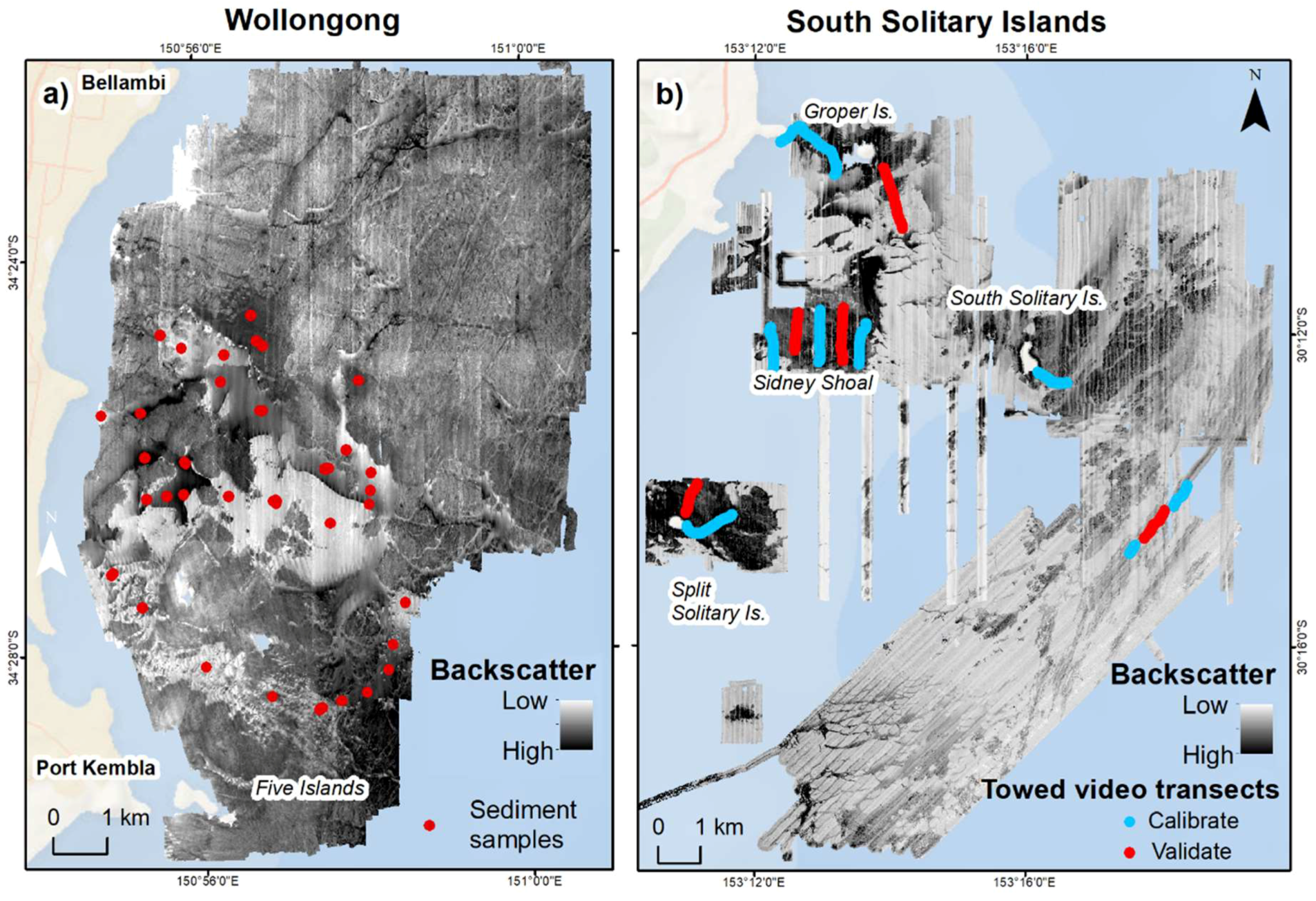
2.1. MBES Data Acquisiton and Processing

MBES data were systematically collected by OEH using two sonar systems—a 200–400 kHz R2Sonic 2022 system (R2Sonic, USA) and a 125 kHz Geoswath interferometric sidescan sonar (Kongsberg, Norway). MBES data for the Wollongong compartment were acquired from August 2016 to May 2017 (R2Sonic and Geoswath) while data at South Solitary Islands was collected during multiple surveys from 2005 to 2012 (Geoswath) (Figure 1 and Figure 2).
Surveys were operated at speeds of 4 to 6 knots with distances between adjacent transects run to achieve 20%–50% overlap and provide a minimum density of 4–5 soundings.m−2. Generally, sonar power, gain, and frequency settings were fixed to maintain relative consistency of the sonar signal across each of the survey areas. In deeper areas, however, power settings for the R2Somic needed to be periodically adjusted to maintain survey specifications. Sound velocity data were collected continuously at the sonar heads and as water column profiles (2–4 times daily) to correct for variability in through-water sound speeds associated with changing densities within the water mass.
For the Wollongong survey area, vessel motion and position were logged using a POS MV (Applanix, Canada) with RTCM DGPS or G2 corrections in real-time. Motion data were post-processed in POSPac using final ephemeris and using either precise point positioning (with 3 min forward-reverse smoothing) or single base-station options to calculate an improved vessel trajectory (root mean square error of XYZ survey errors <0.03 m). Bathymetric soundings were first processed in GS+ (Geoswath) or Hypack (R2Sonic) and then edited and cleaned using CUBE modelling in Qimera/Fledermaus (QPS, Netherlands). Cleaned soundings were then gridded using weighted averaging to produce 2, 5, and 10 m cell size digital elevation models (DEMs). Overlapping R2Sonic and Geoswath data indicated method repeatability of better than 0.08 m and 98% of data for the survey satisfied IHO criteria Order 1B.
For the South Solitary survey area, newer areas (from 2010 onwards) were processed using the methods described above for the Wollongong surveys. For earlier surveys (2005–2009), real-time vessel motion and position were logged using a TSS DMS05 (Teledyne, UK) inertial motion unit set with a 30 s heave window for near-shore small vessel operations. For tidal corrections, an AquaLogger 520PT (Aquatec, UK) pressure sensor was deployed daily within the immediate survey area and later compared with ocean tide data from fixed gauge sites (Manly Hydraulics Laboratory, Sydney) based on timing of the peak being high or low. Real-time motion and tides (relative to Australian Height Datum) were applied in post-processing using GS+ (Geoswath), where raw soundings were filtered using amplitude, box, along, and across track filters to produce a cleaned-sounding dataset for gridding (at 2, 5 and 10 m DEMs).
Total vertical uncertainty (TVU) layers were generated for the Wollongong and South Solitary Islands survey areas to quantify vertical error associated with the final derived bathymetry value for each cell and provide a confidence assessment for the dataset. For the Wollongong surveys, a ‘cleaned-soundings’ dataset (from the CUBE-modelled point editing process) was used to derive a TVU surface based on the same 5 m grid scale for the most recent Wollongong survey (2016–2017) using the R2Sonic. A TVU surface was also generated for an older section of the South Solitary Islands dataset acquired in 2005-8 to enable a comparison of uncertainty between newer and older survey areas.
Backscatter amplitude data from both MBES systems were imported to Fledermaus (FMGT) or Hypack Geocoder where transmit/receive (time), power, gain, and beam pattern corrections were applied. Where different power settings were used during acquisition, backscatter values were adjusted (±5 db) to match backscatter of adjacent areas based on values of overlapping transects. All backscatter data were then combined to create 2, 5, and 10 m grid cell-size greyscale mosaics in Fledermaus and ArcMap (ESRI, USA). Final gridded products are available for download from the Australian Oceanographic Data Network portal (https://portal.aodn.org.au/).

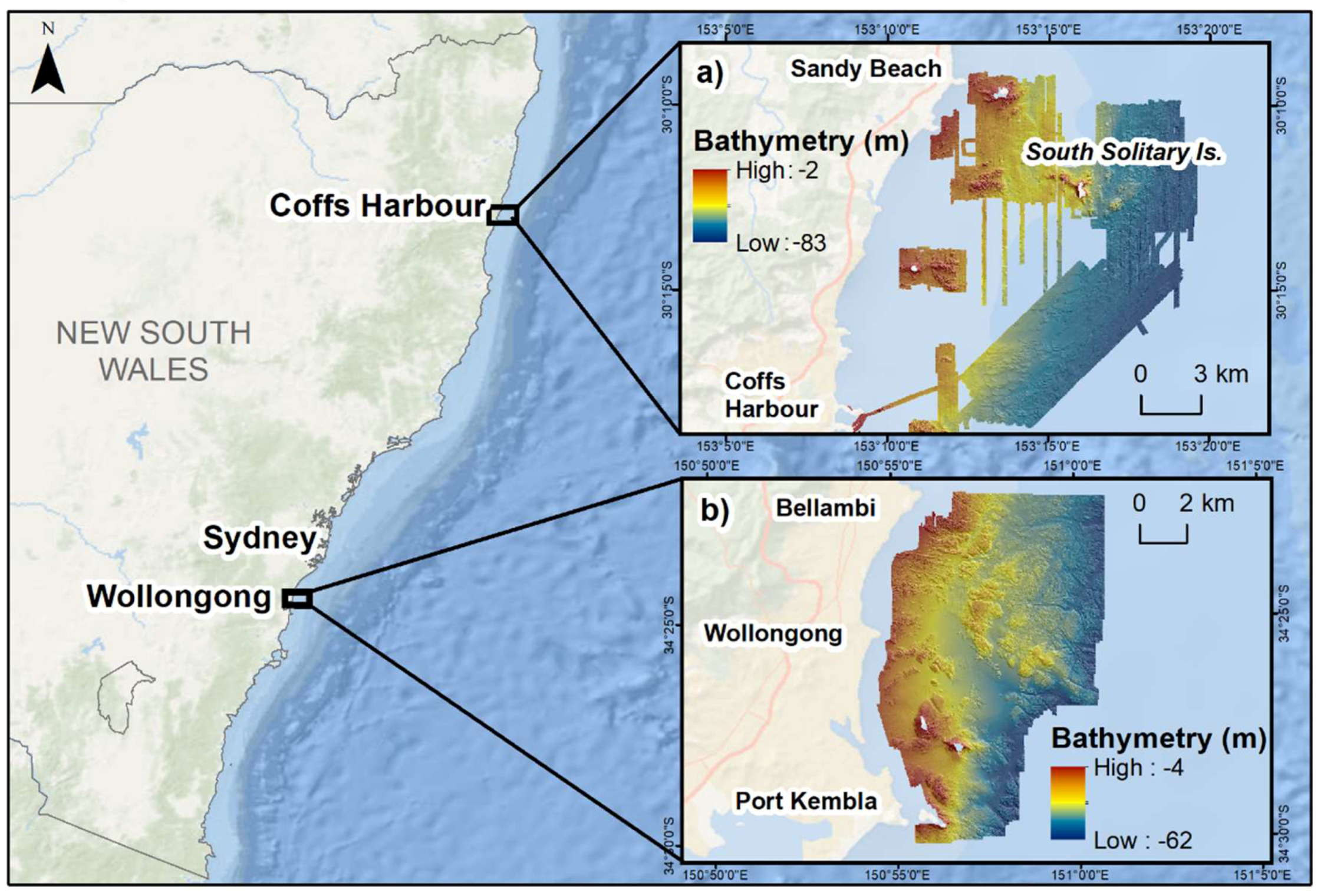
2.2. Digitial Elevation Models

MBES data within each study area were combined to create seamless, high-resolution DEMs (5 m cell size) (Figure 1). The 5 m DEM was selected for analyses as this was the most consistent resolution with existing MBES and marine LiDAR data collected or commissioned by OEH which are typically gridded to 2 m or 5 m cell size. For the Wollongong compartment, a seamless DEM was generated during MBES processing whereas data for South Solitary Islands were combined for this study. DEMs with finer resolutions were resampled to 5 m and grids were mosaicked using Mosaic to New Raster tool in ArcGIS v10.4.

2.3. Ground-Truthing Data Collection and Processing

Sediment grab samples were collected within the Wollongong study area to characterise the seabed substrates and ground-truth the MBES backscatter data (Figure 2a). Sediment samples were collected from RV Bombora from September 2017 to January 2018. A total of 45 sediment samples were recovered from 43 locations between 18 m and 55 m water depth, using Smith McIntyre and Shipek grab samplers deployed via the rear-A crane. The grab samplers were equipped with ultra-short baseline positioning (USBL) to accurately locate the grab position relative to the vessel. The sediment grabs were photographed, subsampled, inspected, and described onboard. Subsamples were collected from the upper 2 cm of the undisturbed grabs using a spoon and were stored in zip-lock bags that were refrigerated and retained for subsequent laboratory analysis.
Sediment texture and composition was described onboard and in the laboratory to determine the character of the samples, in the context of past studies (e.g., Reference [64]) and established models of sediment distribution on the inner-continental shelf in this region [65,66]. The dominant grain size class of each grab sample was identified, and the relative carbonate and mud content of samples was estimated by visual inspection. Quantitative sedimentology and mineralogy analyses are being pursed in collaboration with the University of Wollongong, although such detail is beyond the scope of this study.
Towed underwater video data were collected as validation data for the South Solitary Islands MBES data (Figure 2b). Data were collected aboard RV Glaucus and RV Aquilia from campaigns in 2006, 2008, and 2009. The towfish was equipped with a downward-facing stills camera and forward-facing video camera, with USBL positioning for geolocation. Selected areas of towed video collected in 2006 were not equipped with USBL, and layback was estimated in these areas. Video footage was classified at 10 s intervals using a visual assessment of substrate and biota type and estimated percentage cover. The presence and morphology of sponges were recorded, in addition to algae and selected sessile invertebrates. Detailed methods of video collection and classification are described in [45]. While substrates were classified in the towed video data, this data has not been utilised for substrate classifications in this study. The South Solitary Islands area was treated as an area without validation data for the purposes of the substrate mapping presented in this study, to represent areas of existing data elsewhere on the NSW coast where ground-truthing data is absent.

2.4. Derived Terrain Variables

Terrain variables were derived from the 5 m DEM (Table 1). Slope, aspect, range, standard deviation, curvature, and isobaths (1 m intervals) were calculated with the Spatial Analyst toolbox in ArcGIS v10.4. Additionally, statistical aspect (eastness, northness) and ruggedness (Vector Ruggedness Measure, VRM) were calculated with the Benthic Terrain Modeler extension (BTM) v3.0 [26], and topographic position index surfaces (TPI, also termed slope position) were calculated with the Geomorphometry and Gradient Metrics Toolbox (GGMT) v2.0 [27]. TPI was calculated using GGMT in this study as the BTM tool applies an integer conversion which simplifies the output TPI surface [67]. With the exclusion of ArcGIS software, the BTM and GGMT toolboxes utilised are freely available online. Functions within GGMT are also available with the R package SpatialEco. Tools that are freely available were preferentially utilised in this study to increase accessibility of the method to other user-groups for applications in other survey areas.
The 3-cell rectangular window was selected as the most suitable for ruggedness, standard deviation, and range as these match the window size used for the calculation of slope and aspect by ArcGIS. To explore suitable scales of broadscale and finescale TPI, multiple grids were generated at a range of incremental rectangular window scales from 3 × 3 to 500 × 500 and interrogated to determine which grids collectively captured the features of interest. Scale of mapping for this study is approximately 1:5000 map scale, capturing features that are 10’s of metres in size. The dominant features of interest at that mapping scale include outcropping reefs and inter-reef channels. Finer scale bedform features within the broader plain areas were also explored, but these were of subsidiary interest as these features were low relief (several metres in height) and more apparent within the backscatter. Broader window scales approaching 150 captured greater proportions of the outcropping reef features that were typically digitised with previous manual methods. However, as window scales increased beyond 150, shallow regions of the survey area increasingly appeared as ‘highs’ relative to the surrounding terrain. After interrogation of the TPI surfaces, broadscale and finescale grids with cell radii of 150 and 27 cells, respectively, were determined to be the most relevant scale of analysis for capturing the features observed within the Wollongong study area. The broadscale grid was determined to effectively capture the outcropping features and the finescale grid was determined to effectively capture the depressions and channels within the outcrop surface.

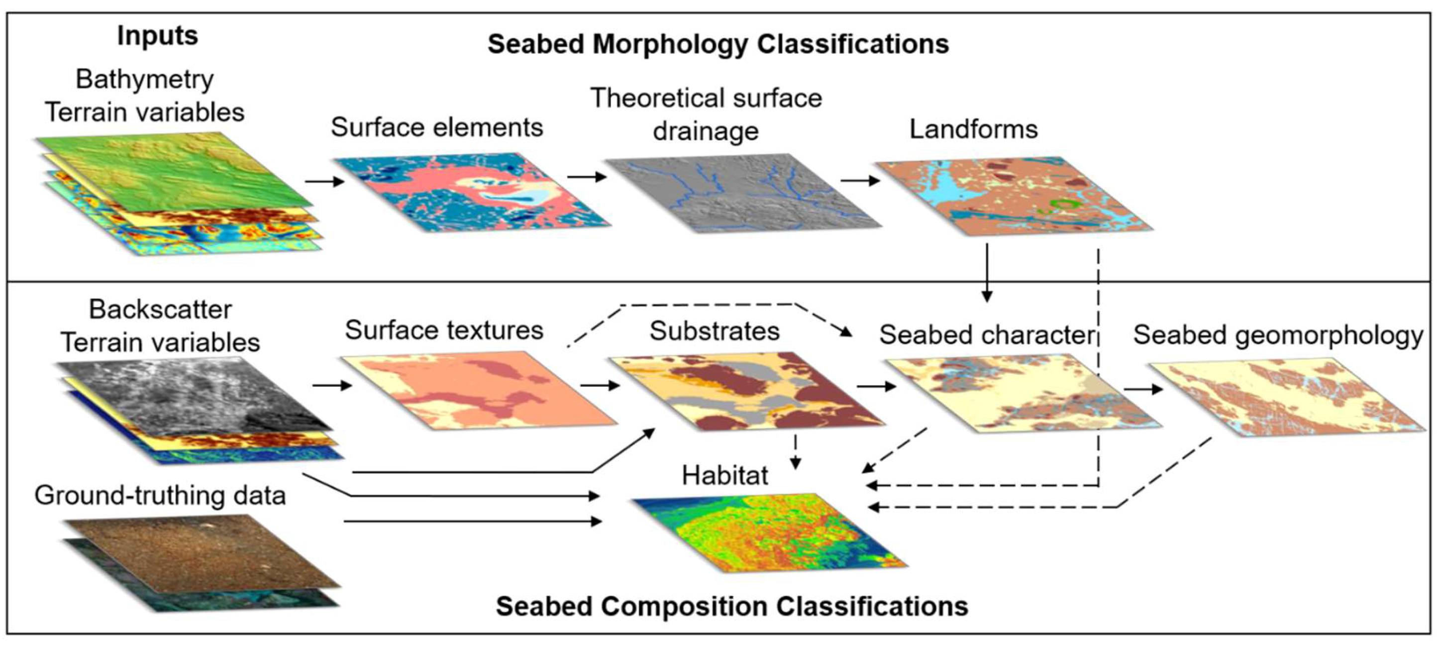
2.5. Classification of Seabed Morphology

Morphological features were identified using a three-stage process, whereby ‘surface elements’ were first delineated, ‘theoretical surface drainage’ patterns were then modelled, and ‘landforms’ were subsequently identified using manual methods. Landforms are bounded segments of a landscape and surface elements are homogenous components of the surface which represent breaks in gradient, aspect, or curvature [18]. The landscape terminology of ‘landforms’ and ‘elements’ were adopted from Evans et al. [18]. Figure 3 represents a schematic of the complete seabed classification workflow, and Table 2 summarises selected classification levels and terms used within the morphology and composition classifications presented in this study.

2.5.1. Surface Elements

Surface elements were classified using a customised dictionary developed for this study (Table 3), implemented using the Classify Benthic Terrain tool in BTM. Variable inputs included broadscale (150 cell radius) and finescale (27 cell radius) TPI layers derived in GGMT, slope derived in ArcGIS Spatial Analyst, and ruggedness (VRM) derived in BTM (Table 1). Slope, broadscale and finescale TPI, and depth are all standard inputs into the BTM classification dictionary [26,67]. However, the focus of SeaBed NSW (0 to 50 m) and the examples considered here (~30 to 80 m) cover relatively narrow depth ranges and depth is not a key component defining the morphological expression of shelf features. For this reason, we present a new application of BTM which substitutes ruggedness for depth in the BTM classification dictionary as it was determined to be the most relevant metric for defining outcropping features. These variables of TPI, slope, and ruggedness have been identified among the most effective variables in capturing topographic structure [68].
Ruggedness was determined to effectively capture outcropping features, which are a prominent feature in the case study area and NSW shelf seascapes more broadly. Other complexity measures including standard deviation, which has been used to define complex outcropping features (e.g., References [28,29]) and range, which is a similar measure of surface complexity, were tested and found to have performed relatively poorly compared to the ruggedness variable in this study area.
The selected threshold value for slope of 10 degrees for the classification dictionary was increased from the value of five degrees in Nichol et al. [42] which captured additional artefacts in the seascape. To determine suitable threshold values for the remaining variables, firstly a multiband image of broadscale TPI, finescale TPI, and ruggedness was created in ArcGIS, and then training areas were identified for the desired surface element classes (e.g., broadscale rugose high, finescale smooth low). A range of supervised classification tools available in ArcGIS, including Support Vector Machine (SVM), Random Trees, ISO cluster, and Maximum Likelihood classifiers, were each tested. Several iterations of training area selection and re-application of each of the model classifiers were run to refine and improve each classification. The outputs of the different classifiers were compared, and the SVM output was determined to best capture the features targeted with the training areas. The selected SVM output was then interrogated using the Identify tool in ArcGIS to determine the threshold values for the classification dictionary.
The ruggedness threshold of 0.0003 used in this study was adjusted to account for artefacts in the Geoswath areas of data within the Wollongong survey area (see Appendix A, Figure A1), and this ruggedness threshold may be modified depending on the quality of the input data. Rugose areas were best represented at a ruggedness threshold of 0.00003 for areas acquired using the R2Sonic, however these captured artefacts in areas acquired with Geoswath and therefore the ruggedness threshold was increased to 0.0003 for this study. For future data collection, lower thresholds for ruggedness, such as 0.00003, is recommended to be applied where possible.

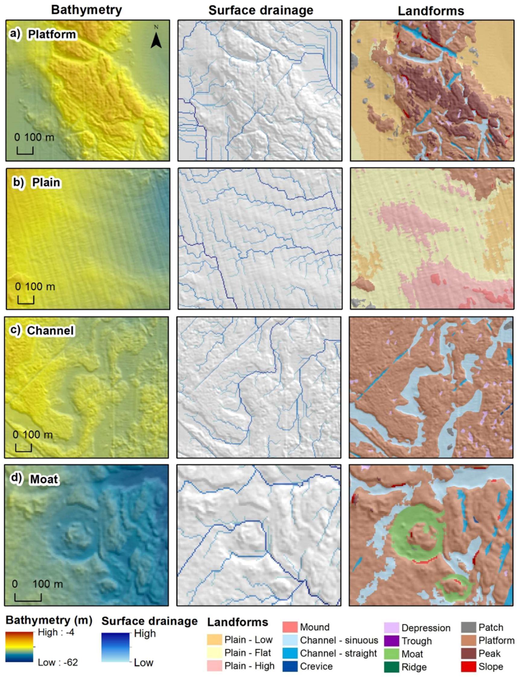
2.5.2. Theoretical Surface Drainage

Theoretical surface drainage was calculated to inform the user on drainage pathways across the seabed surface which would have been active during periods of shelf exposure. The theroetical surface flow layer is used to differentiate surface element classes such as straight and sinuous channels, troughs, and crevices whose definitions relate to sinuosity and surface gradients which are apparent in the modelled drainage layer. This understanding of surface flow direction and accumulation assists geomorphic interpretations which take into account the evolutionary history of the features. Drainage flows were modelled using the Hydrology toolbox in ArcGIS v10.4. The flow direction tool was used to generate a flow direction surface, which was then input into the flow accumulation tool to model drainage pathways. This accumulation surface was log transformed and the data were clipped to 100 m3 to capture dominant flow pathways.

2.5.3. Landforms

Landforms were subsequently classified using the surface elements layer, informed by the surface drainage layer. Landform terms used in this study were sourced from several classification schemes including the draft framework for an Australian standard of the geomorphological classification of reefs [42], the International Hydrographic Organisation standardised undersea feature terms [37] and hydrographic dictionary [38], the coastal and marine ecological classification standard [39], and the British Geological Survey seabed geomorphology classification scheme [40]. The resultant landform classification is consistent with the ‘Morphology’ classification in Dove et al. [40] and ‘Geofeature’ classification in Nichol et al. [42]. Landform definitions and sources are presented in Appendix B, Table A1.
The polygons defined in the surface elements layer form the boundaries of the landform polygons. Two landforms directly relate to the classified surface elements—‘peaks’, which represent ‘Broadscale High Rugose Max’ areas which are the uppermost topographical high areas defined in the broadscale TPI; and ‘slopes’, which are defined as all areas greater than 10 degrees in slope. The remaining landforms required surface elements to be compiled and manually edited to define feature extents. Input surface elements were interrogated using the surface drainage pathways and derived isobaths (1 m intervals) together with terrain profiles conducted to determine feature shape and relief. Manual edits were undertaken in the form of polygon selection and re-labelling, and polygon cutting. Manual editing of the surface element layer can be at the discretion of the user and the feature definition criteria. The approach of manual editing, as undertaken in this study, is outlined below.
Surface elements were aggregated into summarised classes to simplify the editing process. ‘Plane Rugose’, ‘Finescale and Broadscale Low Rugose’, and ‘Finescale and Broadscale High Rugose’ were collated into ‘Rugose outcrops’ which were, in turn, separated into ‘Platforms’, ‘Patch reefs’, and ‘Ridges’. Patch reefs form all isolated rugose outcrops smaller than 6000 m2. ‘Smooth outcrops’ were defined for areas of ‘Finescale or Broadscale High Smooth’. These areas were separated into ‘Mound’ landforms where they occurred as isolated rises or were divided into ‘Plain–High’ or ‘Platforms’ as appropriate. ‘Finescale or Broadscale Low Smooth‘ areas represent ‘Smooth low’ areas, and ‘Plane Smooth’ represent ‘Smooth flat’ areas. Manual edits of these smooth low and flat areas were performed to separate and define areas of ‘Plain–Flat’, ‘Plain–Low’, ‘Depressions’, ‘Crevices’, ‘Channels’, ‘Troughs’, and ‘Moats’ which can occur within and between rugose and smooth outcrops.
The recommended sequence of landform editing, as undertaken in this Wollongong case study area, is as follows: (1) Create new attribute field for landform features and transfer across ‘peaks’ and ‘slopes’ attributes to the landform classification; (2) aggregate all remaining surface elements into summarised terms (e.g., rugose outcrops), as outlined above; (3) identify and re-label channels, troughs, crevices, depressions, and moats that occur within the reef structure. Manually cut channels that occur between and within outcrops to separate from broader plains; (4) identify plains, which occur as broad expanses; (5) identify mounds and ridges, which may comprise smooth or rugose outcrops and occur within plains; (6) identify smooth outcrops which occur within the reef and relabel as ‘platforms’; and (7) select all platform features less than 6000 m2 and re-label as patch reefs.
Smooth, low-profile reef outcrops require greater manual editing which typically comprises re-attributing polygons within the reef surface. This can be performed by extracting the rugose outcrops surface and selecting all smooth outcrop polygons which occur within the rugose outcrops layer. Some low-profile outcrops may need to be digitised (cut) to separate from the surrounding plain if boundaries are not adequately captured by the surface elements classification.
An example of the decision-making process to differentiate channels, troughs, and crevices is outlined below to demonstrate the application of this workflow to selected features. Channels, troughs, and crevices may be initially defined as ‘plane smooth’, ‘smooth low’, or ‘smooth outcrops’ summarised surface elements; and are all defined as elongate depressions. Channels and troughs exhibit a steepening gradient which is evident in the drainage pathways and isobaths, whereas crevices are narrow, may be close-contoured, and are disconnected to dominant drainage pathways. Channels are ‘V’- or ‘U’-shaped, whereas troughs are flat-bottomed, and this channel structure can be determined by conducting 2D surface profiles. The surface drainage pathways can be used to determine sinuosity of the channel to differentiate straight from sinuous channels.

2.6. Classification of Seabed Composition

We produce a range of classification products characterising seabed composition and use them to illustrate the example scenarios (seabed texture, substrate, and habitat) with the three different levels of input data for ground-truthing.

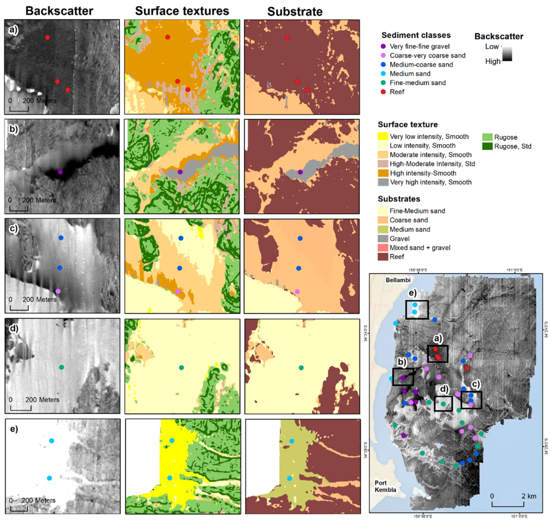
2.6.1. Seabed Textures

Seabed textures represent a classification of the textural components of the seascape which can inform on variability in substrate types where validation data is sparse or absent. Where ground-truthing data is available, substrate classes may be mapped. Examples of seabed texture classifications are provided here for Wollongong and South Solitary Islands. Although ground-truthing sediment data from towed-video could be utilised for South Solitary Islands survey area, for the purposes of this study the area is treated as an area where validation data is not available.
To classify seabed textures, a supervised classification was performed on a multi-band image of backscatter, standard deviation (3-cell radius), and ruggedness (3-cell radius). Backscatter was selected as an input variable due to its relationship with surface composition [69] and ruggedness was selected due to its aforementioned effectiveness at classifying outcropping features. Ruggedness was included in its reclassified form, which simplified the map into rugose and smooth areas, as per the surface elements classification. Standard deviation was, therefore, additionally added to capture finer scale variability in the surface, which may occur over smooth or rugose areas. Backscatter data were first generalised into objects using the mean shift tool in the ArcGIS Segmentation and Classification toolbox prior to generating the composite surface. Standard deviation was reclassified into 15–16 increments (at 0.1 intervals to 1, then intervals of 1 through to 6 for Wollongong, and through to 7 for South Solitary Islands) and ruggedness was reclassified into two increments (break value = 0.0003, in landform classification above). Artefacts were manually edited prior to generation of the composite image.
Representative areas of distinct backscatter intensity and surface complexity were selected as training areas with the Image Classification toolbar in ArcGIS v10.4. For the Wollongong area, the user-defined categories included 8 levels: Very high, high, moderate, low, and very low backscatter intensity over smooth areas; high to moderate intensity with high standard deviation; rugose areas; and rugose areas with high standard deviation. For the South Solitary areas, fewer categories were classified due to the lower variability evident in the backscatter (high, moderate, and low intensity over smooth areas; rugose areas; and rugose areas with high standard deviation). The support vector machine (SVM) classifier was used to classify the multi-band image based on the user-defined classes into a product of surface texture.

2.6.2. Seabed Substrates, Character, and Geomorphology

An example of a substrate classification is provided for Wollongong only, based on the seabed texture classification and sediment grab ground-truthing data. To characterise substrates in the Wollongong survey area, the resultant classified seabed texture layer was overlain with the sediment samples (n = 45) and, where the class consistently represented the associated sediment sample, and the classes were labelled with their associated substrate type. For most sediment grab classes, the sediment class correlated to a distinct seabed texture class. In some instances, a single image class may be associated with multiple substrate types and, in this case, substrate classes were manually separated based on the consistency of backscatter texture and the distinction of class boundaries. For the Wollongong sediment data presented here, the samples described in this study represent a dataset which is more ‘limited’ in detail and coverage, thus constraining the use of statistical mapping approaches such as those presented in the seabed habitat scenario. Detailed sediment analyses will be further explored in separate investigations (see References [70,71]).
The seabed character map aggregates descriptors of the landforms and substrates (or seabed textures) to create a simplified classification of the nature of the surface. A seabed character map is presented for the Wollongong area, created using combined categories from the preceding landform and substrate classifications. A similar seabed character map is presented for the South Solitary Islands, however in this case, where a substrate map was not produced, the seabed character map is instead an integration of the landform and seabed texture classifications. Where formative processes of landform evolution are well understood, this classification may be further developed to classify seabed geomorphology, which incorporates inferences on the processes that shape the landscape. Such is the case for the Wollongong region, where a preliminary geomorphic interpretation is produced.
The seabed character map is modelled from the US Geological Survey California Mapping Program ‘seabed character’ map series, which produces maps classifying seabed slope, backscatter, rugosity, and sediment type [72]. The integration of landform and seabed texture or substrate maps in the present study achieves a similar characterisation of the seabed surface. Landform and seabed texture/substrate layers were integrated together using Union in ArcGIS, and selected categories were carried across to create the character classification. For example, channels and depressions that may be fine, medium, or coarse sands were classified as ‘sandy channels and depressions’. The final categories were chosen to reduce map complexity while also retaining sufficient division of prominent features and textures to suit most users’ requirements. As each map produced is a standalone product, users are able to extract and integrate selected categories from each of the maps. Therefore, although the seabed character map generalises the seabed categories, the detailed divisions are retained within the preceding classifications.
The geomorphic classification, undertaken for the Wollongong case study area, forms the subsequent step to the morphology (landform) classification in Dove et al. [26]. Geomorphic feature terms include reference to feature origin (e.g., abraded platform) and, therefore, further require an understanding of landscape processes for the study area. For example, channel features may be aggregated to ‘paleochannels’. For areas where formative processes are not well understood, the seabed character map may be the final stage of interpretation. For the Wollongong geomorphic interpretations introduced here, the terms applied in this study are based on a limited suite of ground-truthing data, and geomorphic classifications could be refined using a broader suite of sediment characteristics.

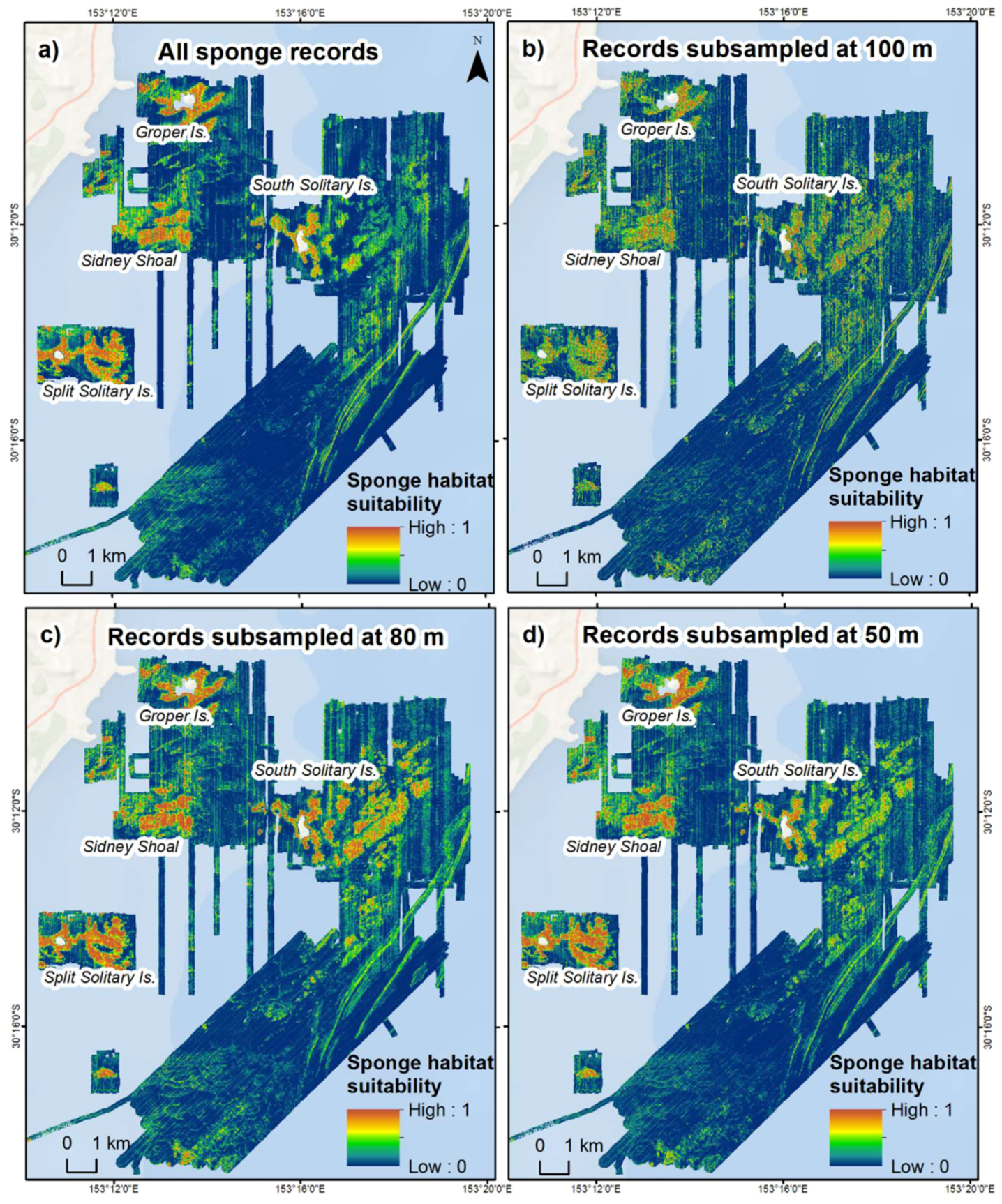
2.6.3. Seabed Habitats

Classified towed underwater video data available for South Solitary Islands were utilised in this study to provide an example of predicted sponge habitat suitability (sample locations shown in Figure 2b). This example illustrates a potential application of habitat suitability modelling using a more comprehensive repository of classified validation data. The towed underwater video data conducted around South Solitary Islands targeted rocky reef habitats and video data were classified for percent cover of benthic organisms and substrates [45], as described in Section 2.3. Sponges were selected as the model target for this study as they were common and well distributed spatially and across depths. Data were modelled in Maxent v3.4.1 software [73] which predicts spatial distributions of species using Maximum Entropy statistical techniques with presence-only data [74,75]. Maxent software was selected due to its widespread use for species distribution modelling and ease of application [76]. Methods were adapted from Linklater [77] which used similar input datasets of towed underwater video, bathymetry, terrain derivatives, and geomorphology to model sponge distributions and other biota in a NSW shelf setting.
Presence-records of sponges were extracted from the classified video dataset. Eight tows, representing approximately 65% of video data, were used for model calibration and the remaining five tows were used for validation. Spatial autocorrelation was explored using the Incremental Spatial Autocorrelation tool in ArcGIS v10.4. Results indicated peak clustering at 180 m, however subsampling at this interval resulted in too few samples to model (11 records for calibration). Data were therefore subsampled at series of increments of 100 m (21 records for calibration), 80 m (27 records for calibration), and 50 m (47 records for calibration), together with all sponge records (362 records for calibration), to explore potential suitable habitat distribution at different subsampling thresholds. To account for geographical sampling bias across the survey area, a 200 m buffer surrounding tow data were used as a bias grid. Maxent modelling were executed using the suite of derived continuous terrain variables described in Section 2.4, with the seabed character classification included as a categorical variable. The inclusion of the seabed character map enables relationships to be explored between prominent landforms and textures with sponge distributions. Maxent modelling was then repeated with the highest-performing variables (ruggedness, backscatter, eastness, broadscale TPI, seabed character) with colinear variables removed.

3. Results

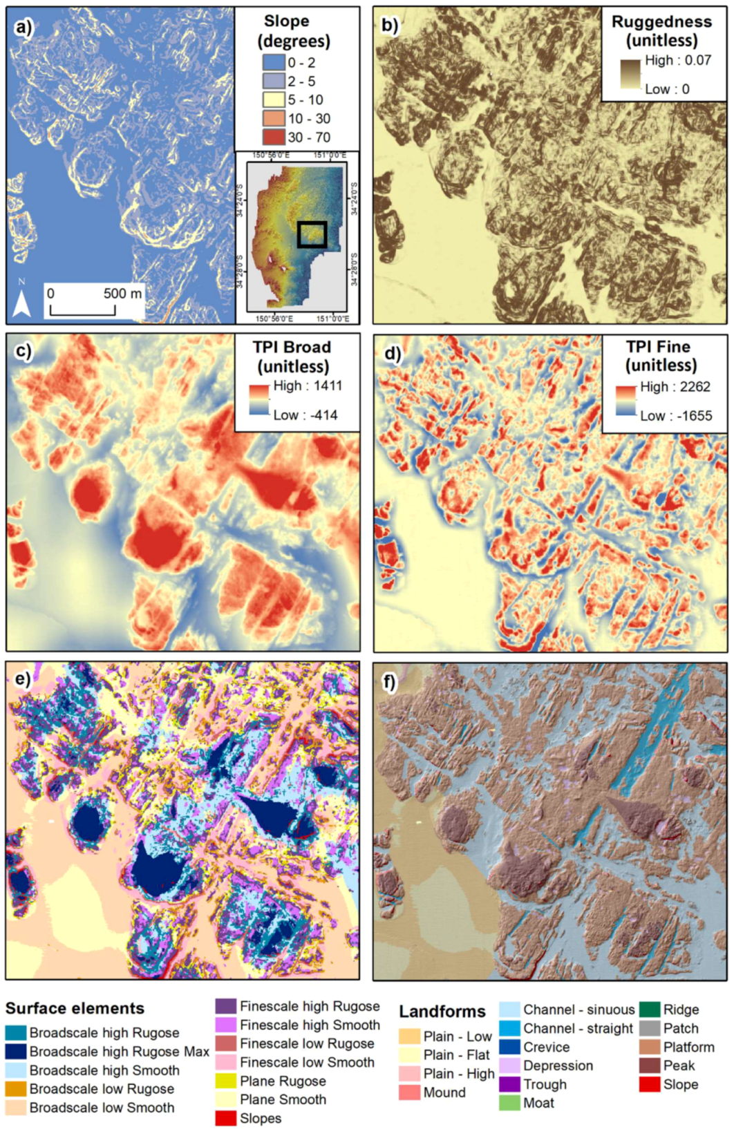
3.1. Terrain Variables

The DEM for the Wollongong area covers 102 km2 in depths ranging 4 to 62 m water depth. The majority of MBES mapping (84%) occurred in 25 to 55 m depth, with shallower depths aimed to be targeted with marine LiDAR [59]. The DEM for the selected area surrounding South Solitary Islands covers 137 km2 in depths ranging 2 to 83 m water depth. The terrain variables determined to be most suitable for feature delineation around Wollongong include slope (Figure 4a), ruggedness (Figure 4b), broadscale TPI (150-cell radius) (Figure 4c), and finescale TPI (27-cell radius) (Figure 4d). These selected terrain variables were input into the classification dictionary to classify surface elements (Figure 4e) and landforms (Figure 4f).

3.2. Seabed Morphology

3.2.1. Surface Elements
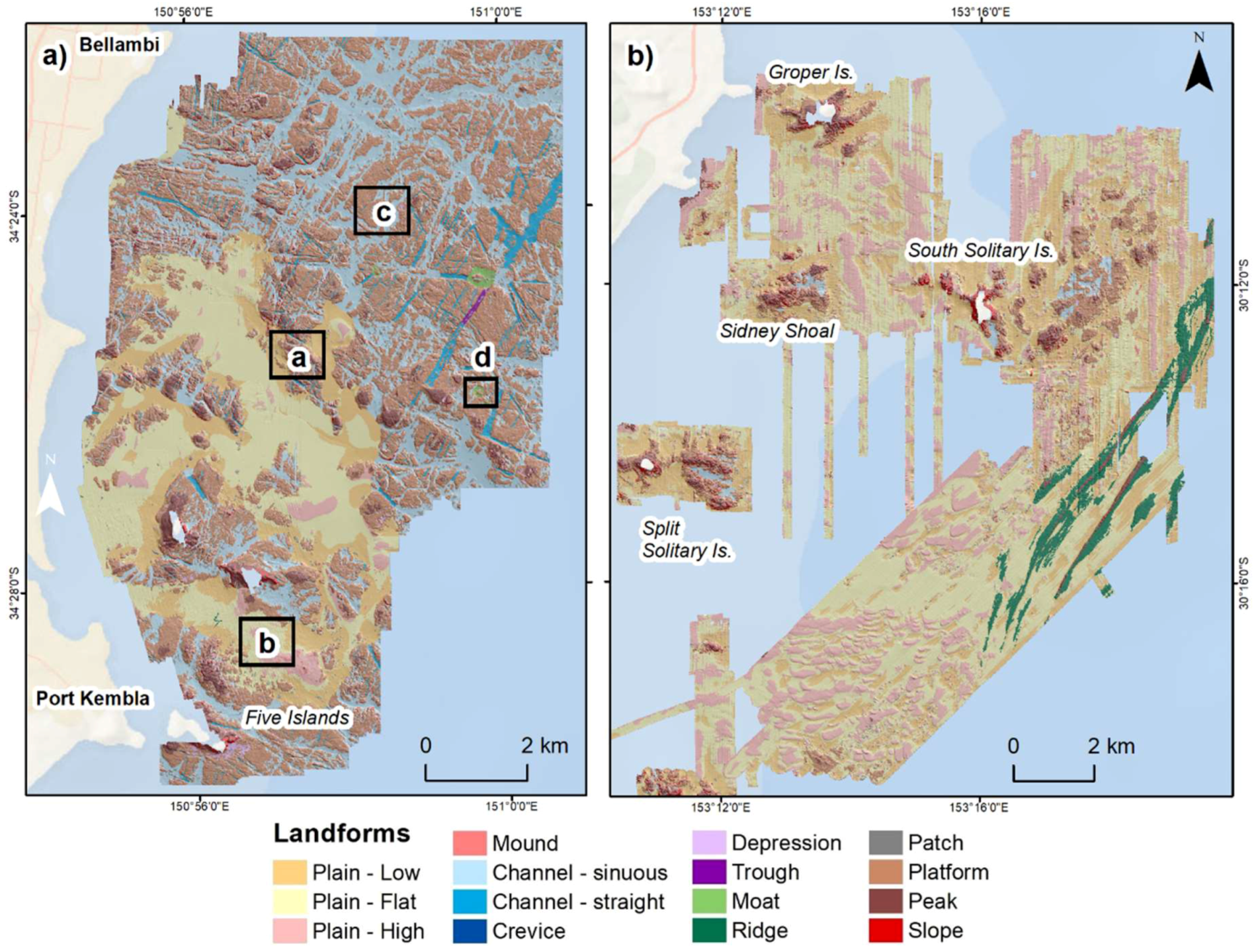
As can be seen from Figure 4e, the surface elements classification segmented the surface into a range of morphological units characterising surface roughness and relative position which effectively delineated the boundaries of features, subsequently edited to landforms (Figure 4f). It can be seen in this example that the platform features are comprised of a mix of rugose and smooth components, which is typical of this low-profile reef feature; and sinuous and straight channels which intersect the platform outcrops are primarily comprised of broadscale and finescale lows and planes. Due to the number of categories generated in the surface elements classification, it is beneficial to summarise this surface into generalised categories (as described in Section 2.5.3) prior to editing into landforms. An example of these summarised surface elements is presented in Figure 5.
The rugose components of the surface elements classification were compared to the previously digitised ‘reef’ and ‘non-reef’ layer for a selected area of the South Solitary Islands dataset, which was selected as a representative area of existing data from the OEH repository (Figure 5). Quantitative comparisons were undertaken to compare the area of digitised reef within the area of interest shown in Figure 5 (1.9 km2) to the collective area of rugose outcrop, peak, and slope elements (2.7 km2). When overlaying the coverages of the two methods, 66% of classified reef extent were captured by both the semi-automated (rugose outcrops, peaks, slopes) and manual (digitised reef) methods. The semi-automated approach captured 31% of additional reef which was not captured by the digitised approach, and only 3% of additional reef was captured by the digitised-only method. The ruggedness threshold used within the surface elements classification captured additional areas of rugose surfaces around the outcrop edge which were not captured by the digitised reef extent. This is, in part, due to the 3-cell window radius of the ruggedness variable and, in part, due to the orientation of hillshade used during manual digitisation which may bias boundary interpretation [78]. Artefact areas were also additionally captured as rugose outcrops which inflated the area calculation. While the automated approach captured a greater area of potential reef, visual assessment of the two methods shows the spatial extent of reef identified during manual digitisation was effectively captured by the surface elements classification.
The effectiveness of the surface elements classification depends on the level of artefacts present within a survey area. This particularly relates to the ruggedness variable which is sensitive to artefacts (see Appendix A, Figure A1). Interrogation of TVU surfaces shows poorer uncertainty values associated with the older South Solitary Islands survey area relative to the newest Wollongong survey area (Figure 6), associated with the applications of different sonar technologies and improvements to vessel motion correction solutions. Areas of greater uncertainty are associated with track-line artefacts (e.g., at nadir), noise on the end-beams, motion system errors, and roll artefacts. These variations in the surface can incorrectly appear as areas of higher surface complexity, which are, in turn, captured within the classification as rugose surfaces. A comparison of summarised surface element categories (Figure 6e,f) highlights the challenges of applying the surface elements classification to data which may contain such artefacts.

3.2.2. Landforms

The landform classification method developed for the Wollongong pilot area (Figure 7a) was applied to the South Solitary Islands study area (Figure 7b). The classification dictionary effectively captured surface element boundaries and the features were edited into landforms using the drainage surface for reference.
Similar landform features were mapped across South Solitary Islands and Wollongong, with differences in the spatial extent of each landform. The Wollongong area possess a greater proportion of platform reefs (Figure 8a), which comprise 43% of the mapped area. Plains intersect platform outcrops occurring as predominately flat plains (15% of the mapped area). By contrast, platform and patch reefs comprise a smaller relative proportion of the mapped area (9%) around the South Solitary Islands, and flat plains are the dominant landform type (37%). Platform outcrops occur in greatest extent around the offshore islands of South Solitary Island, Split Solitary Island, Groper Islet, and Sidney Shoal, with smaller patch reefs scattered across the case study area. Broad plains are ubiquitous across the survey area (83%) and exhibit a mixture of high, low, and flat morphologies. The more restricted plains in the Wollongong area (comprising 25% of the mapped area) also possess complex morphologies, with low plains often adjacent to platform outcrops and few high plain areas (Figure 8b).
Between and within the platform outcrops in Wollongong, a diverse range of smooth features were mapped including straight and sinuous channels, troughs, crevices, depressions, and moats (Figure 8c,d). Interconnected channels form an extensive network across the platform surface, occurring in greatest prevalence as sinuous channels (22% of the mapped area). Flow pathways of the channel networks generally travelled in an easterly direction, as highlighted by the surface drainage grid. Channels, depressions, and other low elements were less prevalent around South Solitary Islands due to the more restricted extent of platform outcrops.
Characteristics unique to the Wollongong landform classification were circular moat features which were documented across the southeastern Wollongong survey area in 38 to 54 m depth (Figure 8d). These features range from 100 to 550 m in width and are characteristically exhibited a circular depression with a central rise. Such features were not documented around the South Solitary Islands survey area and have not been identified within prior surveys. Expansive ridge landforms were a distinguishing feature of the South Solitary Islands area, mapped at 60–80 m depth in the southeastern survey area and totaling 5.2 km2 (Figure 7b). These features extend 10 km and form as a series of shore-parallel ridges spaced up to 500 m apart. Comparatively, only one outcrop of small ridge features (less than 200 m in length) were mapped around Wollongong and did not occur in a shore-parallel formation.
Overall, the classification methodology developed for the newest area of MBES data at Wollongong was effectively applied to the older area of existing MBES data offshore of Solitary Islands. However, the increased noise associated with the older survey data resulted in a higher number of artefacts which required a greater time investment to manually edit the landform classification.

3.3. Seabed Composition

3.3.1. Seabed Textures

Backscatter data for the Wollongong case study area indicated extensive areas of high to moderate backscatter intensity (Figure 2a). The surface texture classification performed for the Wollongong case study area identified extensive rugose areas, which were typically high-to-moderate backscatter intensity (Figure 9a). Low-to-moderate backscatter intensity areas dominated the plain areas between the rugose outcrops. The plain areas were the focus of sediment grab sampling (Figure 2a and Figure 9b), to identify the source of prominent variability in the backscatter signal, despite the relatively smooth bathymetry.

3.3.2. Seabed Substrates, Character, and Geomorphology

Correlation between the sediment types surmised from the grab samples and the supervised classification of surface textures enabled a substrate classification map to be produced (Figure 9b). The substrate map shows that the plain areas are variably comprised of fine and coarse sand facies, which are irregularly distributed between rocky reef outcrops that are associated with areas of higher ruggedness and standard deviation. Coarse sands represent the most dominant soft-substrate class (25% of the mapped area), comprising the majority of the channel and depression areas, and a subordinate proportion of plain areas. Fine sands, identified by consistently low backscatter intensity, are the second most dominant substrate type (8% of the mapped area) and comprise the majority of plain areas. Gravels are associated with very high backscatter reflectance and occur in restricted areas of bathymetric lows of the plain. Several grabs retrieved from the Wollongong compartment recovered benthic reef fauna and negligible sediment and were classified as rocky reef.
Seabed character classifications were undertaken for the Wollongong area using the landform and substrate maps (Figure 9a–c and Figure 10), and for the South Solitary Islands area using the landform and seabed texture maps (Figure 11a,b). The seabed character map for the Wollongong area was further developed into a geomorphic map (Figure 9d), informed by an understanding of the sedimentary environment and regional geology sourced from the substrate classification and existing literature. While geomorphic features were not mapped around the South Solitary Islands, similar processes can be inferred due to its similar inner- to mid-shelf setting on the NSW passive continental margin.
Platform, peak, and slope landforms comprise a mix of high- to low-intensity backscatter areas as the reef outcrops can vary from exposed reef outcrops to reefs with sediment veneers or colonised by benthos. These landforms were aggregated to abraded platforms for the geomorphic interpretation, which form the majority (66%) of the mapped survey area offshore of Wollongong. Plain areas appeared to comprise a fine-sediment sand sheet overlying coarser sediment deposits as described above, with gravel beds present at the base of scour depressions. Channels which dissect the reef platforms were interpreted as paleochannels, with straight-walled channels and troughs likely associated with structural displacement of the bedrock geology (e.g., faults or joints). Crater features, which represent moat landforms, scattered in the eastern survey area were enigmatic features not currently documented elsewhere on the NSW seabed.
The seabed character classification for the South Solitary Islands area indicates the area is dominated by low-intensity plains (60% of mapped area), which are inferred to be comprised of sandy substrates, similar to the medium-to-fine sands observed around Wollongong. Lenses of high- to moderate-intensity textures occur as lenses within the plain, which are likely comprised of coarser sands and gravels, as observed in the scour depressions around Wollongong. Platform and patch reefs with slopes and peaks (18% of mapped area, collectively) are observed around the islands and shoals of South Solitary Island, Groper Island, Sidney Shoal, and Split Solitary Island. These represent a significantly lower proportion than were observed around Wollongong. The South Solitary Islands area also has a lower proportion of channels and depressions (1% of mapped area), which correlates to the reduced extent of outcropping reef. Of the channels and depressions mapped between the reef outcrops, they are primarily comprised of high- to moderate-intensity textures, indicating coarser-grained materials such as coarser sands, gravels, and cobbles. Expansive ridges are a characteristic feature of the South Solitary Islands area, as described in Section 3.2.2 (5% of mapped area, excluding peaks). These landforms are comprised of primarily low-intensity textures, with high- to moderate-intensity smooth and rugose textures on the upper areas of the ridge feature, with peaks defining the uppermost ridge crest.

3.3.3. Seabed Habitats

Predictive mapping of suitable sponge habitat was performed for the South Solitary Islands case study area in Maxent software using input ground-truthing data together with continuous terrain variables and the categorical seabed character variable. Modeling was performed at a range of subsampling intervals to account for spatial autocorrelation within transect data. Comparisons of model outputs at the subsample thresholds tested are provided in Appendix C, Figure A2. The modelled distribution of sponge habitat indicated consistent patterns across all subsample thresholds, with sponges predicted in areas of outcropping reef across all depths. Backscatter, ruggedness, bathymetry, seabed character, eastness, and broadscale TPI were the top explanatory variables across all models, with colinear variables removed. Suitable habitat areas are presented for all sponge records with top-performing continuous variables (Figure 11c) and with the addition of the seabed character categorical variable (Figure 11d). Sponge occurrence was predicted as highest on the reef outcrops surrounding South Solitary Island, Groper Islet, and Sidney Shoal. Areas of predicted sponge habitat were also associated with high backscatter intensity plain areas, which may represent unconsolidated hard substrates such as cobbles.
Contributions of top explanatory variables differed between subsample distance thresholds, with backscatter appearing as the top permutation contributor for all data and 50 m subsampled data, and ruggedness the top permutation contributor for 80 m and 100 m subsampled data. While the variation in contributions of explanatory variables is not a concern for the purposes of this study, these results highlight the influence of the number and distribution of samples on model performance. All models had similar area under curve (AUC) values, ranging 0.93 (80 m subsample) to 0.95 (100 m subsample). The addition of seabed character resulted in predicted surface of AUC = 94.0, with seabed character identified as the third highest permutation contribution (16%) to the predicted output, following backscatter (38%) and bathymetry (29%). Sponge occurrences appeared to be most associated with rugose ridges, low-intensity ridges, and high- to moderate-intensity channel and depression features, with weakest associations to low-intensity plains. As the seabed character map was generated using a number of the selected input variables, these results may be correlated, and therefore the contribution of seabed character alone was explored. These results showed the strongest association of sponge occurrence to features (decreasing from highest): peaks, slopes, high- to moderate-intensity channels and depressions and rugose ridges; with weakest associations to low-intensity plains.

4. Discussion

Here we present a comprehensive and flexible classification framework for high-resolution seabed data for a continental shelf environment which aligns to national and international nomenclature. The methodologies and techniques presented here, developed from a 5-m MBES DEM, can be applied to the statewide marine LiDAR program currently being undertaken in NSW, as part of SeaBed NSW, and integrated with new and existing MBES data to produce a seamless classification for nearshore and offshore seabed environments.

4.1. Seabed Morphology

Semi-automated procedures were developed for the classification of seabed morphology, which includes techniques for classifying surface elements, theoretical surface drainage, and landforms. The classification approach of morphological units conforms to the definitions of landforms in Evans et al. [18] and morphology in Dove et al. [40]. The implementation of the landform framework developed for the Wollongong pilot area was shown to be effectively applied to a selected area within the existing data repository at South Solitary Islands using the same terrain variables and classification dictionary schema. The application of the landform classification method to the older South Solitary Islands dataset captured comparable surface element and landform features, thus demonstrating the transferability of the method to other existing datasets held by OEH and to comparable survey areas elsewhere.
The generation of the surface elements map effectively delineated the boundaries of prominent features within the area of interest which subsequently formed the boundaries of the mapped landforms. Adopting a semi-automated approach for the surface elements classification significantly reduced the time taken for the user to manually digitise feature boundaries and resulted in standardised output product. The spatial extent of rugose outcrop elements was shown to capture similar extents to those manually digitised and resulted in reduced subjectivity. Furthermore, the range of categories captured within the surface elements classification produces a more comprehensive suite of surface components compared to the singular measure of digitised reef extent, which better reflects the variability in surface shape and complexity. As this classification of rugose areas approximates outcropping reef extent, it can be integrated into the OEH statewide habitat map [50] which includes reef areas digitised from MBES data, marine LiDAR data, sidescan sonar data, and aerial imagery.
The subsequent classification stages to define landforms required greater user input via manual digitising. However, user input at this stage of mapping interpretation is considered important to incorporate expert knowledge of feature identification [17], which includes viewing the landforms within the context of the surrounding seascape and ensuring the features identified match the landform definitions (which may include feature descriptions that are challenging to automate). While the techniques of classifying surface elements and landforms were effectively transferred to older datasets, the efficiency decreases as noise increases and therefore the suitability of applying this method needs to be assessed on a case-by-case basis (see Figure 6). The generation of the TVU surface can assist in accounting for noisier areas within surveys and may be utilised to identify areas for further review when editing the surface elements to the landform stage.
As outlined in this study, the ruggedness threshold value may be increased in cases where greater artefacts are apparent. In these cases, greater manual editing is required as an increased proportion of the outcropping surface, which would otherwise be classified as rugose outcrops at a lower threshold, is classified as smooth outcrops. For areas of cleaner bathymetry data, it is recommended to lower the ruggedness threshold beyond that which was applied in this study, as is discussed in Appendix A. Threshold parameters for slope and TPI variables in the BTM classification may also be adjusted to capture features of interest as relevant to other study areas. However, the classification dictionary presented in this study should be effective for applications to similar environments in areas of similar data quality (as shown in the TVU maps in Figure 6), with re-parameterisation of the ruggedness value as required.
The classification of seabed morphology presented in this study is relevant to the map scale of the data utilised (5-m cell size, map scale approximately 1:5000). Features classified at this scale may present differently when viewed at coarser or finer scales. For example, features that may be identified as plains in the current landform classification may be classified as channels at a coarser map scale, when they are viewed in context with their connection to the surrounding onshore catchment area. Channels and depressions within the platform reef identified in the current Wollongong survey area classification, for example, may not be visible at the broader spatial scales, either due to lower resolution generalising the surface or the detail of such features may be impracticable to map at broader scales.
Furthermore, the new method of morphology classification presented in this study delineates feature boundaries across the entire seascape in one complete stage during the process of classifying surface elements. This results in features with boundaries that are not overlapping, and, as such, this classification may not be suitable for applications where overlapping features are desired (e.g., Reference [29]). Alternative classification methods may apply customised methodologies to identify and classify individual landform features, which may be in turn integrated into a complete map (e.g., References [28,29]). Due to the extensive coverage of new and existing seabed data held by OEH, and the need to generate a broad suite of data products, it was desired to generate a complete classification of the seascape in a simple and transferable workflow. The simplicity of the method presented, and the accessibility of the software and tools used to perform the classifications, was desired for ease of application and repeatability over time.
Overall, the methodologies for seabed morphology classifications described in this study were successfully applied to data in the 0 to 85 m depth range and were demonstrated to be effective for classification of features in this shelf zone. The methods presented can be applied to existing and future MBES and marine LiDAR data collected under SeaBed NSW and future programs and can be applied to comparable shelf environments. The methodologies presented will continue to be expanded and developed to account for terrestrial data and features not accounted for by this study, such as submerged artificial structures.

4.2. Seabed Composition

Selected examples of substrate and habitat classifications were provided to exemplify alternate approaches for seabed classifications to suit common seabed sampling scenarios where validation data is absent, limited, or comprehensive. The classifications of seabed composition products presented in this study are intended as illustrations of the types of map products that can be produced, and, more importantly, how the products inter-relate with the other seabed products outlined in the proposed classification framework.

4.2.1. Wollongong Case Study Area

For the Wollongong case study area, example maps were produced of seabed texture, substrate, seabed character, and geomorphology which utilised sediment grab samples analysed to broad grainsize classes only, representing a scenario with limited validation data. The substrate classification produced for the Wollongong area (Figure 9b and Figure 10) was derived from the backscatter data, surface texture analysis, and the ground-truthing results from sediment grab sampling. The resultant map depicts a highly complex inner-continental shelf seabed substrate that is dominated by relatively planar rocky reefs of variable roughness, which are interspersed with predominantly sandy sediments that form irregular plains in bathymetric lows. The sediment types retrieved in grab samples generally reflect the existing models for this region [65,66,79], although their distributions across and along the seabed are highly irregular, most likely due to the dominance of the rocky reef structures and the effects of complex hydrodynamics imposed by the islands and reefs.
The medium sand class sampled in the shallowest plain areas reflects the nearshore or ‘shoreface’ sand facies [65], which are clean, moderate-to-well sorted, and fine-to-medium sand, that is predominantly composed of reworked and often iron-stained quartz grains with a secondary carbonate component. In the Wollongong area, that sand class is restricted to the shallowest plain areas mapped, which remain connected to the modern beach systems onshore. Elsewhere, the dominance of rocky reefs likely interrupts the seaward extent of that sediment class.
The fine and coarse sand classes that comprise the majority of the sandy plains in the Wollongong study area reflect the inner-shelf sand sheet facies [65,79], which usually forms a coast-parallel deposit between 20 to 60 m water depth along parts of the inner shelf that feature more regular bathymetry. The sand sheet is often characterised by an irregular distribution of fine-to-coarse quartz sand, which is thought to have derived from repeated (and often ongoing) in situ marine reworking of the same palimpsest parent material. As such, the fine and coarse sand classes identified here are likely related, the former representing the aggregation of finer material that is intermittently mobilised by strong waves and currents.
Variability in the backscatter intensity associated with the coarse sand class (Figure 9a,b) likely reflects varying carbonate content with proximity to rocky reefs. For example, Lean and Peat [64] identified two classes of coarse ‘grit’ in this region, which they differentiated based on the relative proportion of reworked carbonate material. The gravel class likely reflects localised scouring around emergent rocky reefs, where only the coarsest sediments from the parent material and local carbonate production can withstand enhanced bottom currents. The results of sedimentology and mineralogy analyses of the sediment grab samples that are being pursued in collaboration with the University of Wollongong are expected to reveal further insights on the nature and complexity of sedimentary substrates within the region.
Interpretations of the sedimentology and regional geology as discussed above informed the interpretation of geomorphology. A diverse range of geomorphic features were mapped within the Wollongong survey area, associated with an array of landform types. The extensive reef platforms are inferred to represent abraded late Permian Shoalhaven Group and Gerringong Volcanic bedrock sequences (composed primarily of sandstones, siltstones, and latite members), with identification based on outcropping geology onshore and stratigraphic cross sections [80]. These bedrock platforms likely form part of the East Australian Marine Abrasion Surface, which has been mapped off the Sydney coast to the north [81]. The abraded platform is inferred to result from wave action eroding and planating the bedrock outcrops over multiple sea level cycles throughout the Paleozoic to Mesozoic.
The channel and trough features dissecting the platform were likely active fluvial systems during periods of lower sea level, with scouring and sediment deposition occurring during cycles of shelf inundation and exposure. Plain areas are comprised by fine-to-coarse sand sheets which correlate to the inner shelf sand sheet described by Roy et al. [79], which is dominated by heavily reworked palimpsest sands, as discussed above.
Enigmatic crater features were observed for the first time in the Wollongong survey area and such features may originate from volcanic processes or impact sources. These are most likely volcanic maar-diatreme features [82] which have been documented in terrestrial landscapes in the Illawarra and Sydney regions [83]. Branagan [84] suggests there are possibly 150 terrestrial diatremes in the Sydney Basin, which relate to volcanic activity that probably occurred sporadically from Middle Triassic to early Jurassic time. Crawford et al. [85] indicates that these features are essentially the cores of eroded maars, some of which may have erupted a number of times. The terrestrial diatremes in the Sydney region exhibit downward-tapered carrot-shaped cores surrounded by sedimentary rock (sandstones and siltstones). The cores are typically made up of breccia, sedimentary breccia, and basalt interpreted to be volcanic collapse structures formed following eruptions resulting from the mixing of hot magma and water. Most of these features weather easily and thus appear as circular depressions in the landscape [79]. Terrestrial and submarine examples of impact craters with similar morphologies have also been documented in Australia and internationally (e.g., References [86,87,88]). The origin of these crater features cannot be ascertained definitively from morphology alone, and further research would be needed to determine formative processes.

4.2.2. South Solitary Islands Case Study Area

The seabed character map generated for the South Solitary Islands area provides an example of a classification which can be produced where validation data is absent, such is the case for many MBES and marine LiDAR survey areas along the NSW coast. Substrate types can be inferred based on results from comparable study areas and data from the existing literature. In the South Solitary Islands area, vast sandy plains were inferred across the majority of the seascape, with coarser lenses of gravel or cobbles and bedrock rocky reefs surrounding islands, islets, and shoals. Sediment sampling conducted around the Solitary Islands has recovered gravel material from the high-to-moderate backscatter intensity lenses, and fish assemblages around these soft-sediment environments have been shown to be distinct from the assemblages observed in rocky reef environments [89]. The role of these higher-intensity soft-sediment areas as important habitat for organisms such as sponges is supported by our study, where sponge occurrences were shown to correlate with areas of high to moderate intensity in channels and depressions, and to a lesser extent in plain areas.
In addition to the high- to moderate-intensity channels and depressions, the seabed character types which appeared most relevant to sponge occurrence included peak, slope, and ridge landforms. Backscatter, bathymetry, ruggedness, and seabed character were identified as the strongest performing variables explaining sponge occurrence in our study. The inclusion of seabed character as an important explanatory variable supports the findings of a similar study undertaken around the NSW island shelves of Lord Howe Island and Balls Pyramid, which identified geomorphology as an important explanatory variable which improved predicted species distributions [77].
While a geomorphic classification was not undertaken for the South Solitary Islands survey area, similar geomorphic features are inferred. Platform and patch reef outcrops likely comprise exposed bedrock reefs, overlain by sand sheets deposited during the last glacial transgression [79]. Expansive ridges were documented in the deeper waters of the survey area in 60 to 80 m depth, which are inferred as paleo-shoreline features likely comprised of remnant barrier deposits, such as those documented elsewhere along the Australian continental shelf in similar depths [45,90,91]. Similar paleo-shoreline features have been mapped around the mid-oceanic Lord Howe Island and Balls Pyramid shelves, and are interpreted as potential drowned coral reefs, due to the known accretion of coral reefs around the island shelves in the Holocene and present-day [92,93,94]. While coral growth occurs in the South Solitary Islands area, reef-forming accretion is not documented and the rocky reefs documented to date comprise bedrock outcrops [95,96]. It, therefore, appears the ridges in the South Solitary Islands area most likely comprise drowned coastal sand barrier deposits that formed at times of lower sea level during the late-Quaternary glaciations [90,91].
The map of predicted sponge habitat presented in this study is intended to provide an illustration of how habitat classifications fit within the proposed classification framework and how the biotic data can be integrated with other compositional or morphological map products. Individual maps of species distributions, such as the example of predicted sponge occurrence in the present study, may be amalgamated into categorical maps of benthic communities or biotopes (e.g., Reference [23]). Similar predictive modelling approaches may also be applied to generate surfaces of sediment properties (e.g., Reference [97]) or benthic diversity metrics (e.g., Reference [10]). While detailed analyses of the predictive modelling were outside the scope of this study, our results highlighted common challenges of predictive mapping in marine environments including accounting for spatial autocorrelation in subsampling design [98]. Our findings showed the towed underwater video data exhibited spatial autocorrelation within the subsampling intervals tested, however the detection of spatial autocorrelation in this case was balanced with the need to maintain a viable calibration and validation dataset. Our results of predicted sponge habitat at varied subsample intervals indicated consistency in the predicted spatial distribution of sponges, with slight variations in the order of selected top explanatory variables. For future applications of the towed underwater video data, appropriate subsampling intervals should be further tested and explored.

4.3. Applications for Coastal and Marine Management

The detailed information on seabed shape and composition presented in this study provides fundamental baseline data which are critical to localised assessments of coastal risk. Detailed bathymetry is a necessary input into any modelling of coastal hazards like storm surge, waves, and tsunamis, while understanding the composition and distribution of substrates enables more reliable sediment budget analysis, reducing uncertainty in erosion risk modelling (e.g., Reference [12]). Substrate mapping also provides insights into sediment dynamics within each region, which can inform sediment compartment boundary identification and estimation of sediment transport rates between key depositional features (e.g., References [70,99]).
Substrate, landform, and geomorphic maps can be utilised as surrogates to infer the distribution of biological communities where sparse ground-truthing data exists [6]. In NSW, substrate classes have been shown to support distinct pelagic communities in soft-sediment areas [89] and gradients of terrain variables and geomorphic features have shown to relate to patterns in the distribution and abundance of benthic and pelagic communities [4,62]. The findings of the present study provide evidence in further support of the role of continuous variables, such as bathymetry, backscatter, and ruggedness, and categorical variables, such as seabed character, in explaining the predicted spatial distributions of sponge communities. The demonstrated importance of seascape metrics and categorical maps, such as seabed character and geomorphology, highlights the need to generate more informative maps of seabed morphology and composition, beyond the previous classification of reef and soft-sediment extent, to adequately capture benthic and pelagic variability across the seascape.
Geomorphic and landform classifications furthermore quantify the geodiversity present within a region. Geodiversity is the range of geological features present within a landscape or seascape [100]. The need to document and recognise geodiversity with a seascape is an area of growing attention [101], and the identification of features in the Wollongong compartment contributes to our local and global understanding of submarine geodiversity. The craters mapped in the Wollongong compartment emphasise the importance of recognising geodiversity as few studies globally have documented crater features in submarine environments (e.g., References [86,87]). Discovering these previously hidden features highlights the critical need to collect baseline maps of the seabed, which are the fundamental first step in managing a coastal and marine environment.

5. Conclusions

This study presents a methodological framework and new techniques for classifying seabed morphology and composition on continental shelf environments, exemplified with case study areas along the subtropical-temperate passive continental shelf of NSW, Australia. The methodology presented in this study significantly extends upon historical classification systems applied to seabed data in NSW and generates a comprehensive product suite which conforms to national and international standards.
The key outcomes of this study include:
  • Development of a new semi-automated method for classifying seabed landforms which provides an informative product of seabed morphology;
  • Presentation of example methodologies for substrate and habitat classifications which vary depending on the availability and characteristics of ground-truthing data;
  • Integration of landform and substrate classifications to produce seabed character and geomorphology maps which generalise the nature of the seabed, with inferences on feature origin where appropriate;
  • Creation of a consistent methodology which can be effectively applied to new MBES and marine LiDAR data, in addition to the repository of bathymetric data collected by OEH and comparable survey areas elsewhere. The method described is suitable for 5-m DEMs as inputs, and the framework is scalable to finer or coarser resolution data as needed.

Supplementary Materials

Bathymetric data utilised in this study are available online from the Australian Oceanographic Data Network: https://portal.aodn.org.au/.

Author Contributions

Conceptualization, M.L.; methodology, M.L.; data acquisition, T.C.I., B.D.M., M.A.K., and M.D.S.; MBES data processing, K.M.A., T.C.I., and B.D.M.; formal analysis, M.L.; writing—original draft preparation, M.L.; writing—review and editing, M.L., T.C.I., M.A.K., D.J.H., B.D.M., K.M.A., and M.D.S.; project administration, D.J.H.; funding acquisition, D.J.H.

Funding

This research was funded by NSW Climate Change Fund through the Coastal Management Funding Package.

Acknowledgments

We gratefully acknowledge vessel captain Jeff Miller for his significant contribution to the SeaBed NSW program. Thank you to: Joseph Neilson for classifying HabMap video data at South Solitary Islands and contributing to data collection; Alan Jordan, Edwina Foulsham and Peter Davies for their contributions to the collection and processing of survey data under the HabMap program; and Geoscience Australia for use of sediment grab sampling equipment. Thanks also to Martin Fitzhenry (OEH) for his peer-review of the manuscript and to the two reviewers who provided valuable feedback which greatly improved the manuscript.

Conflicts of Interest

The authors declare no conflict of interest.

Appendix A

Figure A1. Comparison of ruggedness (VRM) thresholds, calculated with Benthic Terrain Modeler v3 extension to ArcGIS: (a) Ruggedness reclassified at 0.00003; and (b) ruggedness reclassified at 0.0003. The higher threshold of 0.0003 was utilised in the classification dictionary presented within this study to minimise manual editing of artefacts, however lower thresholds are recommended where possible to capture a greater extent of outcropping rugose reef features.
Geosciences 09 00141 g0a1

Appendix B

Table A1. Definition and sources of landform feature terms used in this study.
TermDefinitionSource
ChannelA linear or sinuous depression on an otherwise flat surface[42]
CreviceA narrow opening or fissure, especially in a rock or wallTerm in [40], definition from Oxford Dictionary 2018
DepressionA low-lying area surrounded by higher ground and with no outlet or opening (i.e., closed)[42]
MoatAn annular depression that may or may not be continuous, located at the base of many seamounts or islands[37]
MoundA low, rounded natural hill of unspecified origin, which is generally less than 3 metres high and composed of earthy material[39]
PatchIndividual outcrops with circular or oblong shapes and vertical reliefs of one meter or more in relation to the surrounding seafloor. These outcrops are isolated from other outcrop featuresTerm in [40], modified from ‘Patch coral reef’ definition in [39]
PeakA conical or pointed elevation at the summit of a larger feature.[37]
PlainAny land with a flat or very slightly undulating surface. A flat, gently sloping or nearly level region of the seafloor[38]
PlatformAn elevated, level, or nearly level surface bound by a descending slope on all sides.[42]
Term (cont’d)Definition (cont’d)Source (cont’d)
RidgeA long, narrow elevation, usually sharp crested with steep sides. Larger ridges can form an extended upland between valleys[42]
SlopeAn inclined surface or line. The degree of inclination to the horizontal. Usually expressed as a ratio[38]
TroughA long depression generally wide and flat bottomed with symmetrical and parallel sides[37]

Appendix C

Figure A2. Raw output from Maxent modelling at varied subsample threshold distances to account for spatial autocorrelation including: (a) All data records; and records sampled at (b) 100-m, (c) 80-m, and (d) 50-m distance thresholds. Subsampled data were determined to have too few records for modelling, and, therefore, results utilising all data records were presented.
Geosciences 09 00141 g0a2

References

  1. Brown, C.J.; Sameoto, J.A.; Smith, S.J. Multiple methods, maps, and management applications: Purpose made seafloor maps in support of ocean management. J. Sea Res. 2012, 72, 1–13. [Google Scholar] [CrossRef]
  2. Cogan, C.B.; Todd, B.J.; Lawton, P.; Noji, T.T. The role of marine habitat mapping in ecosystem-based management. ICES J. Mar. Sci. 2009, 66, 2033–2042. [Google Scholar] [CrossRef]
  3. McArthur, M.A.; Brooke, B.P.; Przeslawski, R.; Ryan, D.A.; Lucieer, V.L.; Nichol, S.L.; McCallum, A.W.; Mellin, C.; Cresswell, I.D.; Radke, L.C. On the use of abiotic surrogates to describe marine benthic biodiversity. Estuar. Coast. Shelf Sci. 2010, 88, 21–32. [Google Scholar] [CrossRef]
  4. Rees, M.J.; Knott, N.A.; Neilson, J.; Linklater, M.; Osterloh, I.; Jordan, A.; Davis, A.R. Accounting for habitat structural complexity improves the assessment of performance in no-take marine reserves. Biol. Conserv. 2018, 224, 100–110. [Google Scholar] [CrossRef]
  5. Huang, Z.; Brooke, B.P.; Harris, P.T. A new approach to mapping marine benthic habitats using physical environmental data. Cont. Shelf Res. 2011, 31, S4–S16. [Google Scholar] [CrossRef]
  6. Harris, P.T.; Baker, E.K. Seafloor Geomorphology as Benthic Habitat: GeoHAB Atlas of Seafloor Geomorphic Features and Benthic Habitats; Elsevier Science: Burlington, NJ, USA, 2012; p. 947. [Google Scholar]
  7. Andersen, J.H.; Manca, E.; Agnesi, S.; Al-Hamdani, Z.; Lillis, H.; Mo, G.; Populus, J.; Reker, J.; Tunesi, L.; Vasquez, M. European broad-scale seabed habitat maps support implementation of ecosystem-based management. Open J. Ecol. 2018, 8, 86–103. [Google Scholar] [CrossRef]
  8. Harris, P.T.; Whiteway, T. High seas marine protected areas: Benthic environmental conservation priorities from a GIS analysis of global ocean biophysical data. Ocean Coast. Manag. 2009, 52, 22–38. [Google Scholar] [CrossRef]
  9. Moore, C.; Drazen, J.C.; Radford, B.T.; Kelley, C.; Newman, S.J. Improving essential fish habitat designation to support sustainable ecosystem-based fisheries management. Mar. Policy 2016, 69, 32–41. [Google Scholar] [CrossRef]
  10. Huang, Z.; McArthur, M.; Przeslawski, R.; Siwabessy, J.; Nichol, S.; Brooke, B. Predictive mapping of soft-bottom benthic biodiversity using a surrogacy approach. Mar. Freshw. Res. 2014, 65, 409–424. [Google Scholar] [CrossRef]
  11. Hanslow, D.J.; Dela-Cruz, J.; Morris, B.D.; Kinsela, M.A.; Foulsham, E.; Linklater, M.; Pritchard, T.R. Regional scale coastal mapping to underpin strategic land use planning in southeast Australia. J. Coast. Res. 2016, 75, 987–991. [Google Scholar] [CrossRef]
  12. Kinsela, M.A.; Morris, B.D.; Linklater, M.; Hanslow, D.J. Second-pass assessment of potential exposure to shoreline change in New South Wales, Australia, using a sediment compartments framework. J. Mar. Sci. Eng. 2017, 5, 61. [Google Scholar] [CrossRef]
  13. Wilson, J.P. Digital terrain modeling. Geomorphology 2012, 137, 107–121. [Google Scholar] [CrossRef]
  14. Mayer, L.; Jakobsson, M.; Allen, G.; Dorschel, B.; Falconer, R.; Ferrini, V.; Lamarche, G.; Snaith, H.; Weatherall, P. The Nippon Foundation—GEBCO seabed 2030 project: The quest to see the world’s oceans completely mapped by 2030. Geosciences 2018, 8, 63. [Google Scholar] [CrossRef]
  15. Lecours, V.; Dolan, M.F.; Micallef, A.; Lucieer, V.L. A review of marine geomorphometry, the quantitative study of the seafloor. Hydrol. Earth Syst. Sci. 2016, 20, 3207. [Google Scholar] [CrossRef]
  16. Freeman, F. National Hydrography and the Influence of Climate Change. In Proceedings of the HYDRO18, Pyrmont, NSW, Australia, 30th October–1st November 2018. [Google Scholar]
  17. Diesing, M.; Green, S.L.; Stephens, D.; Lark, R.M.; Stewart, H.A.; Dove, D. Mapping seabed sediments: Comparison of manual, geostatistical, object-based image analysis and machine learning approaches. Cont. Shelf Res. 2014, 84, 107–119. [Google Scholar] [CrossRef]
  18. Evans, I.S. Geomorphometry and landform mapping: What is a landform? Geomorphology 2012, 137, 94–106. [Google Scholar] [CrossRef]
  19. Finkl, C.W.; Makowski, C. Autoclassification versus cognitive interpretation of digital bathymetric data in terms of geomorphological features for seafloor characterization. J. Coast. Res. 2014, 31, 1–16. [Google Scholar]
  20. Pike, R.J. Geomorphometry-diversity in quantitative surface analysis. Prog. Phys. Geogr. 2000, 24, 1–20. [Google Scholar]
  21. Lucieer, V.; Lecours, V.; Dolan, M.F.J. Charting the course for future developments in marine geomorphometry: An introduction to the special issue. Geosciences 2018, 8, 477. [Google Scholar] [CrossRef]
  22. Diesing, M.; Mitchell, P.; Stephens, D. Image-based seabed classification: What can we learn from terrestrial remote sensing? ICES J. Mar. Sci. 2016, 73, 2425–2441. [Google Scholar] [CrossRef]
  23. Porskamp, P.; Rattray, A.; Young, M.; Ierodiaconou, D. Multiscale and hierarchical classification for benthic habitat mapping. Geosciences 2018, 8, 119. [Google Scholar] [CrossRef]
  24. Misiuk, B.; Lecours, V.; Bell, T. A multiscale approach to mapping seabed sediments. PLoS ONE 2018, 13, e0193647. [Google Scholar] [CrossRef] [PubMed]
  25. Wilson, M.F.J.; O’Connell, B.; Brown, C.; Guinan, J.C.; Grehan, A.J. Multiscale terrain analysis of multibeam bathymetry data for habitat mapping on the continental slope. Mar. Geod. 2007, 30, 3–35. [Google Scholar] [CrossRef]
  26. Walbridge, S.; Slocum, N.; Pobuda, M.; Wright, D.J. Unified geomorphological analysis workflows with Benthic Terrain Modeler. Geosciences 2018, 8, 94. [Google Scholar] [CrossRef]
  27. Evans, J.; Oakleaf, J.; Cushman, S. An ArcGIS Toolbox for Surface Gradient and Geomorphometric Modeling, Version 2.0-0. Available online: https://github.com/jeffreyevans/GradientMetric (accessed on 27 January 2019).
  28. Picard, K.; Brooke, B.P.; Harris, P.T.; Siwabessy, P.J.; Coffin, M.F.; Tran, M.; Spinoccia, M.; Weales, J.; Macmillan-Lawler, M.; Sullivan, J. Malaysia Airlines flight MH370 search data reveal geomorphology and seafloor processes in the remote southeast Indian Ocean. Mar. Geol. 2018, 395, 301–319. [Google Scholar] [CrossRef]
  29. Harris, P.T.; Macmillan-Lawler, M.; Rupp, J.; Baker, E.K. Geomorphology of the oceans. Mar. Geol. 2014, 352, 4–24. [Google Scholar] [CrossRef]
  30. Pike, R.J.; Evans, I.; Hengl, T. Geomorphometry: A brief guide. Dev. Soil Sci. 2009, 33, 3–30. [Google Scholar]
  31. Diaz, R.J.; Solan, M.; Valente, R.M. A review of approaches for classifying benthic habitats and evaluating habitat quality. J. Environ. Manag. 2004, 73, 165–181. [Google Scholar] [CrossRef]
  32. Bax, N.J.; Williams, A. Seabed habitat on the south-eastern Australian continental shelf: Context, vulnerability and monitoring. Mar. Freshw. Res. 2001, 52, 491–512. [Google Scholar] [CrossRef]
  33. Greene, H.G.; Yoklavich, M.M.; Starr, R.M.; O’Connell, V.M.; Wakefield, W.W.; Sullivan, D.E.; McRea, J.E., Jr.; Cailliet, G.M. A classification scheme for deep seafloor habitats. Oceanol. Acta 1999, 22, 663–678. [Google Scholar] [CrossRef]
  34. Last, P.R.; Lyne, V.D.; Williams, A.; Davies, C.R.; Butler, A.J.; Yearsley, G.K. A hierarchical framework for classifying seabed biodiversity with application to planning and managing Australia’s marine biological resources. Biol. Conserv. 2010, 143, 1675–1686. [Google Scholar] [CrossRef]
  35. Guarinello, M.; Shumchenia, E.; King, J. Marine habitat classification for ecosystem-based management: A proposed hierarchical framework. Environ. Manag. 2010, 45, 793–806. [Google Scholar] [CrossRef] [PubMed]
  36. Mumby, P.J.; Harborne, A.R. Development of a systematic classification scheme of marine habitats to facilitate regional management and mapping of Caribbean coral reefs. Biol. Conserv. 1999, 88, 155–163. [Google Scholar] [CrossRef]
  37. International Hydrographic Organisation (IHO). Standardization of Undersea Feature Names: Guidelines, Proposal Form, Terminology, 4th ed.; Bathymetric Publication No.6; International Hydrographic Bureau: Monaco, French, 2013; p. 38. [Google Scholar]
  38. International Hydrographic Organisation (IHO). Hydrographic Dictionary; International Hydrographic Bureau: Monaco, French, 1995; p. 281. [Google Scholar]
  39. Federal Geographic Data Committee. Coastal and Marine Ecological Classification Standard; Marine and Coastal Spatial Data Subcommittee, Federal Geographic Data Committee: Reston, VA, USA, 2012; p. 353. [Google Scholar]
  40. Dove, D.; Bradwell, T.; Carter, G.; Cotterill, C.; Gafeira Goncalves, J.; Green, S.; Krabbendam, M.; Mellett, C.; Stevenson, A.; Stewart, H. Seabed Geomorphology: A Two-Part Classification System; British Geological Survey: Edinburgh, UK, 2016; p. 19. [Google Scholar]
  41. Jasiewicz, J.; Stepinski, T.F. Geomorphons—A pattern recognition approach to classification and mapping of landforms. Geomorphology 2013, 182, 147–156. [Google Scholar] [CrossRef]
  42. Nichol, S.; Huang, Z.; Howard, F.; Porter-Smith, R.; Lucieer, V.L.; Barrett, N. Geomorphological Classification of Reefs–Draft Framework for an Australian Standard; Report to the National Environmental Science Program, Marine Biodiversity Hub.; Geoscience Australia: Canberra, Australia, 2016; p. 27. [Google Scholar]
  43. Masetti, G.; Mayer, L.A.; Ward, L.G. A bathymetry-and reflectivity-based approach for seafloor segmentation. Geosciences 2018, 8, 14. [Google Scholar] [CrossRef]
  44. Butler, C.; Lucieer, V.; Walsh, P.; Flukes, E.; Johnson, C. Seamap Australia [Version 1.0] the Development of a National Benthic Marine Classification Scheme for the Australian Continental Shelf; Institute for Marine and Antarctic Studies: Tasmania, Australia, 2017; p. 52. [Google Scholar]
  45. Jordan, A.; Davies, P.; Ingleton, T.; Mesley, E.; Neilson, J.; Pritchard, T.R. Seabed Habitat Mapping of the Continental Shelf of NSW; NSW Department of Environment, Climate Change and Water: Sydney, Australia, 2010; p. 206. [Google Scholar]
  46. Lucieer, V.; Lawler, M.; Pender, A.; Morffew, M. Seamap Tasmania–Mapping the Gaps; Marine Research Laboratories—Tasmanian Aquaculture and Fisheries Institute, University of Tasmania: Tasmania, Australia, 2009; p. 195. [Google Scholar]
  47. Edmunds, M.; Flynn, A. A Victorian Marine Biotope Classification Scheme; Report to Deakin University and Parks Victoria, Australian Marine Ecology Report; Deakin University: Melbourne, Australia, 2015. [Google Scholar]
  48. Combined Biotope Classification Scheme (CBiCS). Available online: http://www.cbics.org/ (accessed on 27 January 2019).
  49. Queensland Department of Environment and Science: Queensland Intertidal and Subtidal Ecosystem Classification Scheme. Available online: https://wetlandinfo.des.qld.gov.au/wetlands/what-are-wetlands/definitions-classification/classification-systems-background/intertidal-subtidal (accessed on 27 January 2019).
  50. Office of Environment and Heritage: NSW Subtidal Marine Habitat Data. Available online: https://datasets.seed.nsw.gov.au/dataset/nsw-marine-habitat-data (accessed on 27 January 2019).
  51. Office of Environment and Heritage: NSW Coastal Nearshore Reef Extent 2017. Available online: https://datasets.seed.nsw.gov.au/dataset/nsw-nearshore-coastal-reef-extent-2017 (accessed on 27 January 2019).
  52. Marine Estate Management Authority. Hawkesbury Shelf Marine Bioregion discussion paper: Part 2; Marine Estate Management Authority: Nelson Bay, NSW, Australia, 2018; p. 96. [Google Scholar]
  53. NSW Marine Parks Authority. Solitary Islands Marine Park: Zoning Plan Review Report; NSW Marine Parks Authority: Coffs Harbour, Nelson Bay, NSW, Australia, 2009; p. 129. [Google Scholar]
  54. Malcolm, H.A.; Jordan, A.; Smith, S.D. Testing a depth-based habitat classification system against reef fish assemblage patterns in a subtropical marine park. Aquat. Conserv. Mar. Freshw. Ecosyst. 2011, 21, 173–185. [Google Scholar] [CrossRef]
  55. Malcolm, H.A.; Jordan, A.; Schultz, A.L.; Smith, S.D.; Ingleton, T.; Foulsham, E.; Linklater, M.; Davies, P.; Ferrari, R.; Hill, N. Integrating seafloor habitat mapping and fish assemblage patterns improves spatial management planning in a marine park. J. Coast. Res. 2016, 75, 1292–1296. [Google Scholar] [CrossRef]
  56. Office of Environment and Heritage (OEH). Coastal Management. Available online: https://www.environment.nsw.gov.au/topics/water/coasts/coastal-management (accessed on 21 August 2018).
  57. McPherson, A.; Hazelwood, M.; Moore, D.; Owen, K.; Nichol, S.; Howard, F. The Australian Coastal Sediment Compartments Project: Methodology and Product Development; Geoscience Australia: Canberra, Australia, 2015. [Google Scholar]
  58. Thom, B.G.; Eliot, I.; Eliot, M.; Harvey, N.; Rissik, D.; Sharples, C.; Short, A.D.; Woodroffe, C.D. National sediment compartment framework for Australian coastal management. Ocean Coast. Manag. 2018, 154, 103–120. [Google Scholar] [CrossRef]
  59. Hanslow, D.J.; Cajelot, B. Bridging the gap in a state-wide coastal dataset. In Proceedings of the HYDRO18, Pyrmont, Sydney, NSW, Australia, 30 October–1 November 2018. [Google Scholar]
  60. Hanslow, D.J.; Morris, B.D.; Foulsham, E.; Kinsela, M.A. A regional scale approach to assessing current and potential future exposure to tidal inundation in different types of estuaries. Sci. Rep. 2018, 8, 7065. [Google Scholar] [CrossRef] [PubMed]
  61. Kinsela, M.A.; Morris, B.D.; Daley, M.J.; Hanslow, D.J. A flexible approach to forecasting coastline change on wave-dominated beaches. J. Coast. Res. 2016, 75, 952–956. [Google Scholar] [CrossRef]
  62. Linklater, M.; Carroll, A.G.; Hamylton, S.M.; Jordan, A.R.; Brooke, B.P.; Nichol, S.L.; Woodroffe, C.D. High coral cover on a mesophotic, subtropical island platform at the limits of coral reef growth. Cont. Shelf Res. 2016, 130, 34–46. [Google Scholar] [CrossRef]
  63. Ferrari, R.; Malcolm, H.A.; Byrne, M.; Friedman, A.; Williams, S.B.; Schultz, A.; Jordan, A.R.; Figueira, W.F. Habitat structural complexity metrics improve predictions of fish abundance and distribution. Ecography 2018, 41, 1077–1091. [Google Scholar] [CrossRef]
  64. Lean, J.; Peat, C. Offshore Geophysical and Geological Investigations between Wollongong Head and Port Kembla; Geological Survey of New South Wales: Maitland, Australia, 1972. [Google Scholar]
  65. Roy, P.; Stephens, A. Geological controls on process-response, SE Australia. In Proceedings of the 17th International Conference on Coastal Engineering, Sydney, Australia, 23–28 March 1980; pp. 913–933. [Google Scholar]
  66. Roy, P.; Thom, B. Late quaternary marine deposition in New South Wales and Southern Queensland—An evolutionary model. J. Geol. Soc. Aust. 1981, 28, 471–489. [Google Scholar] [CrossRef]
  67. Lundblad, E.R.; Wright, D.J.; Miller, J.; Larkin, E.M.; Rinehart, R.; Naar, D.F.; Donahue, B.T.; Anderson, S.M.; Battista, T. A benthic terrain classification scheme for American Samoa. Mar. Geod. 2006, 29, 89–111. [Google Scholar] [CrossRef]
  68. Lecours, V.; Devillers, R.; Simms, A.E.; Lucieer, V.L.; Brown, C.J. Towards a framework for terrain attribute selection in environmental studies. Environ. Model. Softw. 2017, 89, 19–30. [Google Scholar] [CrossRef]
  69. Lamarche, G.; Lurton, X. Recommendations for improved and coherent acquisition and processing of backscatter data from seafloor-mapping sonars. Mar. Geophys. Res. 2018, 39, 5–22. [Google Scholar] [CrossRef]
  70. Carvalho, R.; Kinsela, M.; Hanslow, D.; Hamylton, S.; Linklater, M.; Ingleton, T.; Morris, B.; Allen, K.; Woodroffe, C. Identifying sediment compartment dynamics on the Illawarra coast. In Proceedings of the 26th NSW Coastal Conference, Port Stephens, NSW, Australia, 8–10 November 2017; pp. 1–13. [Google Scholar]
  71. Kinsela, M.A.; Carvalho, R.; Ingleton, T.C.; Linklater, M.; Allen, K.M.; Morris, B.D.; Hanslow, D.J.; Woodroffe, C.D. Revealing the contrasting seabed of two adjacent sediment compartments and potential implications for beach response. In Proceedings of the 27th NSW Coastal Conference, Merimbula, NSW, Australia, 7–9 November 2018. [Google Scholar]
  72. Johnson, S.Y.; Cochrane, G.R.; Golden, N.E.; Dartnell, P.; Hartwell, S.R.; Cochran, S.A.; Watt, J.T. The California Seafloor and Coastal Mapping Program–providing science and geospatial data for California’s state waters. Ocean Coast. Manag. 2017, 140, 88–104. [Google Scholar] [CrossRef]
  73. Phillips, S.J.; Dudík, M.; Schapire, R.E. Maxent Software for Modeling Species Niches and Distributions (Version 3.4.1). Available online: https://biodiversityinformatics.amnh.org/open_source/maxent/ (accessed on 27 January 2019).
  74. Phillips, S.J.; Dudík, M. Modeling of species distributions with maxent: New extensions and a comprehensive evaluation. Ecography 2008, 31, 161–175. [Google Scholar] [CrossRef]
  75. Phillips, S.J.; Anderson, R.P.; Schapire, R.E. Maximum entropy modeling of species geographic distributions. Ecol. Model. 2006, 190, 231–259. [Google Scholar] [CrossRef]
  76. Merow, C.; Smith, M.J.; Silander, J.A. A practical guide to maxent for modeling species’ distributions: What it does, and why inputs and settings matter. Ecography 2013, 36, 1058–1069. [Google Scholar] [CrossRef]
  77. Linklater, M. Past and Present Coral Distribution at the Latitudinal Limit of reef Development, Southwest Pacific Ocean. Ph.D. Thesis, University of Wollongong, New South Wales, Australia, 2016. [Google Scholar]
  78. Smith, M.J.; Clark, C.D. Methods for the visualization of digital elevation models for landform mapping. Earth Surf. Process. Landf. 2005, 30, 885–900. [Google Scholar] [CrossRef]
  79. Roy, P.S. Inner Continental Shelf Sand Deposits: SE Australia; University of Sydney Institute of Marine Science and School of Geosciences: Sydney, Australia, 2006; p. 170. [Google Scholar]
  80. Geological Survey of NSW. Geology of the Wollongong, Kiama and Robertson 1:50 000 Sheets; Geological Survey of NSW: Maitland, Australia, 1974. [Google Scholar]
  81. Thom, B.G.; Keene, J.B.; Cowell, P.J.; Daley, M. East Australian marine abrasion surface. Geol. Soc. Lond. Spec. Publ. 2010, 346, 57–69. [Google Scholar] [CrossRef]
  82. White, J.D.; Ross, P.-S. Maar-diatreme volcanoes: A review. J. Volcanol. Geotherm. Res. 2011, 201, 1–29. [Google Scholar] [CrossRef]
  83. Herbert, C. The Geology of the SYDNEY 1:100,000 Sheet; NSW Resources and Geoscience: Maitland, Australia, 1983; p. 229. [Google Scholar]
  84. Branagan, D. The Sydney Basin and its vanished sequence. J. Geol. Soc. Aust. 1983, 30, 75–84. [Google Scholar] [CrossRef]
  85. Crawford, E.; Herbert, C.; Taylor, G.; Helby, R.; Morgan, R.; Ferguson, J. Diatremes of the Sydney Basin. In A Guide to the Sydney Basin Eds. Herbert & Helby; National Library of Australia: Canberra, Australia, 1980. [Google Scholar]
  86. Becker, L.; Poreda, R.; Basu, A.; Pope, K.; Harrison, T.; Nicholson, C.; Iasky, R. Bedout: A possible end-Permian impact crater offshore of northwestern Australia. Science 2004, 304, 1469–1476. [Google Scholar] [CrossRef]
  87. Lajeunesse, P.; Duchesne, M.J.; St-Onge, G.; Locat, J.; Higgins, M.; Sanfaçon, R.; Ortiz, J. The Corossol structure: A glaciated crater of possible impact origin in the northwestern Gulf of St Lawrence, eastern Canada. Geol. Soc. Lond. Mem. 2016, 46, 127–128. [Google Scholar] [CrossRef]
  88. Shoemaker, E.; MacDonald, F.; Shoemaker, C. Geology of five small Australian impact craters. Aust. J. Earth Sci. 2005, 52, 529–544. [Google Scholar] [CrossRef]
  89. Schultz, A.L.; Malcolm, H.A.; Linklater, M.; Jordan, A.R.; Ingleton, T.; Smith, S.D. Sediment variability affects fish community structure in unconsolidated habitats of a subtropical marine park. Mar. Ecol. Prog. Ser. 2015, 532, 213–226. [Google Scholar] [CrossRef]
  90. Brooke, B.P.; Nichol, S.L.; Huang, Z.; Beaman, R.J. Palaeoshorelines on the Australian continental shelf: Morphology, sea-level relationship and applications to environmental management and archaeology. Cont. Shelf Res. 2017, 134, 26–38. [Google Scholar] [CrossRef]
  91. Passos, T.U.; Webster, J.M.; Braga, J.C.; Voelker, D.; Renema, W.; Beaman, R.J.; Nothdurft, L.D.; Hinestrosa, G.; Clarke, S.; Yokoyama, Y.; et al. Paleoshorelines and lowstand sedimentation on subtropical shelves: A case study from the Fraser shelf, Australia. Aust. J. Earth Sci. 2019. [Google Scholar] [CrossRef]
  92. Woodroffe, C.D.; Brooke, B.P.; Linklater, M.; Kennedy, D.M.; Jones, B.G.; Buchanan, C.; Mleczko, R.; Hua, Q.; Zhao, J. Response of coral reefs to climate change: Expansion and demise of the southernmost Pacific coral reef. Geophys. Res. Lett. 2010, 37. [Google Scholar] [CrossRef]
  93. Linklater, M.; Brooke, B.P.; Hamylton, S.M.; Nichol, S.L.; Woodroffe, C.D. Submerged fossil reefs discovered beyond the limit of modern reef growth in the Pacific Ocean. Geomorphology 2015, 246, 579–588. [Google Scholar] [CrossRef]
  94. Veron, J.; Done, T. Corals and coral communities of Lord Howe Island. Aust. J. Mar. Freshw. Res. 1979, 30, 203–236. [Google Scholar] [CrossRef]
  95. Veron, J.; How, R.; Done, T.; Zell, L.; Dodkin, M.; O’Farrell, A. Corals of the Solitary Islands, New South Wales. Mar. Freshw. Res. 1974, 25, 193–208. [Google Scholar] [CrossRef]
  96. Harriott, V.J.; Smith, S.D.A.; Harrison, P.L. Patterns of coral community structure of subtropical reefs in the Solitary Islands marine reserve, eastern Australia. Mar. Ecol. Prog. Ser. 1994, 109, 67–76. [Google Scholar] [CrossRef]
  97. Huang, Z.; Nichol, S.L.; Siwabessy, J.P.; Daniell, J.; Brooke, B.P. Predictive modelling of seabed sediment parameters using multibeam acoustic data: A case study on the Carnarvon shelf, western Australia. Int. J. Geogr. Inf. Sci. 2012, 26, 283–307. [Google Scholar] [CrossRef]
  98. Hamylton, S. Five practical uses of spatial autocorrelation for studies of coral reef ecology. Mar. Ecol. Prog. Ser. 2013, 478, 15–25. [Google Scholar] [CrossRef]
  99. Cowell, P.J.; Stive, M.J.; Niedoroda, A.W.; Swift, D.J.; de Vriend, H.J.; Buijsman, M.C.; Nicholls, R.J.; Roy, P.S.; Kaminsky, G.M.; Cleveringa, J. The coastal-tract (part 2): Applications of aggregated modeling of lower-order coastal change. J. Coast. Res. 2003, 19, 828–848. [Google Scholar]
  100. Gray, M. Geodiversity: Valuing and Conserving Abiotic Nature; John Wiley & Sons: Hoboken, NJ, USA, 2004. [Google Scholar]
  101. Serrano, E.; Ruiz-Flaño, P. Geodiversity: A theoretical and applied concept. Geogr. Helv. 2018, 62, 140–147. [Google Scholar] [CrossRef]
Figure 1. Location of case study areas at: (a) South Solitary Islands, offshore of Coffs Harbour, New South Wales (NSW), representing an area of older multibeam echosounder (MBES) data; and (b) offshore of Wollongong, NSW Australia, representing a newer area of MBES data collected under the SeaBed NSW program. Inset maps show coverage of hill-shaded bathymetry.
Geosciences 09 00141 g001
Figure 2. MBES backscatter data and ground-truthing samples for (a) Wollongong, showing sediment grab locations; and (b) South Solitary Islands showing towed underwater video data separated into calibration and validation samples for Maxent modelling.
Geosciences 09 00141 g002
Figure 3. New framework for classifying seabed morphology and composition using bathymetry data, terrain derivatives, backscatter data, and ground-truthing samples. Solid lines indicate sequential workflows whereas dashed lines represent alternative or optional workflows.
Geosciences 09 00141 g003
Figure 4. Terrain variables derived from 5 m Wollongong DEM (location shown in inset map) utilised in surface elements classification: (a) Slope; (b) Ruggedness (VRM); (c) Broadscale topographic position index (TPI) (slope position), 150-cell radius; and (d) Finescale TPI (slope position), 27-cell radius. These variables were used to develop the (e) surface elements classification; and subsequent (f) landforms classification.
Geosciences 09 00141 g004
Figure 5. Comparison of manually digitised reef extent and automated surface elements classification for a representative area of bathymetric data located offshore of Sawtell, south of Coffs Harbour, NSW. The extent of manually digitised reef is shown in the black outline. The automated surface elements layer has been aggregated into summarised categories, as described in Section 2.5.3, which form the basis of the landform classification. Comparisons of the spatial extent of mapped reef and rugose areas demonstrate the automated method is most effective at capturing the extent of outcropping reef where artefacts are limited.
Geosciences 09 00141 g005
Figure 6. (a) Bathymetry surface for the newest 2016-17 survey collected in Wollongong, NSW with R2Sonic sonar; and (b) bathymetry surface for an older 2005-8 survey collected around the South Solitary Islands, NSW with Geoswath; Uncertainty TVU surfaces calculated as standard deviation (95% confidence interval) from mean depth within a 5 m bin for: (c) Wollongong; and (d) South Solitary Islands; and summarised surface element classifications for: (e) Wollongong; and (f) South Solitary Islands.
Geosciences 09 00141 g006
Figure 7. (a) Landform classification for Wollongong survey area, with inset locations referring to sites shown in Figure 8a–d; and (b) South Solitary Islands landform classification.
Geosciences 09 00141 g007
Figure 8. Selected landform features defined within the Wollongong survey area showing the input hill-shaded bathymetry, theoretical surface drainage flows, and resultant landform classification. Reference locations shown in Figure 7 for the selected landforms including: (a) Platform; (b) plain; (c) channel; and (d) moat.
Geosciences 09 00141 g008
Figure 9. Example seabed composition maps for the Wollongong survey area: (a) Supervised classification of surface texture; (b) classified substrates overlain with ground-truthing sediment grab samples; (c) generalised seabed character map incorporating landform and substrate classes; and (d) geomorphology interpretation.
Geosciences 09 00141 g009
Figure 10. Correlation of sediment grab samples collected in the Wollongong survey area (inset map) to backscatter data, surface texture, and substrate classifications. Representative grab samples shown for (a) reef; (b) very fine-to-fine gravel; (c) coarse-to-very coarse and medium-to-coarse sand; (d) fine-to-medium sand; and (e) medium sand.
Geosciences 09 00141 g010
Figure 11. Example seabed composition classifications for the South Solitary Islands areas: (a) Surface texture classification; (b) seabed character classification produced from the surface texture and landform maps; (c) predicted occurrence of suitable sponge habitat (without seabed character) overlain with sponge occurrence records; and (d) predicted occurrence of suitable sponge habitat (including seabed character).
Geosciences 09 00141 g011
Table 1. Terrain variables derived from the 5 m digital elevation models (DEM).
VariableDescription and ParametersUnitTool
SlopeGradient (0–90°) within a fixed 3 x 3 windowDegreesArcGIS
AspectDirection (0–360°) within a fixed 3 x 3 windowDegreesArcGIS
RangeDifference between largest and smallest value within a user-defined window (3 cell radius)MetresArcGIS
Standard deviationStandard deviation of cells within a user-defined window (3 cell radius)MetresArcGIS
CurvatureConvex or concave profile of a surface within a 3 × 3 window, where: +ve = convex; -ve = concave; 0 = flatDegrees per 100 mArcGIS
IsobathsContour lines derived from terrain (1 m intervals)mArcGIS
EastnessSine-transformed aspect (°) for statistical uses where due east is 1 and due west is 0UnitlessBTM
NorthnessCosine-transformed aspect (°) for statistical uses where due north is 1 and due south is 0UnitlessBTM
Ruggedness (VRM)Variation in 3D orientation of cells within a user-defined window (3 cell radius)UnitlessBTM
Topographic Position IndexTopographic position relative to the average of surrounding cells within a user-defined window (150 and 27 cell radii), where: +ve = relative high; -ve = relative low; 0 = flatUnitlessGGMT
Table 2. Feature terms for the classification levels used within the Wollongong survey area.
ElementsLandformsSubstrateCharacterGeomorphology
Broadscale highPlatformMudPlatform and patch reefsAbraded platform
Broadscale planePeakFine sandReef peaksPaleochannel
Broadscale lowSlopeMedium sandReef slopesSand sheet
Finescale highPatchCoarse sandMixed-substrate mounds and ridgesCrater
Finescale planeRidgeGravelSandy plain
Finescale lowMoundReefGravelly plain
SlopePlain Reefal plain
RugoseChannel Sandy channels and depressions
SmoothTrough Gravelly channels and depressions
Crevice Reef channels and depressions
Depression
Moat
Table 3. Classification dictionary for surface elements, developed using a 5 m cell size input grid.
Surface ElementsBroad TPIFine TPISlopeRuggedness
LowerUpperLowerUpperLowerUpperLowerUpper
Slopes 10
Broadscale High Rugose Max200 10
Finescale High Rugose 50 100.0003
Broadscale High Rugose20200 50 100.0003
Finescale High Smooth 50 10 0.0003
Broadscale High Smooth20200 50 10 0.0003
Finescale Low Smooth −100 10 0.0003
Broadscale Low Smooth −50−100 10 0.0003
Finescale Low Rugose −100 0.0003
Broadscale Low Rugose −50−100 0.0003
Plane Smooth−50 −100 10 0.0003
Plane Rugose−50 −100 100.0003

