Can the Accrual Anomaly Be Explained by Credit Risk?

Abstract

Past studies have observed that the low (high) accrual portfolio in the accrual anomaly consists of firms with high (low) credit risk, and have suggested that the abnormal return in the accrual anomaly arises from buying (selling) stocks with high (low) credit risk. In this paper, I first investigate whether the low accrual portfolio is indeed dominated by firms with higher credit risk. I find that this claim is not necessarily true. Next, I regress the abnormal return on both the level of accrual and credit risk. The regression is repeated using both decile ranking and actual values. In both cases, I find that the level of accrual is always statistically significant and negative. Finally, I investigate the claim that the abnormal return in the accrual anomaly is due to taking a long (short) position in stocks with high (low) credit risk. In each year, to control for credit risk, I first rank all firms by both their level of accrual and credit risk. The ranking for accrual and credit risk are independently determined. I require that in each year, the long position (in the low accrual decile) and short position (in high accrual decile) are equally weighted within each credit risk decile. After controlling for credit risk, I find that the abnormal return from Sloan’s accrual trading strategy is still positive, statistically significant and economically significant. I conclude that the accrual anomaly cannot be explained by credit risk. All findings in this paper are robust as to whether credit risk is measured using Altman’s z-score or the Standard & Poor’s credit rating.

1. Introduction

An influential paper by Sloan shows that firms with lower (higher) accruals are associated with a higher (lower) future stock returns that cannot be explained away by CAPM or the size effect [1], generally referred to as the “accrual anomaly”. This paper investigates whether the abnormal return in the accrual anomaly is due to credit risk, as measured using Altman’s z-score [2] and the Standard & Poor’s credit rating [3].

This study is motivated by several studies suggesting a connection between the accrual anomaly and credit risk (Similar to [4] (footnote 1), I use the terms “distress risk”, “credit risk”, and “bankruptcy risk” loosely and interchangeably in this paper). For example, Ref. [1] (Table 1) documents that lower accrual firms have lower earnings (scaled by assets). Ref. [5] argues that the accrual anomaly can be explained by risk, such as distress risk. Specifically, he finds that “the median (mean) Altman’s Z-score for the highest accrual decile is more than twice (more than six times) that of the lowest accrual decile… [where] a lower value of Z-score indicates a higher likelihood of bankruptcy”, and argues that a firm in financial distress “will lose sales to aggressive competitors and from risk-adverse customers”. Relatedly, Ref. [6] show that enhanced creditor rights can lead firms to manipulate accruals to avoid bankruptcy, suggesting that accrual distortions may contribute to mispricing, a potential driver of the anomaly. Likewise, Ref. [7] (Table 7) find a much higher percentage of firms delisted in lower accrual deciles. Finally, Ref. [8] claims that “the abnormal returns to the accruals trading strategy are largely driven by trading in firms within high distress risk portfolios”.

An implication of these studies is that the seemingly higher stock return in the lower accrual deciles is either (a) compensation for higher distress risk (assuming distress risk is a systematic risk), or (b) the return for delisted firms are understated, probably because price data for underperforming delisted firms are likely to be missing [9,10].

There are, however, two reasons why these concerns may not be valid. First, the original study [1] was careful to include the CRSP delisting return if the firm were to delist in the buy-and-hold period. Furthermore, Ref. [1] (p. 294) assumed a delisting return of –100% whenever the delisting return is coded as missing, thus eliminating a potential data bias. Second, when examining the size anomaly and the book to market effect [4], finds that distress risk is not a systematic risk and is not associated with higher future returns.

Given these circumstantial evidences, I investigate directly whether the higher abnormal return for lower accrual firms is due to its higher credit risk. First, I examine whether lower accrual firms are associated with higher credit risk. Second, I examine whether the abnormal return from Sloan’s accrual trading strategy is still statistically significant after controlling for credit risk.

The main findings are as follows. Firms with lower accruals are not associated with higher credit risk, when credit risk is measured by the Standard & Poor’s credit rating. In addition, the level of accrual remains statistically significant and negative, even after controlling for credit risk, whether measured by either the Standard & Poor’s credit rating or the Altman Z-score.

The remainder of the paper is organized as follows. Section 2 develops the hypothesis of the paper. Section 3 explains the sample selection process. Section 4 presents the results of the empirical analysis. Finally, Section 5 contains some concluding remarks.

2. Hypothesis Development

An important issue relates to the measurement of credit risk. Some studies measure credit risk based on the Altman’s z-score [2]—which is the weighted sum of several ratios from the financial statement, and intended to predict the likelihood of bankruptcy. However, any relation between Altman’s z-score and accruals could be spurious, as both variables of interest (i.e., level of accrual and the Altman’s z-score) are constructed solely from the same financial statements. Instead, I will also measure credit risk using the credit rating of the companies—which is a more relevant, forward-looking measure of credit risk. Ref. [3] (p. 8) explains that “The rating process is not limited to an examination of various financial measures. Proper assessment of credit quality for an industrial company includes a thorough review of business fundamentals, including industry prospects for growth and vulnerability to technological change, labor unrest, or regulatory actions”. The recent description is that its credit ratings is a “forward-looking opinion about the creditworthiness of an obligor” (Available at: https://www.standardandpoors.com/en_US/web/guest/article/-/view/sourceId/504352) (accessed on 3 July 2025). All my analysis will be repeated using both measures of credit risk.

I propose the following direct and conclusive tests on whether the higher abnormal return for lower accrual firms is due to its higher credit risk. First, I establish whether the level of accruals for a firm is correlated with its credit risk. Next, I test whether the abnormal return from Sloan’s [1] accrual trading strategy is still statistically significant after controlling for credit risk. I control for credit risk by requiring that every long position (in the lowest accrual decile) is hedged by a short position (in the highest accrual decile) of the same value in the same credit risk decile. To further control for credit risk, I also require that my portfolio be equally weighted across all the credit risk deciles. I will then test whether this hedged return is still statistically significant and positive.

3. Sample Selection

Consistent with [1], I select all firms in the Compustat database with fiscal year after 1962, and with December fiscal year end. I exclude NASDAQ firms to maintain consistency with [1]. Consistent with [11] (footnote 3), I rely on the historical exchange membership in CRSP database to determine the actual exchange membership of each firm-year. Ref. [12] explains that the exchange membership in Compustat relates only to the current exchange membership, and that the use of historical exchange membership helps eliminate any look-ahead bias.

For each firm-year observation, I compute the level of accrual (as defined in [1]), and also the one-year Size-Adjusted Return (SAR) starting four months after the end of the fiscal period. The SAR is computed as the difference between the one-year compounded raw daily return (inclusive of all dividends), and the CRSP size-matched compounded daily decile return. I select the CRSP size decile that is also based on the NYSE and AMEX market. Membership in the CRSP size decile is determined by the market value of the security at the end of the previous calendar year.

If a security delists during the year, the delisting return is compounded into the one-year compounded daily return. For the delisting return is missing, I assume a delisting return of −30% [9,10] (Note: NASDAQ firms are excluded from the sample, as stated earlier). Finally, I also delete the firm-year observation if either that year’s level of accrual or earning is missing. The final sample size consists of 37,262 firm-year observations.

4. Empirical Analysis

I begin by presenting descriptive statistics for the sample. Table 1 presents characteristics of decile portfolios formed by ranking firm-years based on their level of accruals. Consistent with [1], earnings are positively related to accruals, and firm size is smallest in the extreme accrual deciles. I exclude factors such as momentum from the analysis, as it is another anomaly rather than a rational risk factor, and my focus is on credit risk as a potential explanation.

Table 1. Mean and Median values of selected variables for the ten portfolio of firms formed in each fiscal year based on its accrual decile. Sample consists of 37,262 firm-year between 1970 and 1997.

Variable	Statistics	1	2	3	4	5	6	7	8	9	10
Accrual	Mean	−0.17	−0.09	−0.07	−0.05	−0.04	−0.02	−0.01	0.01	0.03	0.12
Accrual	Median	−0.15	−0.09	−0.07	−0.05	−0.04	−0.03	−0.01	0.00	0.03	0.10
Earnings	Mean	0.05	0.09	0.10	0.10	0.11	0.11	0.11	0.13	0.13	0.15
Earnings	Median	0.06	0.09	0.10	0.10	0.10	0.10	0.10	0.12	0.12	0.13
Size	Mean	4.05	4.94	5.21	5.30	5.40	5.41	5.26	5.01	4.75	4.26
Size	Median	3.78	4.83	5.19	5.37	5.50	5.53	5.24	4.98	4.64	4.16

Table 1. Mean and Median values of selected variables for the ten portfolio of firms formed in each fiscal year based on its accrual decile. Sample consists of 37,262 firm-year between 1970 and 1997.

Variable	Statistics	1	2	3	4	5	6	7	8	9	10
Accrual	Mean	−0.17	−0.09	−0.07	−0.05	−0.04	−0.02	−0.01	0.01	0.03	0.12
Accrual	Median	−0.15	−0.09	−0.07	−0.05	−0.04	−0.03	−0.01	0.00	0.03	0.10
Earnings	Mean	0.05	0.09	0.10	0.10	0.11	0.11	0.11	0.13	0.13	0.15
Earnings	Median	0.06	0.09	0.10	0.10	0.10	0.10	0.10	0.12	0.12	0.13
Size	Mean	4.05	4.94	5.21	5.30	5.40	5.41	5.26	5.01	4.75	4.26
Size	Median	3.78	4.83	5.19	5.37	5.50	5.53	5.24	4.98	4.64	4.16

Table 2. Time-series mean and the t-statistics of the equal-weighted portfolio Size-Adjusted Return for each accrual decile portfolio.

Accrual	Mean	t-Statistics
1	3.2%	2.14
2	1.9%	2.09
3	2.7%	3.18
4	2.1%	2.57
5	−0.1%	−0.09
6	0.5%	0.55
7	−0.1%	−0.18
8	−1.0%	−1.21
9	−2.8%	−4.51
10	−5.6%	−4.46

provides the time-series mean and the t-statistics of the equal-weighted portfolio Size-Adjusted Return (SAR) for each accrual decile portfolio. The return to a hedge portfolio, formed by taking a long position in the lowest accrual decile and an equally weighted short position in the highest accrual decile, is 8.8%.

4.1. Test of Hypothesis H1

To test the hypothesis that lower accrual firms have higher credit risk, I compute the Spearman correlation coefficient of these two variables. When Altman z-score [2] is used as the measure of credit risk, the correlation coefficient is negative (−0.19) and statistically significant (p-value less than 1%). This negative correlation is consistent with Khan’s finding [5] that the low accrual decile comprises firms with high credit risk.

However, when the Standard & Poor’s credit rating [3] is used as the measure of credit risk, the correlation coefficient is close to zero and no longer statistically significant (p-value = 0.59). I conclude that the claim that low accrual portfolio is dominated by firms with higher credit risk is not necessarily true.

4.2. Test of Hypothesis H2

Next, I test the hypothesis that the accrual anomaly effect is actually due to credit risk, and not the level of accrual. I run a regression of the actual value of SAR on the decile rank of accrual and/or the rank of credit risk for each firm-year observation.

Table 3. Regression of actual value of the Size-Adjusted Return on the decile rank of Accrual and/or decile rank of Altman z-score. Sample consists of 37,262 firm-year between 1970 and 1997.

$SAR={\alpha }_0+{\alpha }_{1}Accrua{l}_i$
Variable	Parameter Estimate	Standard Error	t Value	Pr > |t|
Intercept	0.03847	0.00426	9.03	<0.0001
Accrual Decile	−0.07508	0.00718	−10.46	<0.0001
$SAR={\alpha }_0+{\alpha }_{1}Altma{n}_i$
Variable	Parameter Estimate	Standard Error	t Value	Pr > |t|
Intercept	−0.00385	0.00426	−0.90	0.3672
Altman Decile	0.00953	0.00719	1.33	0.1848
$SAR={\alpha }_0+{\alpha }_{1}Accrua{l}_i+{\alpha }_{2}Altma{n}_i$
Variable	Parameter Estimate	Standard Error	t Value	Pr > |t|
Intercept	0.04142	0.00609	6.80	<0.0001
Accrual Decile	−0.07603	0.00731	−10.40	<0.0001
Altman Decile	−0.00496	0.00731	−0.68	0.4979

Note: For ease of interpretation, the decile rank has been normalized so that it ranges from 0 to 1.

presents the regression results when credit risk is measured using Altman z-score. In the simple regression of SAR on accrual decile, the coefficient of accrual is −7.5% and statistically significant. After adding credit risk as an additional independent variable, the coefficient of accrual is −7.6% and is still statistically significant.

Table 4. Regression of actual value of the Size-Adjusted Return on the decile rank of Accrual and/or decile rank of S&P Credit Rating. Sample consists of 11,255 firm-year between 1970 and 1997.

$SAR={\alpha }_0+{\alpha }_{1}Accrua{l}_i$
Variable	Parameter Estimate	Standard Error	t Value	Pr > |t|
Intercept	0.04460	0.00594	7.51	<0.0001
Accrual Decile	−0.03137	0.01002	−3.13	0.0017
$SAR={\alpha }_0+{\alpha }_{1}CreditRatin{g}_i$
Variable	Parameter Estimate	Standard Error	t Value	Pr > |t|
Intercept	0.04301	0.00594	7.24	<0.0001
CreditRating Decile	−0.02825	0.01003	−2.82	0.0049
$SAR={\alpha }_0+{\alpha }_{1}Accrua{l}_i+{\alpha }_{2}CreditRatin{g}_i$
Variable	Parameter Estimate	Standard Error	t Value	Pr > |t|
Intercept	0.05882	0.00778	7.56	<0.0001
Accrual Decile	−0.03148	0.01002	−3.14	0.0017
CreditRating Decile	−0.02837	0.01003	−2.83	0.0047

Note: For ease of interpretation, the decile rank has been normalized so that it ranges from 0 to 1.

presents the regression results when credit risk is measured using S&P credit ratings. I note that the number of firm-year observations reduces drastically from 37,262 to 11,255 as many firms do not have a credit rating issued by Standard and Poor’s, since many firms do not issue debt. The accrual anomaly effect appears to be diminished as the coefficient estimate for accrual is now −3.1%. Also, the credit rating becomes negative and statistically significant. It is important to note that this does not imply that credit risk is negatively priced, since the dependent variable used in the regression is the abnormal return (as measured using size-adjusted return). This has interesting implications as it suggests that the Standard and Poor’s sample selection criteria does not capture a representative sample of the entire economy. However, for the purpose of this paper, S&P credit rating is used mainly as a robustness measure. Hence, I will not further investigate this issue.

In both cases, the coefficient on accrual is negative and statistically significant (For the case of Altman z-score, the regression is repeated using actual values. The coefficient (not reported here) on accrual is also statistically significant). Hence, the null hypothesis that the coefficient of accrual is zero can be rejected.

4.3. A Graphical Approach to Hypothesis H1 and H2

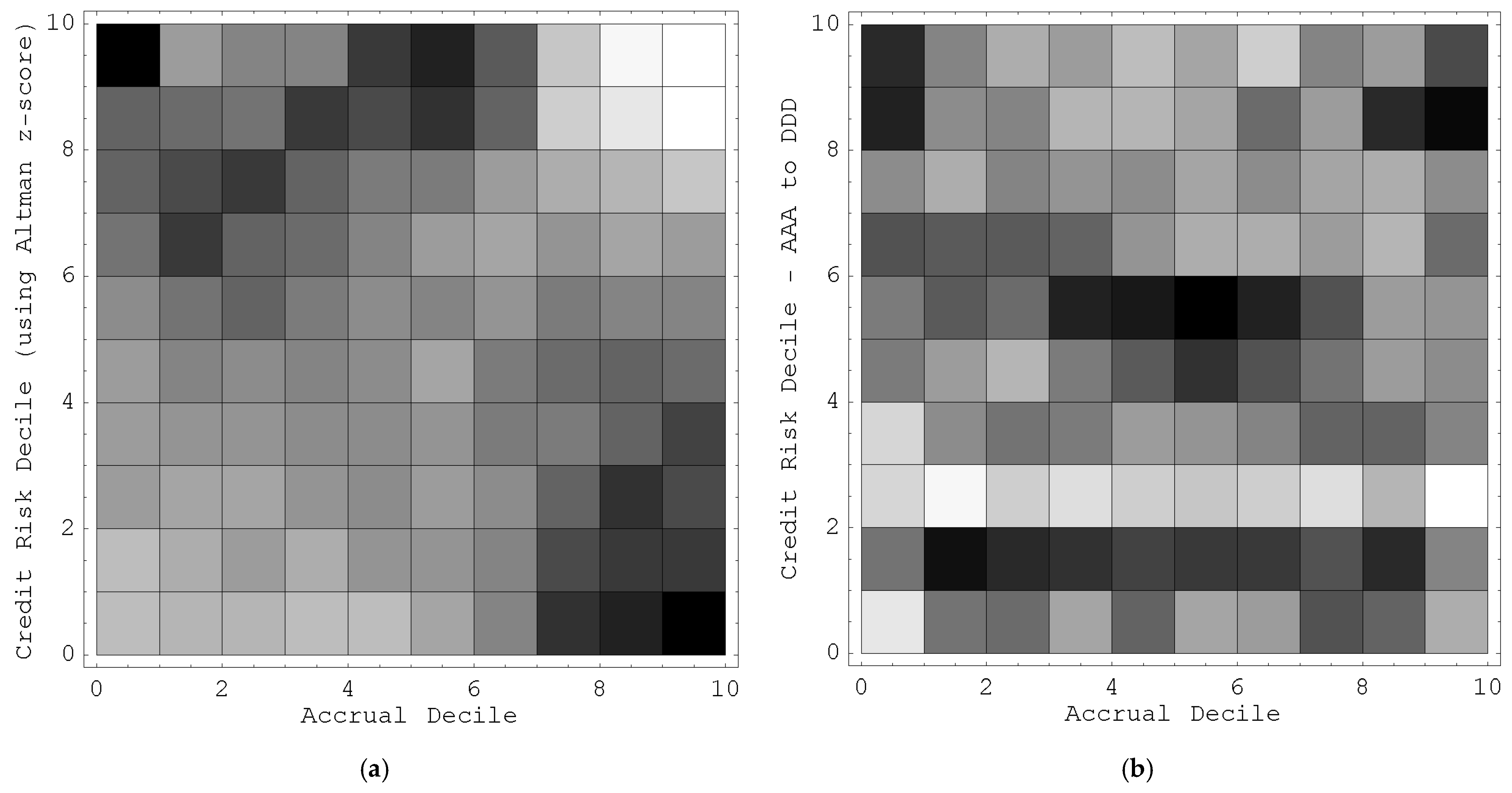
I also provide an intuitive explanation for the results of Hypothesis H1 and H2. First, I partition the firm-year samples into a two-dimensional grid, based on its accrual decile and credit risk decile. Using a two-dimensional density plot, I present the percentage of samples in each of these cells, as well as their mean return. If the first hypothesis is true, I should observe that most of the heavily populated cells lie on the principal diagonal of the grid. If the second hypothesis is true, the mean return from Sloan’s accrual trading strategy should be a decreasing function of its accrual level.

Figure 1a presents the density plot of the percentage of samples, where credit risk is measured using Altman z-score. It is clear from the plot that there is a strong negative correlation between the level of accrual and credit risk.

This density plot is constructed as follows. For each fiscal year, I first rank all the observations into ten deciles by their level of accrual. I also independently rank all the observations into ten deciles of credit risk based on their Altman z-score. I then compute the percentage of firms in each (accrual, credit risk) decile. The intensity of shading for each decile cell varies positively with the time-series mean percentage of firms in that cell. The raw numerical data is available below.

The Spearman rank correlation test reports a statistically significant and negative correlation of −0.19 (p-value is less than 0.01%).

The Altman z-score is computed using Compustat data items: Z = 1.2 (data179/data6) + 1.4 (data36/data6) + 3.3 (data18 + data16 + data15)/data6 + 0.6 (data25 × data199/data181) + (data12/data6).

Figure 1. (a) Density plot of the percentage of firms in each accrual decile and credit risk decile, using Altman z-score, averaged over all years. (b) Density plot of the percentage of firms in each accrual decile and credit risk decile, using Standard & Poor’s credit ratings, averaged over all years. The raw data for this Figure are in Table 5 and Table 6.

Figure 1. (a) Density plot of the percentage of firms in each accrual decile and credit risk decile, using Altman z-score, averaged over all years. (b) Density plot of the percentage of firms in each accrual decile and credit risk decile, using Standard & Poor’s credit ratings, averaged over all years. The raw data for this Figure are in Table 5 and Table 6.

Table 5. Raw data for the density plot in Figure 1a.

	Accrual Decile
Credit Risk Decile	1	2	3	4	5	6	7	8	9	10	Sum
10	1.6%	0.9%	1.0%	1.0%	1.3%	1.5%	1.2%	0.7%	0.4%	0.4%	10.0%
9	1.2%	1.1%	1.1%	1.3%	1.3%	1.4%	1.1%	0.7%	0.5%	0.4%	10.0%
8	1.1%	1.3%	1.3%	1.1%	1.0%	1.0%	0.9%	0.8%	0.7%	0.7%	10.0%
7	1.1%	1.4%	1.2%	1.1%	1.0%	0.9%	0.8%	0.9%	0.8%	0.9%	10.0%
6	0.9%	1.1%	1.1%	1.0%	1.0%	1.0%	0.9%	1.0%	1.0%	1.0%	10.0%
5	0.9%	1.0%	1.0%	1.0%	0.9%	0.8%	1.0%	1.1%	1.1%	1.1%	10.0%
4	0.9%	0.9%	0.9%	1.0%	0.9%	0.9%	1.0%	1.0%	1.1%	1.3%	10.0%
3	0.9%	0.8%	0.8%	0.9%	0.9%	0.9%	1.0%	1.1%	1.4%	1.3%	10.0%
2	0.7%	0.8%	0.9%	0.8%	0.9%	0.9%	1.0%	1.3%	1.4%	1.3%	10.0%
1	0.7%	0.7%	0.8%	0.7%	0.7%	0.8%	1.0%	1.4%	1.5%	1.6%	10.0%
Sum	10.0%	10.0%	10.0%	10.0%	10.0%	10.0%	10.0%	10.0%	10.0%	10.0%	100.0%

Table 5. Raw data for the density plot in Figure 1a.

	Accrual Decile
Credit Risk Decile	1	2	3	4	5	6	7	8	9	10	Sum
10	1.6%	0.9%	1.0%	1.0%	1.3%	1.5%	1.2%	0.7%	0.4%	0.4%	10.0%
9	1.2%	1.1%	1.1%	1.3%	1.3%	1.4%	1.1%	0.7%	0.5%	0.4%	10.0%
8	1.1%	1.3%	1.3%	1.1%	1.0%	1.0%	0.9%	0.8%	0.7%	0.7%	10.0%
7	1.1%	1.4%	1.2%	1.1%	1.0%	0.9%	0.8%	0.9%	0.8%	0.9%	10.0%
6	0.9%	1.1%	1.1%	1.0%	1.0%	1.0%	0.9%	1.0%	1.0%	1.0%	10.0%
5	0.9%	1.0%	1.0%	1.0%	0.9%	0.8%	1.0%	1.1%	1.1%	1.1%	10.0%
4	0.9%	0.9%	0.9%	1.0%	0.9%	0.9%	1.0%	1.0%	1.1%	1.3%	10.0%
3	0.9%	0.8%	0.8%	0.9%	0.9%	0.9%	1.0%	1.1%	1.4%	1.3%	10.0%
2	0.7%	0.8%	0.9%	0.8%	0.9%	0.9%	1.0%	1.3%	1.4%	1.3%	10.0%
1	0.7%	0.7%	0.8%	0.7%	0.7%	0.8%	1.0%	1.4%	1.5%	1.6%	10.0%
Sum	10.0%	10.0%	10.0%	10.0%	10.0%	10.0%	10.0%	10.0%	10.0%	10.0%	100.0%

Figure 1b presents the density plot of the percentage of samples, where credit risk is measured using S&P credit ratings. From the plot, I am unable to infer whether there is a relation between the level of accrual and credit risk. The Spearman rank correlation test reports a statistically insignificant correlation of −0.0051 (p-value equals 0.5883).

Table 6. Raw data for the density plot in Figure 1b.

	Accrual Decile
Credit Risk Decile	1	2	3	4	5	6	7	8	9	10	Sum
10	1.4%	1.0%	0.8%	0.9%	0.7%	0.8%	0.7%	1.0%	0.9%	1.3%	9.4%
9	1.4%	1.0%	1.0%	0.8%	0.8%	0.8%	1.1%	0.9%	1.4%	1.6%	10.7%
8	0.9%	0.8%	1.0%	0.9%	0.9%	0.8%	1.0%	0.8%	0.8%	0.9%	9.0%
7	1.2%	1.2%	1.2%	1.1%	0.9%	0.8%	0.8%	0.9%	0.8%	1.1%	10.0%
6	1.0%	1.2%	1.1%	1.5%	1.5%	1.6%	1.4%	1.2%	0.9%	0.9%	12.3%
5	1.0%	0.9%	0.8%	1.0%	1.2%	1.4%	1.2%	1.1%	0.9%	1.0%	10.4%
4	0.6%	1.0%	1.1%	1.0%	0.9%	0.9%	1.0%	1.2%	1.1%	1.0%	9.7%
3	0.6%	0.5%	0.6%	0.6%	0.6%	0.7%	0.7%	0.6%	0.7%	0.4%	6.0%
2	1.1%	1.5%	1.4%	1.4%	1.3%	1.3%	1.3%	1.2%	1.4%	1.0%	13.0%
1	0.5%	1.1%	1.1%	0.8%	1.1%	0.8%	0.9%	1.2%	1.1%	0.8%	9.5%
Sum	9.9%	10.0%	10.1%	10.0%	10.0%	10.1%	10.0%	10.0%	10.0%	9.9%	100.0%

Table 6. Raw data for the density plot in Figure 1b.

	Accrual Decile
Credit Risk Decile	1	2	3	4	5	6	7	8	9	10	Sum
10	1.4%	1.0%	0.8%	0.9%	0.7%	0.8%	0.7%	1.0%	0.9%	1.3%	9.4%
9	1.4%	1.0%	1.0%	0.8%	0.8%	0.8%	1.1%	0.9%	1.4%	1.6%	10.7%
8	0.9%	0.8%	1.0%	0.9%	0.9%	0.8%	1.0%	0.8%	0.8%	0.9%	9.0%
7	1.2%	1.2%	1.2%	1.1%	0.9%	0.8%	0.8%	0.9%	0.8%	1.1%	10.0%
6	1.0%	1.2%	1.1%	1.5%	1.5%	1.6%	1.4%	1.2%	0.9%	0.9%	12.3%
5	1.0%	0.9%	0.8%	1.0%	1.2%	1.4%	1.2%	1.1%	0.9%	1.0%	10.4%
4	0.6%	1.0%	1.1%	1.0%	0.9%	0.9%	1.0%	1.2%	1.1%	1.0%	9.7%
3	0.6%	0.5%	0.6%	0.6%	0.6%	0.7%	0.7%	0.6%	0.7%	0.4%	6.0%
2	1.1%	1.5%	1.4%	1.4%	1.3%	1.3%	1.3%	1.2%	1.4%	1.0%	13.0%
1	0.5%	1.1%	1.1%	0.8%	1.1%	0.8%	0.9%	1.2%	1.1%	0.8%	9.5%
Sum	9.9%	10.0%	10.1%	10.0%	10.0%	10.1%	10.0%	10.0%	10.0%	9.9%	100.0%

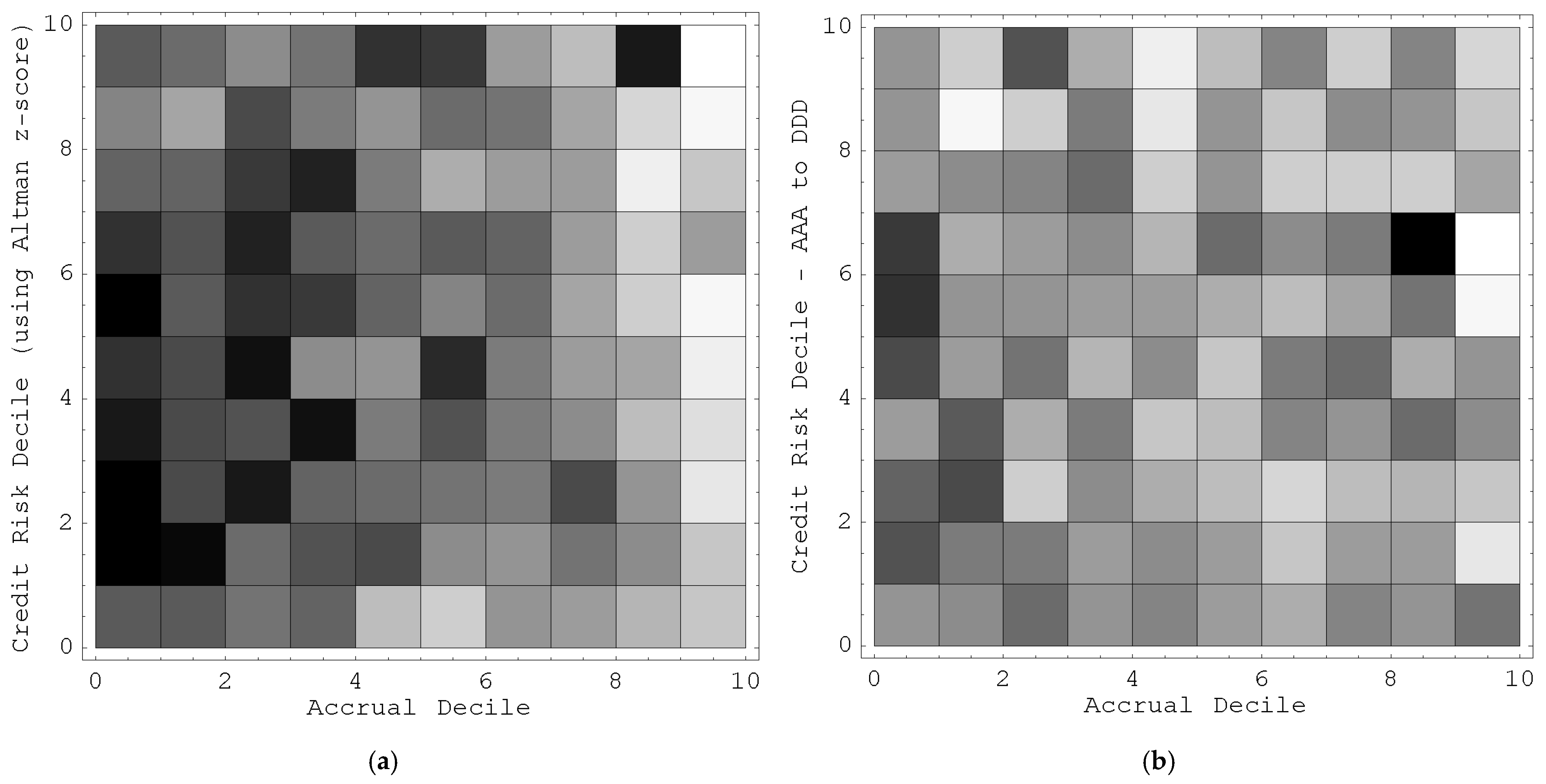
Figure 2a presents the density plot of the mean returns of the samples, where credit risk is measured using Altman z-score. The mean return from the lowest and highest accrual decile is 3.9% and −5.7% respectively. I see a general pattern of decreasing mean return as the level of accrual increases. It is also clear that the leftmost cells in the density plot are generally of higher intensity than the rightmost cells.

This density plot is constructed as follows. For each fiscal year, I first rank all the observations into ten deciles by their level of accrual. I also independently rank all the observations into ten deciles of credit risk based on their Altman z-score. I then compute the cross-sectional mean Size-Adjusted Return (SAR) for the firms in each (accrual, credit risk) cell. The intensity of shading for each cell varies positively with the time-series mean of the cross-sectional mean of SAR. The SAR of a firm is measured as the one-year buy-and-hold return in excess of the buy-and-hold return of the value-weighted portfolio of firms having similar market values (based on the CRSP size deciles for NYSE/AMEX firms). The raw numerical data is available below.

Table 7. Raw data for the density plot in Figure 2a.

	Accrual Decile
Credit Risk Decile	1	2	3	4	5	6	7	8	9	10	Mean
10	1.8%	0.8%	−1.0%	0.5%	4.1%	3.5%	−2.1%	−3.8%	5.5%	−8.0%	0.1%
9	−0.6%	−2.7%	2.6%	−0.3%	−1.5%	0.9%	0.3%	−2.7%	−5.4%	−7.1%	−1.6%
8	1.3%	1.4%	3.6%	5.3%	0.0%	−3.1%	−2.1%	−2.1%	−6.7%	−4.4%	−0.7%
7	4.0%	2.2%	5.0%	1.9%	0.8%	1.8%	1.1%	−2.1%	−4.9%	−2.1%	0.8%
6	7.2%	1.8%	4.1%	3.7%	1.1%	−0.7%	0.9%	−2.7%	−4.9%	−7.5%	0.3%
5	3.9%	2.8%	6.0%	−1.1%	−1.4%	4.6%	−0.2%	−2.3%	−2.7%	−6.7%	0.3%
4	5.5%	2.9%	2.3%	6.1%	−0.3%	2.0%	0.1%	−1.0%	−3.9%	−5.8%	0.8%
3	7.2%	2.5%	5.4%	1.4%	0.7%	0.1%	−0.4%	2.7%	−1.8%	−6.2%	1.2%
2	7.2%	6.3%	0.9%	2.3%	2.6%	−1.1%	−1.4%	0.3%	−0.9%	−4.3%	1.2%
1	1.8%	1.6%	0.4%	1.5%	−4.1%	−5.0%	−1.5%	−2.2%	−3.5%	−4.6%	−1.6%
Mean	3.9%	2.0%	2.9%	2.1%	0.2%	0.3%	−0.5%	−1.6%	−2.9%	−5.7%	0.1%

Table 7. Raw data for the density plot in Figure 2a.

	Accrual Decile
Credit Risk Decile	1	2	3	4	5	6	7	8	9	10	Mean
10	1.8%	0.8%	−1.0%	0.5%	4.1%	3.5%	−2.1%	−3.8%	5.5%	−8.0%	0.1%
9	−0.6%	−2.7%	2.6%	−0.3%	−1.5%	0.9%	0.3%	−2.7%	−5.4%	−7.1%	−1.6%
8	1.3%	1.4%	3.6%	5.3%	0.0%	−3.1%	−2.1%	−2.1%	−6.7%	−4.4%	−0.7%
7	4.0%	2.2%	5.0%	1.9%	0.8%	1.8%	1.1%	−2.1%	−4.9%	−2.1%	0.8%
6	7.2%	1.8%	4.1%	3.7%	1.1%	−0.7%	0.9%	−2.7%	−4.9%	−7.5%	0.3%
5	3.9%	2.8%	6.0%	−1.1%	−1.4%	4.6%	−0.2%	−2.3%	−2.7%	−6.7%	0.3%
4	5.5%	2.9%	2.3%	6.1%	−0.3%	2.0%	0.1%	−1.0%	−3.9%	−5.8%	0.8%
3	7.2%	2.5%	5.4%	1.4%	0.7%	0.1%	−0.4%	2.7%	−1.8%	−6.2%	1.2%
2	7.2%	6.3%	0.9%	2.3%	2.6%	−1.1%	−1.4%	0.3%	−0.9%	−4.3%	1.2%
1	1.8%	1.6%	0.4%	1.5%	−4.1%	−5.0%	−1.5%	−2.2%	−3.5%	−4.6%	−1.6%
Mean	3.9%	2.0%	2.9%	2.1%	0.2%	0.3%	−0.5%	−1.6%	−2.9%	−5.7%	0.1%

Figure 2b presents the density plot of the mean returns of the samples, where credit risk is measured using S&P credit ratings. This density plot is constructed similarly as Figure 2a, using credit rating by Standard & Poor’s. The mean return from the lowest and highest accrual decile is 7.0% and −0.6% respectively. I see a general pattern of decreasing mean return as the level of accrual increases. It is also clear that the leftmost cells in the density plot are generally of higher intensity than the rightmost cells. The raw numerical data is available below in Table 8.

Table 8. Raw data for the density plot in Figure 2b.

	Accrual Decile
Credit Risk Decile	1	2	3	4	5	6	7	8	9	10	Mean
10	3.2%	−1.7%	9.5%	1.4%	−5.2%	−0.7%	5.5%	−1.9%	5.4%	−2.7%	1.3%
9	3.2%	−6.5%	−2.0%	5.9%	−4.1%	3.1%	−1.5%	4.0%	3.2%	−1.2%	0.4%
8	2.8%	4.7%	4.8%	7.8%	−2.3%	3.5%	−2.3%	−2.1%	−1.7%	1.8%	1.7%
7	12.5%	1.3%	3.0%	4.1%	0.7%	7.7%	4.1%	6.0%	18.4%	−7.3%	5.0%
6	13.1%	3.3%	3.1%	2.7%	2.4%	1.3%	−0.2%	1.9%	6.7%	−5.9%	2.8%
5	10.7%	3.0%	6.6%	0.6%	4.3%	−1.5%	6.1%	7.4%	0.7%	3.4%	4.1%
4	2.4%	9.3%	0.9%	5.6%	−1.6%	−0.7%	5.4%	3.8%	7.3%	4.6%	3.7%
3	8.3%	10.9%	−2.3%	4.4%	0.8%	−0.1%	−2.8%	−0.4%	0.5%	−1.6%	1.7%
2	10.3%	5.9%	5.6%	2.7%	4.3%	2.5%	−1.7%	2.8%	3.0%	−4.2%	3.1%
1	3.7%	4.6%	7.8%	3.4%	5.3%	2.3%	1.2%	4.8%	3.6%	7.1%	4.4%
Mean	7.0%	3.5%	3.7%	3.9%	0.4%	1.7%	1.4%	2.6%	4.7%	−0.6%	2.8%

Table 8. Raw data for the density plot in Figure 2b.

	Accrual Decile
Credit Risk Decile	1	2	3	4	5	6	7	8	9	10	Mean
10	3.2%	−1.7%	9.5%	1.4%	−5.2%	−0.7%	5.5%	−1.9%	5.4%	−2.7%	1.3%
9	3.2%	−6.5%	−2.0%	5.9%	−4.1%	3.1%	−1.5%	4.0%	3.2%	−1.2%	0.4%
8	2.8%	4.7%	4.8%	7.8%	−2.3%	3.5%	−2.3%	−2.1%	−1.7%	1.8%	1.7%
7	12.5%	1.3%	3.0%	4.1%	0.7%	7.7%	4.1%	6.0%	18.4%	−7.3%	5.0%
6	13.1%	3.3%	3.1%	2.7%	2.4%	1.3%	−0.2%	1.9%	6.7%	−5.9%	2.8%
5	10.7%	3.0%	6.6%	0.6%	4.3%	−1.5%	6.1%	7.4%	0.7%	3.4%	4.1%
4	2.4%	9.3%	0.9%	5.6%	−1.6%	−0.7%	5.4%	3.8%	7.3%	4.6%	3.7%
3	8.3%	10.9%	−2.3%	4.4%	0.8%	−0.1%	−2.8%	−0.4%	0.5%	−1.6%	1.7%
2	10.3%	5.9%	5.6%	2.7%	4.3%	2.5%	−1.7%	2.8%	3.0%	−4.2%	3.1%
1	3.7%	4.6%	7.8%	3.4%	5.3%	2.3%	1.2%	4.8%	3.6%	7.1%	4.4%
Mean	7.0%	3.5%	3.7%	3.9%	0.4%	1.7%	1.4%	2.6%	4.7%	−0.6%	2.8%

4.4. Test of Hypothesis H3

The final hypothesis tests whether the Size-Adjusted Return is still significant after controlling for credit risk.

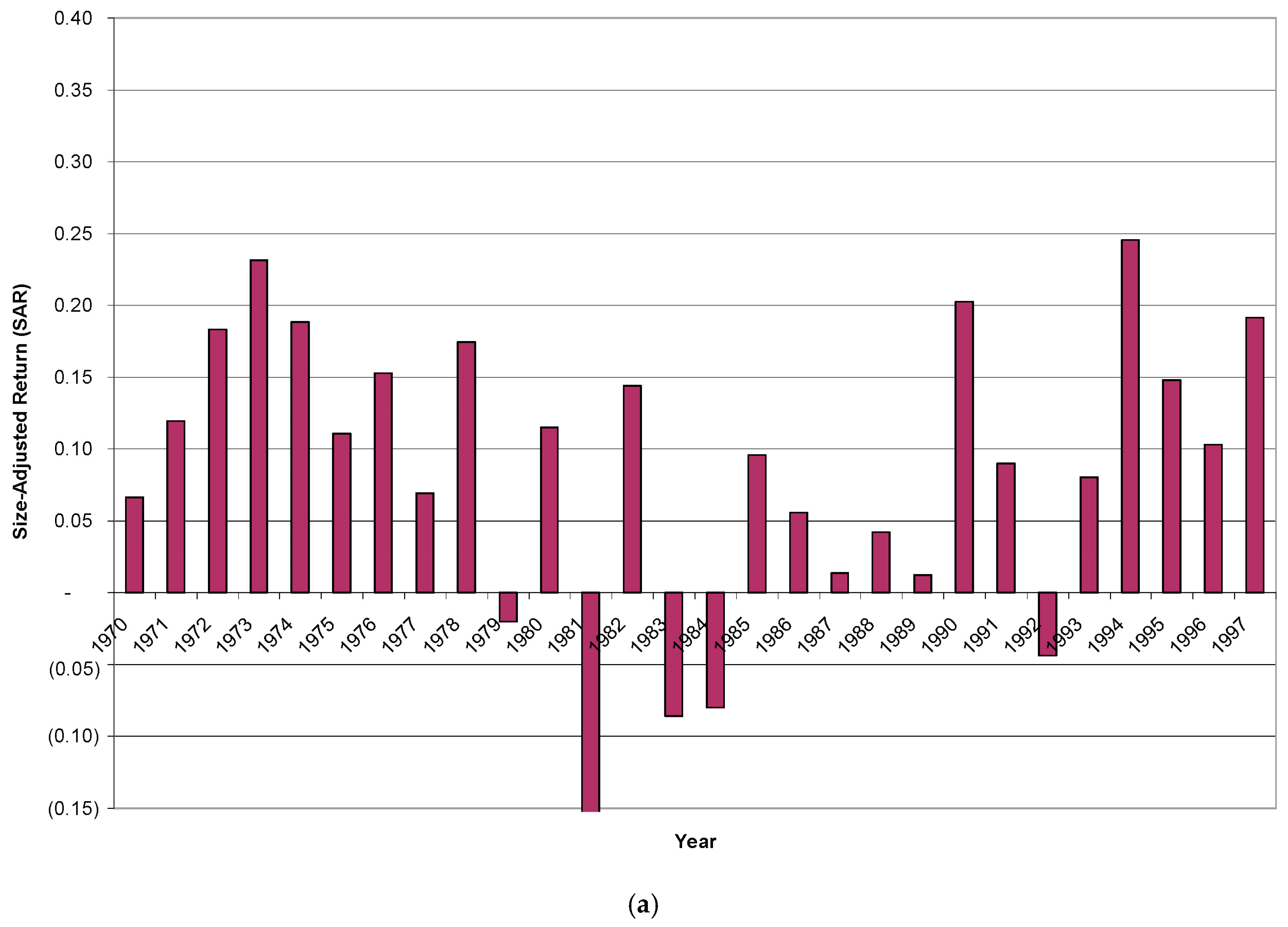
I control for credit risk by requiring that every long position (in the lowest accrual decile) is hedged by a short position (in the highest accrual decile) of the same value in the same credit risk decile. My portfolio is equally weighted across all the credit risk deciles. Figure 3a presents the size-adjusted return (SAR) for this hedge portfolio in each of the 28 years, before controlling for credit risk. The returns are negative only in five out of the twenty-eight fiscal years. 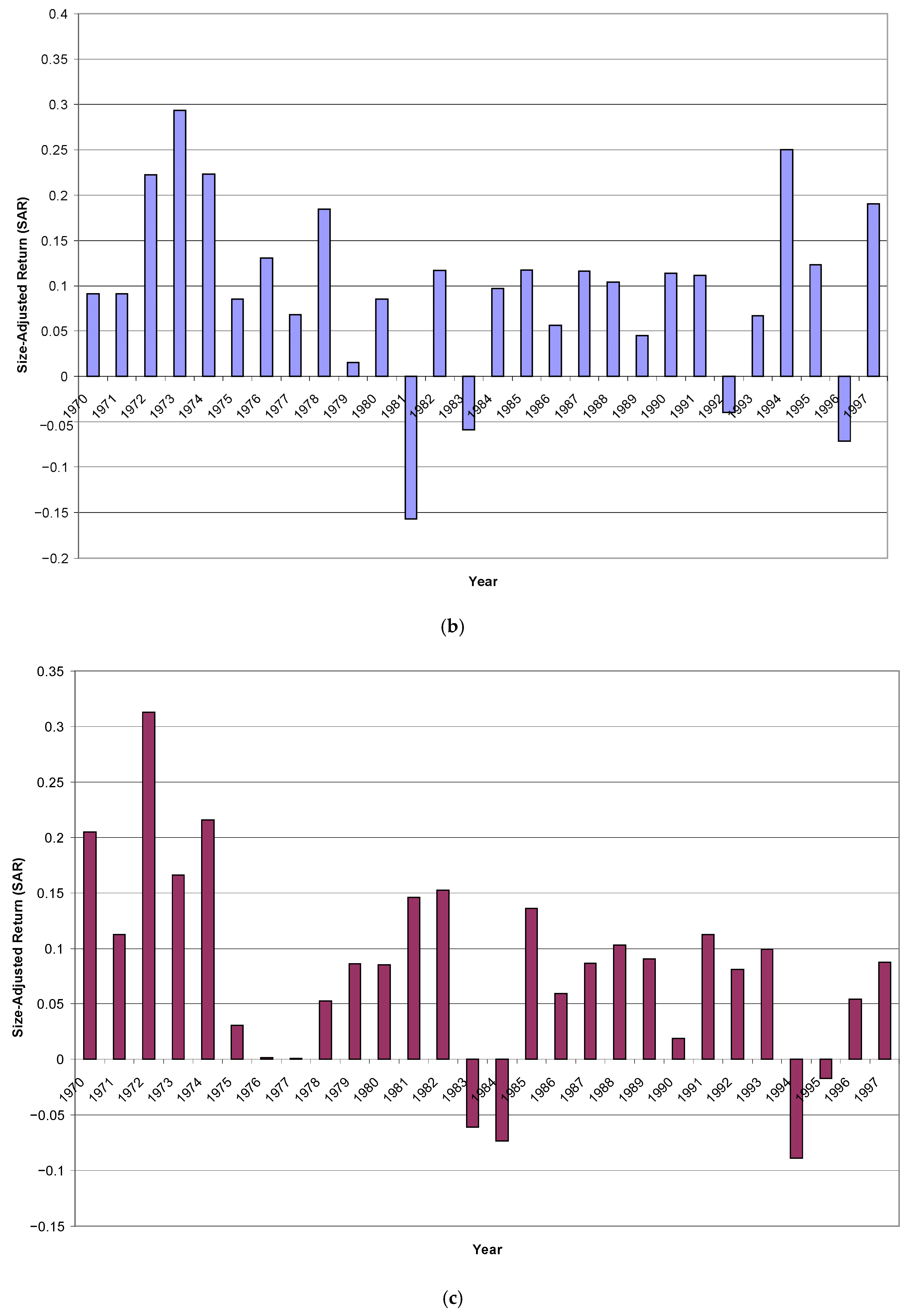Figure 3b presents the SAR for this hedge portfolio in each of the 28 years, where credit risk is measured using Altman z-score. Figure 3c presents the SAR for the hedge portfolio, for the case where credit risk is measured using S&P credit ratings.

In both Figure 3b,c, after controlling for credit risk, I observe that the SAR is positive and statistically significant. The mean SAR is 9.5% and 8.0% respectively. This magnitude is economically large, and is very close to the original mean SAR obtained before controlling for credit risk.

The time-series plot for Figure 3a is constructed as follows. For each fiscal year, I first rank all the observations into ten deciles by their level of accrual. I then compute the cross-sectional mean Size-Adjusted Return (SAR) for the firms in each accrual decile. The SAR of a firm is measured as the one-year buy-and-hold return in excess of the buy-and-hold return of the value-weighted portfolio of firms having similar market values (based on the CRSP size deciles for NYSE/AMEX firms). I require that my portfolio takes a long position in the lowest accrual decile, and a short position of the same value in the highest accrual decile. The SAR reported in the above graph is this hedged return. The time-series mean SAR is 8.8% (significantly positive at 1% level).

This time-series plot for Figure 3b is constructed as follows. For each fiscal year, I first rank all the observations into ten deciles by their level of accrual. I also independently rank all the observations into ten deciles of credit risk based on their Altman z-score. I then compute the cross-sectional mean Size-Adjusted Return (SAR) for the firms in each (accrual, credit risk) decile. The SAR of a firm is measured as the one-year buy-and-hold return in excess of the buy-and-hold return of the value-weighted portfolio of firms having similar market values (based on the CRSP size deciles for NYSE/AMEX firms).

I require that my portfolio takes a long position in the lowest accrual decile, and a short position of the same value in the highest accrual decile. To control for credit risk, I also require that my portfolio to be equally weighted within each credit risk decile. Hence, a long position in the low accrual decile must be offset by a short position of the same value in the high accrual decile in the same credit risk decile. The SAR reported for each year is the equal weighted average of this hedged return obtained for all the ten credit risk deciles. The time-series mean SAR is 9.5% (significantly positive at 1% level).

This time-series plot for Figure 3c is constructed similarly as Figure 3b, using credit rating by Standard & Poor’s. The time-series mean SAR is 8.0% (significantly positive at 1% level).

4.5. Discussion

The empirical analysis demonstrates that the accrual anomaly [1] persists after controlling for credit risk, challenging claims that its abnormal returns reflect a distress risk premium [5,8]. The results support mispricing-based explanations [13,14].

Hypothesis H1 shows that low-accrual firms are not consistently riskier. Altman’s Z-score yields a negative significant correlation with accruals, but S&P credit ratings show no significant link, suggesting Z-score’s overlap with accrual data inflates risk perceptions. Hypothesis H2 confirms accrual drive returns, with significant negative coefficients even after controlling for credit risk. The smaller S&P sample indicates potential selection bias but does not negate the accrual effect.

Graphical analysis (Figure 1) illustrates that Z-score-based plots show a negative accrual–risk link, while S&P plots do not, even though returns consistently decrease with higher accruals. Hypothesis H3’s hedged portfolio, balanced across credit risk deciles, yields significant returns (9.5% for Z-score, 8.0% for S&P, p < 0.01), close to the uncontrolled 8.8%, confirming credit risk’s limited role.

These findings suggest the anomaly stems from investor mispricing, possibly due to accrual distortions [6,14]. Future research could explore behavioral factors or new risk measures using credit default swaps.

5. Conclusions

This study tests whether the abnormal returns of the accrual anomaly, as documented by Sloan [1], reflect a credit risk premium or persist due to other factors, such as mispricing. Using Altman’s Z-score [2] and Standard & Poor’s (S&P) credit ratings [3], I found that the anomaly’s hedge portfolio returns remain positive and statistically significant after controlling for credit risk. These findings are robust across both measures, suggesting that credit risk does not fully explain the accrual anomaly. My results align with mispricing interpretations, as shown, e.g., in [13,14], but do not preclude other risk factors. For instance, Campbell et al. [15] found that distressed stocks underperform, challenging the theory of a simple distress risk premium. My contribution lies in directly testing and rejecting the credit risk hypothesis, providing evidence that the accrual anomaly is more likely driven by investor mispricing or unmodeled factors than by credit-related risk. This aligns with studies suggesting that accrual distortions may lead to market mispricing, reinforcing the notion that unreliable financial reporting contributes to the anomaly’s persistence.

Future research could explore additional risk factors (e.g., credit default swap) or behavioral explanations, such as investor inattention to accrual reliability, to further explain the anomaly’s persistence. My study contributes to the ongoing debate between risk- and mispricing-based explanations [16,17,18,19,20,21,22,23,24,25,26], with implications for investors and regulators seeking to understand accounting-based anomalies.