Numerical Simulation Research on Thermoacoustic Instability of Cryogenic Hydrogen Filling Pipeline

Abstract

This article uses FLUENT to construct a two-dimensional axisymmetric numerical model of a cryogenic hydrogen charging pipeline. By loading with initial temperature gradient and transient initial pressure disturbance, the basic characteristics of low-temperature hydrogen Taconis thermoacoustic oscillation are calculated, including temperature, heat flux density distribution, pressure amplitude, and frequency. The instability boundary of hydrogen TAO is also obtained. The results show that (1) the temperature distribution and flow characteristics of the gas inside the pipeline exhibit significant periodic changes. In the first half of the oscillation period, the cold-end gas moves towards the end of the pipeline. Low-viscosity cold hydrogen is easily heated and rapidly expands. In the second half of the cycle, the expanding cold gas pushes the hot-end gas to move towards the cold end, forming a low-pressure zone and causing gas backflow. (2) Thermoacoustic oscillation can also cause additional thermal leakage on the pipeline wall. The average heat flux during one cycle is 1150.1 W/m² for inflow and 1087.7 W/m² for outflow, with a net inflow heat flux of 62.4 W/m². (3) The instability boundary of the system is mainly determined by the temperature ratio of the cold and hot ends α, temperature gradient β, and length ratio of the cold and hot ends ξ. Increasing the pipe diameter and minimizing the pipe length can effectively weaken the amplitude of thermoacoustic oscillations. This study provides theoretical support for predicting thermoacoustic oscillations in low-temperature hydrogen transport pipeline systems and offers insights for system stability control and design verification.

1. Introduction

Taconis thermoacoustic oscillation (TAO) refers to the oscillation phenomenon of mutual conversion between thermal energy and acoustic energy caused by temperature changes in low-temperature environments. Taconis first discovered this phenomenon and pointed out that this oscillation would significantly affect the heat leakage in the cryogenic system and the stability of thermodynamic parameters such as temperature and pressure; subsequently, the linear thermoacoustic theory proposed by Rott deepened the understanding of the essence of thermoacoustics and laid the foundation for the quantitative description of TAO [1]. Sugimoto et al. [2,3] proposed a boundary layer theoretical framework for simulating thermoacoustic oscillations; they divided the Taconis tube into the mainstream region and the boundary layer region and successfully simulated the oscillation of the fixed physical properties of helium in a quarter-wavelength tube with a one-dimensional thermoacoustic equation. Ishigaki et al. [4,5] studied the temperature ratio parameters of vibration initiation and vibration elimination under different initial pressures by using a higher precision discrete format based on linear theory and the CFD method. In addition, Lobanov [6] studied a superconducting linac in practical engineering and found that TAO would be generated in three places, namely a cryogenic liquid helium level sensor, a helium-filled precooling pipeline, and a cryogenic distribution valve box with a transmission pipe. Guo et al. [7] used a numerical simulation method to reveal the generation mechanism of TAO, using helium as the working fluid. Jiang et al. [8] analyzed the generation conditions of TAO and proposed the idea of using an existing critical oscillation curve to design and check the connecting pipeline of a liquid helium container from an engineering point of view. Wang et al. [9] studied the TAO characteristics of different inner diameter half-open Taconis tubes in superfluid helium through experiments. Hu et al. [10,11] revealed the nonlinear characteristics of TAO in a helium system by using CFD simulation and nonlinear theory research and analyzed the methods of suppressing thermoacoustic oscillation from the perspective of nonlinear dynamics.

Hydrogen has the absolute advantage of high specific energy and will play an important role in large-scale hydrogen energy applications in the future [12]. Low-temperature liquid hydrogen involves numerous structural components and complex thermodynamic behaviors in various stages of “production–storage–transportation–use”. Improper pipeline structure design is highly likely to cause TAO. However, the current research on TAO is mainly focused on liquid helium systems, and the research on cryogenic hydrogen systems is still insufficient. Only Gu et al. [13,14] calculated the stability curves of three-phase point hydrogen and standard hydrogen under step temperature distribution. Matveev et al. [15] used Simcenter Star CCM+ software version 2022.1 to conduct thermoacoustic modeling and used a CFD model on low-temperature hydrogen with real fluid characteristics. Shenton et al. [16] studied the thermoacoustic oscillation boundaries of hydrogen and helium in U-shaped tubes through theoretical analysis and experimental research. Sun et al. [17] used a CFD model to comparatively analyze the generation mechanism of thermoacoustic oscillations in helium and hydrogen.

To further understand the characteristics and stability limits of TAO in cryogenic hydrogen pipelines, a half-open and half-closed cryogenic hydrogen pipeline model was constructed using FLUENT21.2. The fundamental oscillation characteristics of hydrogen TAO, including pressure variations and oscillation frequencies, were determined. The impacts of the temperature gradient, temperature ratio between the hot and cold ends, length ratio of the hot and cold sections, pipe diameter, and pipe length on the stability limit of hydrogen TAO were comparatively analyzed. This research can offer theoretical support for predicting thermoacoustic oscillations in cryogenic hydrogen transportation pipeline systems and provide references for system stability control and design verification.

2. Numerical Model

2.1. Model Description and Simplification

The cryogenic liquid hydrogen filling system includes a cryogenic tank, cryogenic pipeline, cryogenic valve, and discharge system. In fact, under different working conditions, such as when the valve is closed, some pipe sections of the cryogenic filling system may become blind pipe sections. If the pipeline lacks an insulation layer and has thin walls, a significant temperature gradient can easily form along the pipe wall in the blind section. When low-temperature hydrogen is filled into the pipeline and is subjected to minor disturbances such as changes in velocity or pressure, high-frequency spontaneous pressure oscillations may occur. This phenomenon is known as low-temperature thermoacoustic oscillation instability. When TAO occurs in low-temperature hydrogen, its oscillation frequency can cause noise and resonance with other structures. This self-excited oscillation may also lead to additional heat leakage and interfere with pressure measurements. If this instability is not fully considered in the design, it may result in structural damage and pose a threat to the safety of liquid hydrogen transportation. Therefore, it is essential to investigate the distribution patterns and influencing factors of TAO pressure and frequency.

After simplifying the physical model, a two-dimensional axisymmetric model was constructed for the cryogenic hydrogen blind tube pipeline shown in Figure 1, with a pipeline length of L = 1 m, an inner diameter of D = 20 mm, and a wall thickness of 1 mm. Assuming that the open end (x = 0) is in a low-temperature environment, it represents a low-temperature state in the liquid hydrogen temperature zone, such as being connected to a liquid hydrogen container and transporting liquid hydrogen in full. The temperature is taken as T_L = 20 K. The closed end (x = L) is in a normal temperature environment, characterized by no pre-cooling, local heat leakage, and temperature rise, with T_H = 300 K. The position of the maximum temperature gradient along the wall of the pipe is x_m.

2.2. Governing Equations

The governing equations of FLUENT used to solve the continuity, momentum, and energy for the working medium in the computational model are as follows:

2.2.1. Continuity Equations

$${\displaystyle \frac{\partial \rho }{\partial t}}+\nabla (\rho \overrightarrow{V})=0$$

(1)

where $\overrightarrow{V}=u\overrightarrow{i}+v\overrightarrow{j}$ represents velocity vector, $\overrightarrow{i}$ and $\overrightarrow{j}$ comprise the unit coordinate vector, the density ρ is calculated based on the ideal gas state equation $p=\rho R_{g}T$, and R_g is the hydrogen gas constant.

2.2.2. Momentum Equation

$${\displaystyle \frac{\partial (\rho \overrightarrow{V})}{\partial t}}+\nabla (\rho \overrightarrow{V})\overrightarrow{V}=-\nabla p+\nabla \mathrm{\Pi }$$

(2)

where μ is the dynamic viscosity, p is the pressure of gas, and Π is the viscous stress tensor, $\mathrm{\Pi }=[\mu ({\displaystyle \frac{\partial u}{\partial y}}+{\displaystyle \frac{\partial v}{\partial x}})]$.

2.2.3. Energy Balance Equations

$${\displaystyle \frac{\partial (\rho E)}{\partial t}}+\nabla ((\rho E+p)\overrightarrow{V})=k{\nabla }^{2}T+\nabla (\overrightarrow{V}\cdot \mathrm{\Pi })$$

(3)

where E is the internal energy of the gas; the expression is $E=h-{\displaystyle \frac{p}{\rho }}+{\displaystyle \frac{{\left|\overrightarrow{V}\right|}^2}{2}}$.

2.3. Boundary Condition

In order to solve the whole process of thermoacoustic oscillation, it is necessary to set the initial temperature field. Set the initial condition such that the temperature of the whole field along the pipe length is T_x by loading the user-defined function (UDF) [7]:

$$A(x)={\displaystyle \frac{1}{2}}(\tanh (\beta (x-x_{\max })))-{\displaystyle \frac{1}{2}}(\tanh (\beta (x+x_{\max })))+1$$

(4)

$$B(x)={\displaystyle \frac{A(x)+A(2L-x)-1}{2A(L)-1}}$$

(5)

$$T_{\mathrm{x}}=T_{\mathrm{H}}({\displaystyle \frac{B(x)-B(0)}{1-B(0)}}+{\displaystyle \frac{1-B(x)}{(1-B(0))\alpha }})$$

(6)

where β is the temperature gradient, x is the distance from the open end of the pipe, α is the temperature ratio of the hot and cold ends, and ξ is the length ratio of the hot and cold ends. The temperature distribution form shown in Figure 2 can be obtained through the above function settings. Different temperature distribution curves can be formed by changing α, β, and x_max.

After setting the initial temperature field conditions, the transient calculation of the disturbance development process is carried out by applying a small pressure disturbance to the whole field. This paper chooses to apply a sinusoidal form of transient initial pressure disturbance [17]:

$$p=150\sin ({\displaystyle \frac{\pi x}{2L}})$$

(7)

The two-dimensional axisymmetric model is structured and meshed by ICEM, and the boundary layer is meshed near the wall using the FLUENT21.2 pressure-based solver. The standard k-ε turbulence model is selected to describe the flow characteristics in the pipe. Considering the compressibility of gas oscillation, the ideal gas model was selected. The thermal conductivity and dynamic viscosity changed with temperature and were fitted based on the NIST database. The initial pressure and operating pressure are set to 101,325 Pa, the wall condition without sliding is selected for the inner wall, and the pressure outlet boundary is selected for the open end (x = 0). The coupled model is used for transient calculations, and the pressure discrete format is PRESTO!. The second-order implicit scheme is used for time discretization, and the second-order upwind scheme is used for other terms. In the process of a transient iterative solution for each time step, the convergence value of the energy residual is 10⁻⁸ and the convergence value of the continuity residual and velocity residual is 10⁻⁵. When the residual is less than the corresponding convergence value, the next time step is entered.

3. Model Validation

3.1. Grid/Time Step Independence Verification

Using the same division method, only changing the grid size, controlling the grid length along the pipe length direction to 1 mm, changing the axial grid size to densify the boundary layer, and establishing four calculation models with different grid numbers (68,204, 78,312, 88,264, and 108,324) can be used to verify the grid independence. Under the same calculation conditions, the variation curves of the pressure and frequency at the pipeline end at different time steps when reaching the stable oscillation state are shown in Figure 3a. From the black circle in the figure, it can be seen that the models using 88,264 grids and 108,324 grids have almost no difference in the development laws and specific values of pressure and frequency. Therefore, it is considered that the current selected grid numbers are sufficient for the numerical simulation of this problem and achieve satisfactory grid density.

Using the 88,264 grid number calculation model, only the time step is changed to verify the independence. Under the same calculation condition, the fluctuation curve of the pressure at the end of the pipeline with time, when it basically reaches the steady state under different time steps, is shown in Figure 3b. It can be seen from the figure that the calculation results of the model using 0.1 ms and 0.05 ms have little difference in the development law of pressure fluctuation and specific values, and it is considered that the numerical simulation of the problem with the time step of 0.1 ms has achieved satisfactory results.

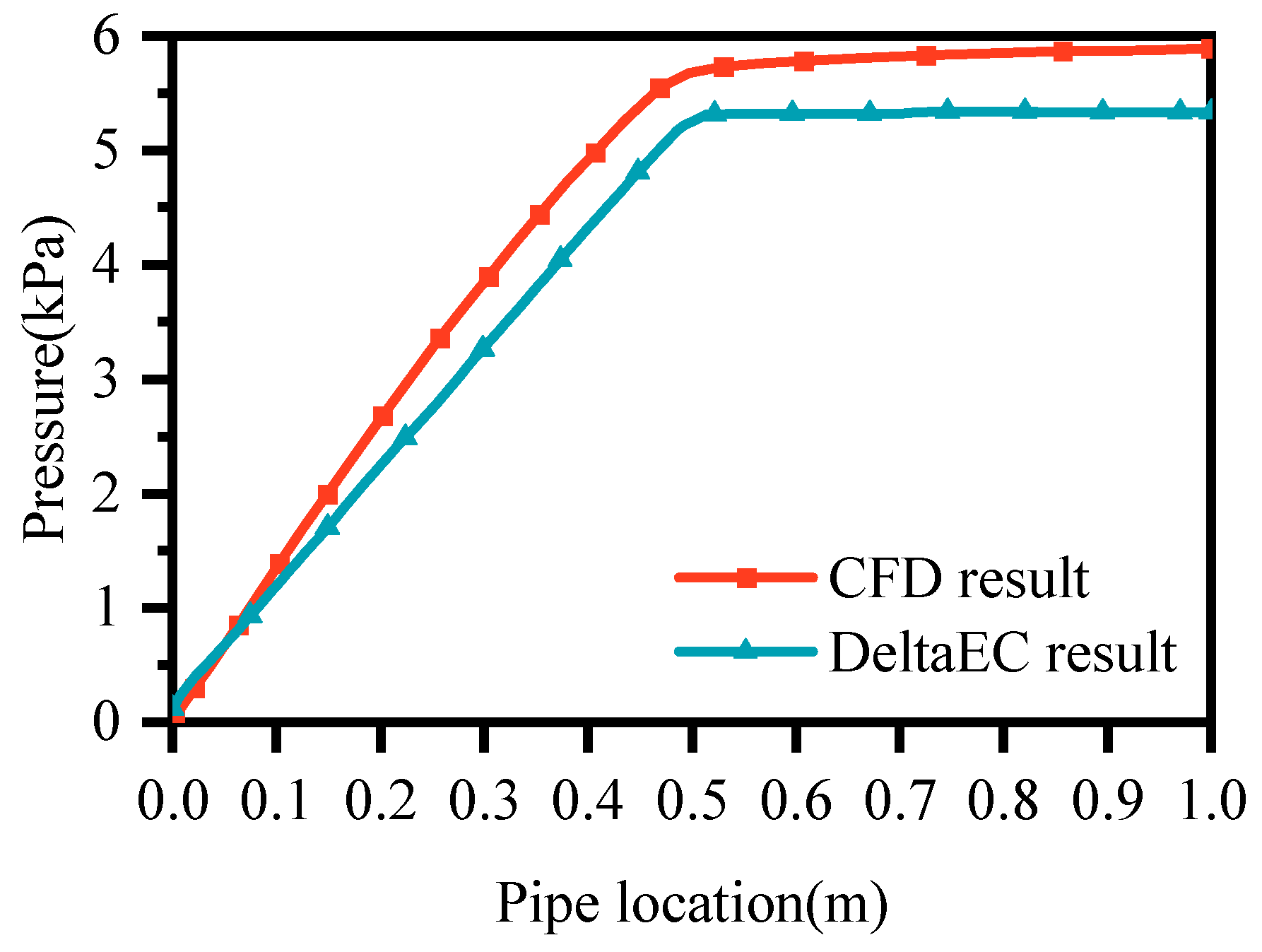
3.2. Qualitative and Quantitative Verification

Since there is no public literature on low-temperature hydrogen TAO experimental data, the existing research only focuses on system stability, and there is limited detailed data such as TAO amplitude and frequency, this paper selects the hydrogen simulation results in [14] and the helium experimental data in [18] as a comparison and uses the (no) oscillation consistency of the corresponding working conditions as the criterion to carry out model verification (both use the same pipe length as the literature).

As depicted in Figure 4a,b, points A, B, C, and D were chosen on both sides of the hydrogen and helium oscillation stability curves for verification and calculation. The results obtained were consistent with the literature, indicating that points A and C did not oscillate while points B and D did. This confirms that the model presented in this paper can effectively calculate TAO characteristics and is applicable to a range of working fluids and conditions.

Point B was selected for quantitative verification. DeltaEC, which is a linear thermoacoustic simulation software program specifically designed for thermoacoustic systems, is widely employed in the field of thermoacoustic simulations. Figure 5 shows the pressure amplitude distribution obtained by CFD and DeltaEC; the difference is basically less than 15%. Therefore, we can consider that the CFD model adopted in this paper is reliable both qualitatively and quantitatively.

4. Results and Discussion

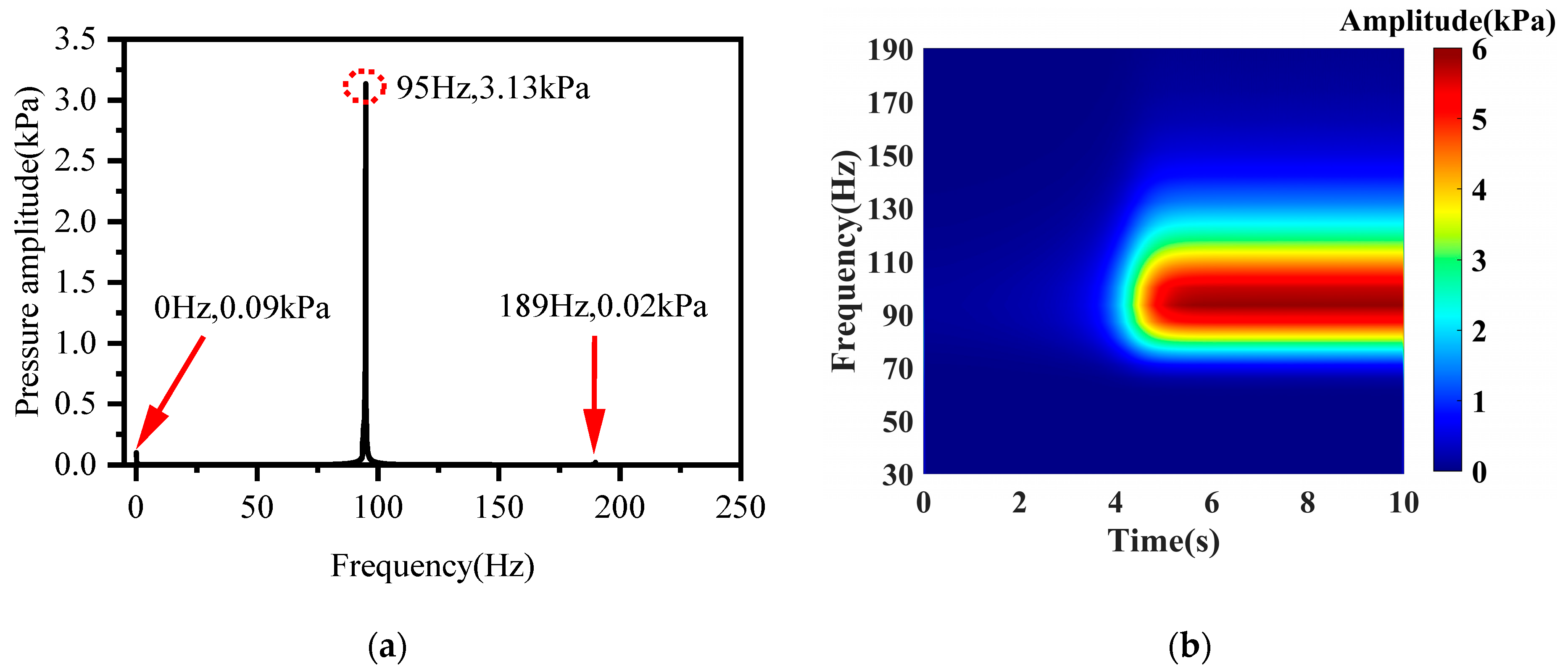
4.1. Basic Characteristic Analysis

The above-mentioned CFD model was used to calculate the starting process of low-temperature hydrogen working fluid under the working conditions of pipe length L = 1 m, pipe diameter D = 20 mm, temperature gradient β = 100 K/m, hot- and cold-end temperature ratio α = 15, and hot- and cold-end length ratio ξ = 1. The complete starting process is shown in Figure 6. It can be seen that there is always oscillation fluctuation in the pressure at the end of the pipeline, and the amplitude increases continuously with time in the initial stage. After about 3 s, the pressure oscillation reaches relative stability. The oscillation development process has a period of approximately 0.0106 s and a frequency of 94.3 Hz.

Figure 7a shows the amplitude–frequency characteristics of the pressure at the end of the pipeline. The result of performing fast Fourier transform (FFT) on the entire pressure oscillation signal shows that the amplitude at frequency 0 is 0.09 kPa, corresponding to the DC component in the oscillation. It also shows that the main frequency of the pressure oscillation is 95 Hz and the amplitude is 3.13 kPa. At the same time, there exists a second frequency with an amplitude of only 0.02 kPa and a frequency of 189 Hz. Figure 7b shows the time–frequency characteristics of the pressure at the end of the pipeline. It is the result obtained by applying MATLAB 2024a’s built-in continuous wavelet transform (CWT) to the pressure oscillation signal. It can be seen that the oscillation signal is a typical non-stationary signal, and the amplitude and frequency of the oscillation continue to increase over time, eventually reaching a stable stage and forming oscillations with different frequencies and amplitudes superimposed.

4.2. Pipe Wall and Fluid Temperature Distribution

After the pressure amplitude stabilizes, the temperature change within one oscillation cycle can be obtained. Figure 8 shows the stage division of periodic pressure oscillation, and the temperature distribution of the pipeline at different times when the oscillation process reaches a stable state is shown in Figure 9.

Within the time range of 0–4.9 ms, which belongs to the first half cycle of oscillation, it can be seen that the cold-end gas in the tube is moving towards the end of the pipeline. Due to the low viscosity of the cold-end gas, it is easy for the cold gas to move, and the significant axial temperature gradient will cause the cold gas to be heated, and it will rapidly expand. During the period from 4.9 ms to 10.5 ms, which corresponds to the latter half of the oscillation cycle, the expanding cold gas pushes the gas from the hot end into the cold end of the tube. If the inertial force is large enough, a low-pressure zone will form in the hot end of the tube. This is due to the inertial motion and the drastic changes in gas density. The low pressure in the hot end causes the dense gas in the cold end to flow back to the hot end in reverse, repeating this cycle. If the driving force exceeds the dissipation effect, it will ultimately lead to TAO. The entry of cold gas increases the radial temperature gradient at the hot end. As the gas moves axially, the heat exchange of the radial significantly increases and becomes dominant.

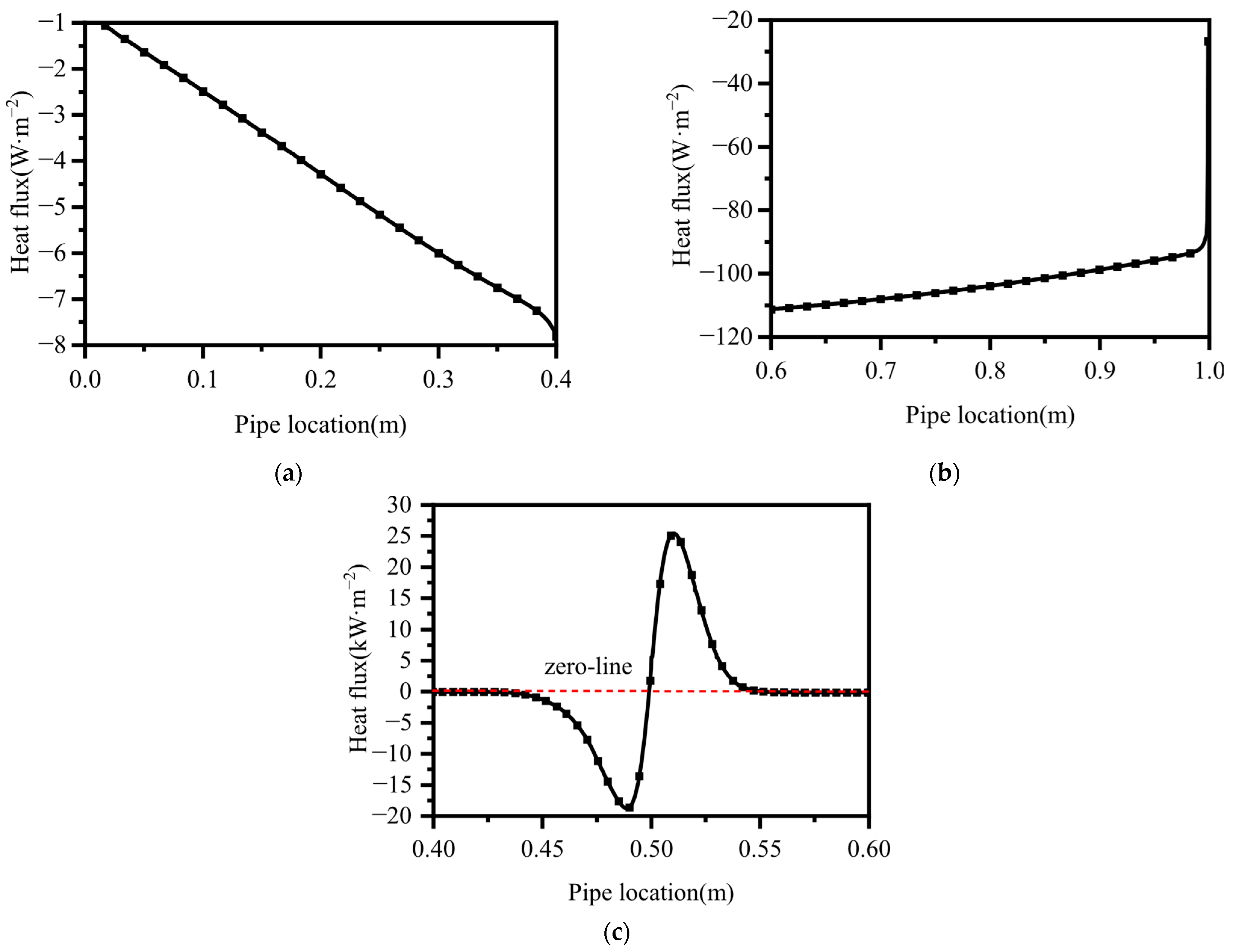
4.3. Analysis of Heat Flux Density of Pipe Wall

In order to analyze the radial heat flux distribution along the wall in the process of thermoacoustic oscillation in detail, the heat flux density along the inner wall of the pipe at each time step can be obtained by post-processing the data derived from FLUENT with MATLAB. The time-averaged heat flux density of different parts of the pipe passing through the inner wall can be obtained by time-average processing the data over a period of time. A positive value indicates that the heat flows into the pipe, and a negative value indicates that the heat flows out. The calculation formula for the hourly average heat flux is as follows:

$$\overline{q}={\displaystyle \frac{1}{T}}{\displaystyle {\int }_0^T{q}_t\mathrm{d}t}$$

(8)

As shown in Figure 10, it can be seen from the figure that the hourly average heat mainly flows in from the middle of the pipe and out from both ends of the pipe.

The heat flux density in the middle of the pipe is much higher than that at both ends, and the negative heat flux density at both ends also shows that the pipe with thermoacoustic oscillation will generate additional heat leakage at the cold end. The time-averaged heat flux is 1150.1 W/m² for the inflow fluid, 1087.7 W/m² for the outflow, and 62.4 W/m² for the net inflow fluid, which is greater than zero. This part of heat means the thermoacoustic oscillation can be maintained.

4.4. Research on Stability Limit

In practical engineering, there is a lot of attention paid to whether the pipeline is in a stable state, and the maximum amplitude and frequency of pressure in the pipeline are usually used to characterize the stability of the system. This paper selects five key influencing factors (see Figure 2), namely the temperature ratio of cold and hot ends α, temperature gradient β, length ratio of cold and hot ends ξ, pipe diameter D, and pipe length L, for variable operating condition calculations.

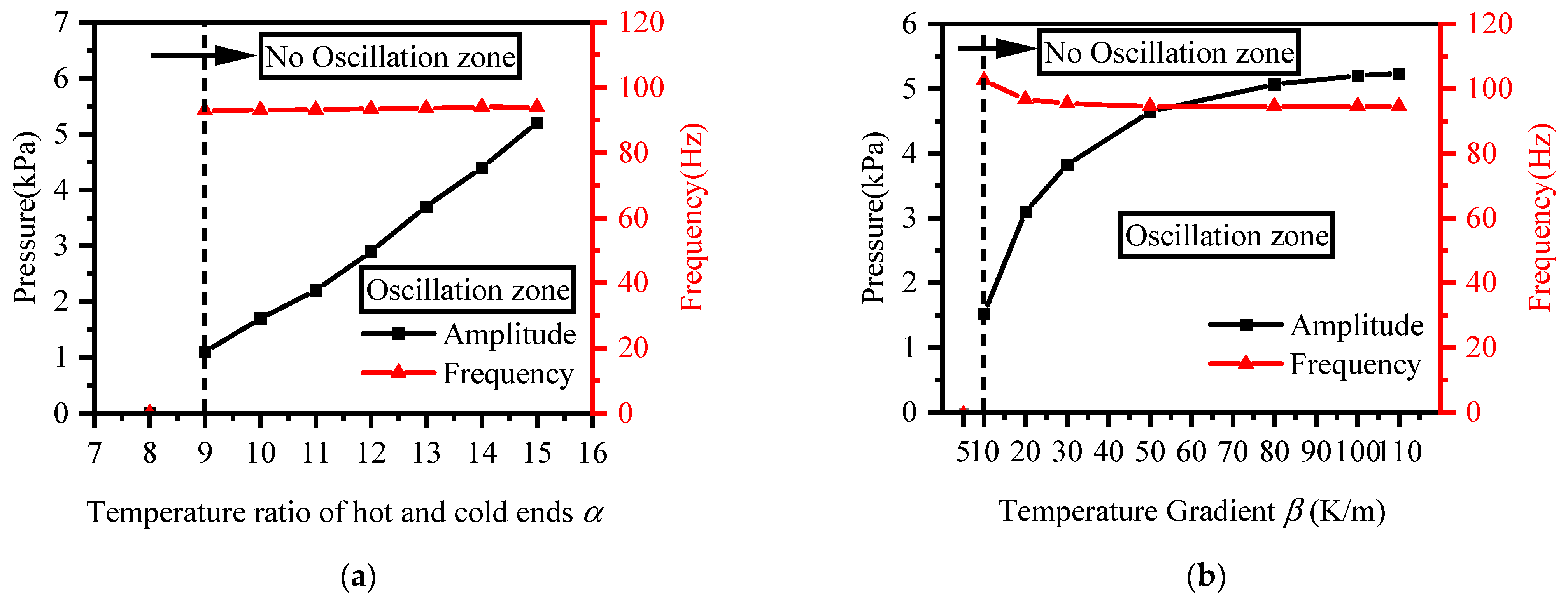
4.4.1. Influence of Temperature

Keeping the temperature gradient β = 100 K/m, the length ratio of the hot and cold ends ξ = 1, and the pipe diameter D = 20 mm unchanged, calculate α = 8 (160 K/20 K) to 15 (300 K/20 K) and obtain the variation characteristics of amplitude and frequency with the temperature ratio of the hot and cold ends, as shown in Figure 11a. Keeping the pipe diameter D = 20 mm, the temperature ratio of the hot and cold ends α = 15 (300 K/20 K) and the length ratio of the hot and cold ends ξ = 1 unchanged, β = 5 to 110 K/m was taken for calculation. The variation characteristics of amplitude and frequency with the temperature gradient are shown in Figure 11b.

The influence of the temperature gradient on thermoacoustic instability is first reflected in whether thermoacoustic oscillations will occur. From Figure 11a, it can be seen that there is a stability boundary for the temperature ratio of the hot and cold ends compared to α. When α < 9 (180 K/20 K), the system will not oscillate. When α ≥ 9, the system will oscillate above the critical temperature ratio; as α increases, the maximum amplitude continues to rise approximately in a linear relationship, while the frequency remains relatively unchanged. From Figure 11b, it can be seen that there is a stability boundary for the temperature gradient β, and the critical value for this operating condition is β = 10 K/m. The reason is that according to thermoacoustic theory, a non-zero temperature gradient will form a controlled source term for the volumetric flow rate. As β further increases, the frequency eventually stabilizes around 95 Hz, indicating that the temperature gradient has little effect on the frequency.

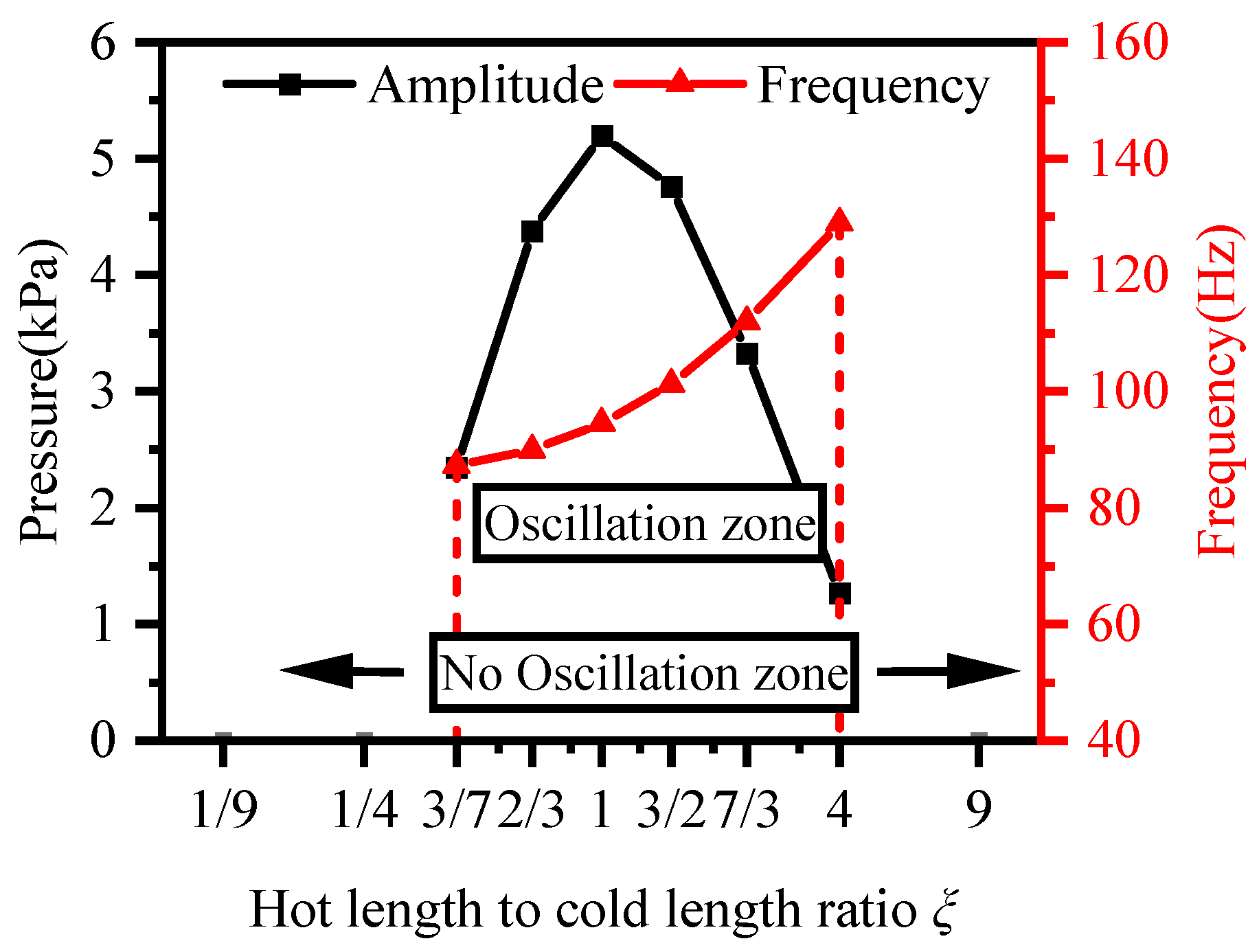
4.4.2. Influence of Ratio of Hot Length to Cold Length

Keeping the pipe diameter D = 20 mm, the temperature ratio between the hot and cold ends α = 15 (300 K/20 K), and the temperature gradient β = 100 K/m constant, calculate using ξ = 1/9~9. The variation characteristics of amplitude and frequency with the length ratio of the hot and cold ends are shown in Figure 12.

From Figure 12, it can be seen that there are two stability limits for the length ratio ξ of the hot and cold ends. The corresponding critical values for this operating condition are ξ = 3/7 and ξ = 4, dividing it into one oscillation zone and two no-oscillation zones. In order to demonstrate the pattern more clearly, logarithmic coordinates are used to describe the horizontal axis. When the hot length is relatively short compared to the cold length (ξ < 3/7), the system is in the no oscillation zone. In this zone, due to the fact that the density of gas inside the tube at low temperatures is much higher than that at room temperature, the system oscillation can be regarded as a mass spring system. The gas in the low-temperature section can be regarded as a mass block, while the gas in the high-temperature section can be regarded as a spring. At this time, the mass of the gas in the cold end is larger, the inertia force is greater, the length of the hot end is shorter, and the driving force is insufficient. Therefore, the system is less likely to oscillate. When the hot length increases to a certain extent (3/7 < ξ < 4), the system enters the oscillation zone. In this zone, the heat transfer process becomes unstable. The heat transfer rate in the hot section increases, leading to higher pressure in that section. The pressure difference between the hot and cold sections creates a pressure wave, causing the pressure amplitude to increase sharply to a peak and then decrease slightly. At the same time, the frequency increases gradually. As the hot length continues to increase beyond a certain point (ξ > 4), the system’s geometry and heat transfer characteristics change again. At this time, the gas length in the high-temperature section is relatively long and the loss caused by viscous force is greater, so the system is less prone to oscillation.

4.4.3. Influence of Geometric Parameters of Pipeline

Keeping the temperature gradient β = 100 K/m, the temperature ratio of the hot and cold ends α = 15 (300 K/20 K), and the length ratio of the hot and cold ends ξ = 1 unchanged, D = 5 mm to 20 mm was taken for calculation. The variation characteristics of amplitude and frequency with pipe diameter are shown in Figure 13a. Keeping the pipe diameter D = 20 mm, the temperature gradient β = 100 K/m, the temperature ratio of the hot and cold ends α = 15 (300 K/20 K), and the length ratio of the hot and cold ends ξ = 1 unchanged, L was taken as 0.5 m, 0.6 m, 0.8 m, and 1 m for calculation. The variation characteristics of amplitude and frequency with pipe length are shown in Figure 13b.

Within the scope of the working conditions studied in this article, changing the pipeline structure will not generate stability boundaries. From Figure 13a, it can be seen that as the diameter of the pipe increases, there is a decreasing trend in both the frequency and amplitude of pressure oscillations, and the attenuation rate is higher in the small diameter region (D < 12 mm) than in the large diameter region (D > 12 mm). According to thermoacoustic theory, oscillations are suppressed when the pipe diameter is large because the boundary layer thickness is relatively thin compared to the pipe diameter and the gas inertia is large, requiring a large driving force to overcome the inertial force. The increase in pipe diameter in engineering is much greater than the thickness of the boundary layer, so when the pipe diameter is small, it is easier to weaken oscillations by increasing the pipe diameter, while when the pipe diameter is large, this weakening effect is no longer significant. From Figure 13b, it can be seen that the length of the pipe has a significant impact on both amplitude and frequency. The length of the pipe is approximately inversely proportional to frequency and approximately proportional to amplitude. Therefore, high-frequency oscillations with lower amplitudes are more likely to occur in shorter pipelines.

5. Conclusions

In order to master the characteristics of TAO in a low-temperature hydrogen transmission pipeline, the authors built a two-dimensional semi-open and semi-closed pipe simulation model to calculate the onset process of the low-temperature hydrogen pipeline, and they analyzed the influence of many factors on the oscillation characteristics. The main conclusions are as follows:

• The FLUENT numerical solver was used to numerically simulate and analyze the TAO of cryogenic hydrogen, and the entire TAO process was successfully achieved. By comparing with other experiments, it is demonstrated that the model proposed in this paper can effectively calculate the oscillation characteristics of TAO and has universality for various working fluids and operating conditions.
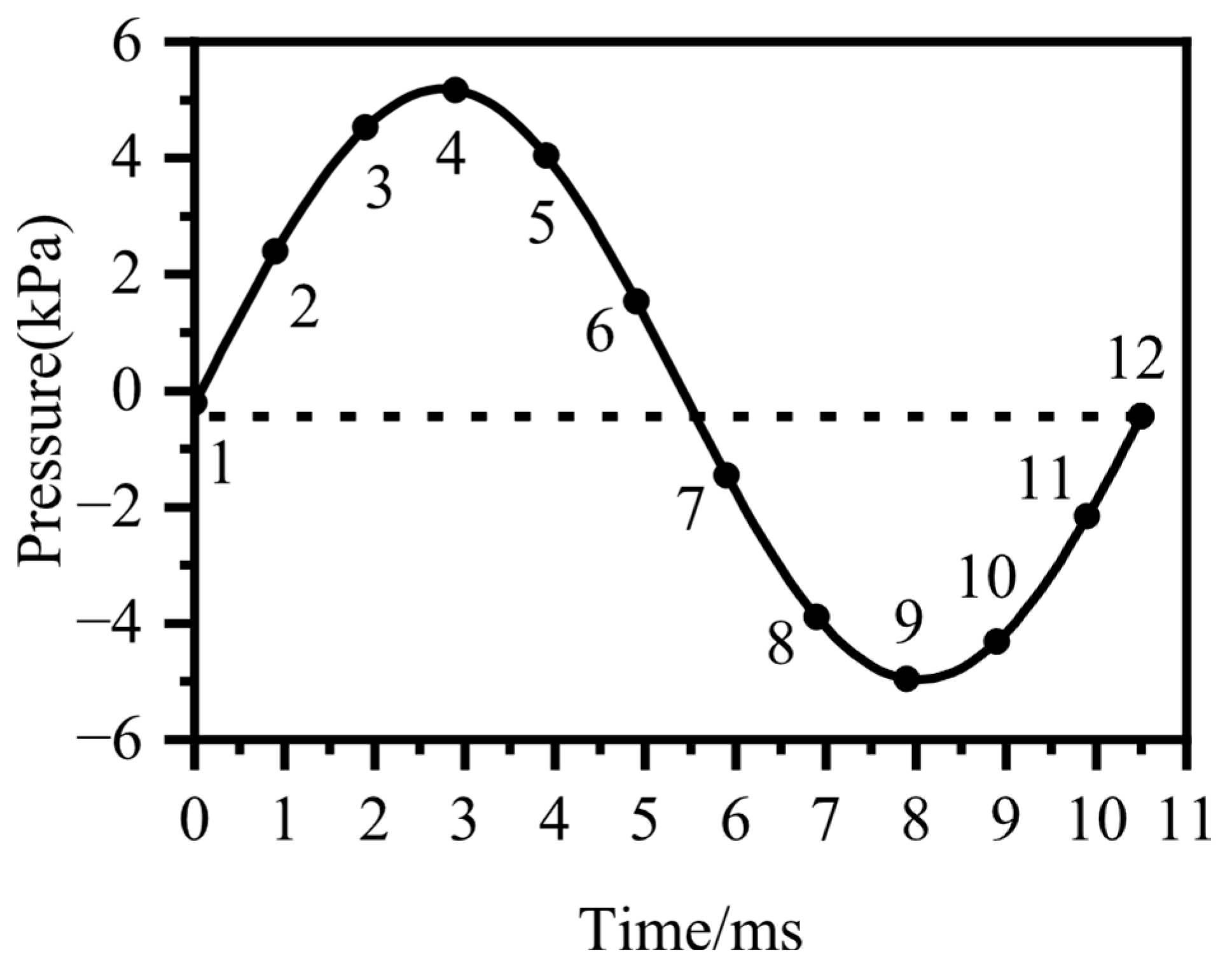
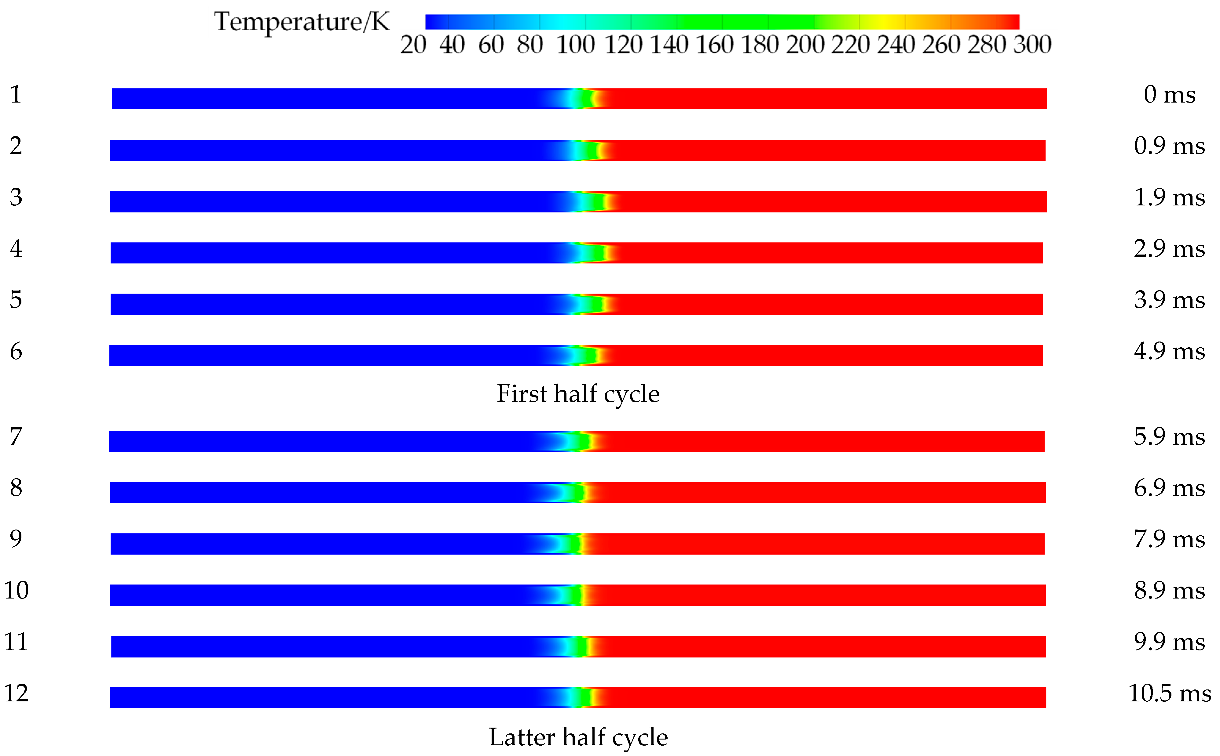
• During the oscillation process, the temperature distribution and flow characteristics of the gas inside the pipeline exhibit significant periodic changes. The cold-end gas moves towards the end of the pipeline during the first half of the oscillation cycle. Due to its low viscosity, the cold gas is easily heated and rapidly expands. In the second half of the oscillation cycle, the expanding cold gas pushes the hot-end gas to move towards the cold end, forming a low-pressure zone, which in turn triggers the reverse flow of gas. This process is constantly repeated, leading to gas oscillation.
• Under the operating conditions described in this article, thermoacoustic oscillations can also cause additional heat leakage on the pipeline wall. The average heat flux over time flows in at 1150.1 W/m² and out at 1087.7 W/m², resulting in a net inflow heat flux of 62.4 W/m². This heat maintains the duration of thermoacoustic oscillations.
• The stability limit of the system is mainly influenced by three parameters, namely the hot- and cold-end temperature ratio α, temperature gradient β, and hot- and cold-end length ratio ξ. When the critical value is exceeded, the system will oscillate.
• In practical engineering, the thermoacoustic oscillation of low-temperature hydrogen systems can be suppressed by controlling the above parameters to reach the critical range of the non-oscillation region. In addition, reducing the temperature gradient and the temperature ratio at the hot and cold ends, as well as appropriately increasing the pipe diameter and minimizing the pipe length, can weaken the amplitude of thermoacoustic oscillations.

References

1. Guo, Y.; Lei, G.; Wang, T.; Wang, K.; Sun, D. Advances in Taconis thermoacoustic oscillations. Cryogenics 2014, 2, 64–69. [Google Scholar]
2. Sugimoto, N.; Shimizu, D. Boundary-layer theory for Taconis oscillations in a helium-filled tubes. Phys. Fluids 2008, 20, 104102. [Google Scholar]
3. Shimizu, D.; Sugimoto, N. Numerical study of thermoacoustic Taconis oscillations. J. Appl. Phys. 2010, 107, 034910. [Google Scholar]
4. Ishigaki, M.; Adachi, S.; Ishii, K. Numerical analysis of stability of thermo-acoustic oscillation in a 2D closed tube. In Proceedings of the 48th AIAA Aerospace Sciences Meeting Including the New Horizons Forum and Aerospace Exposition, Orlando, FL, USA, 4–7 January 2010. [Google Scholar]
5. Ishigaki, M.; Adachi, S.; Ishii, K. Stability of thermo-acoustic oscillation in a closed tube by numerical simulation. Fluid Dyn. Res. 2011, 43, 041403. [Google Scholar]
6. Lobanov, N.R. Investigation of thermal acoustic oscillations in a superconducting linac cryogenic system. Cryogenics 2017, 85, 15–22. [Google Scholar]
7. Guo, Y.; Lei, G.; Wang, T.; Wang, K.; Sun, D. Numerical simulation of Taconis thermoacoustic oscillation. J. Zhejiang Univ. (Eng. Ed.) 2014, 48, 327–333. [Google Scholar]
8. Jiang, W.; Huang, Y.; Zhuan, R.; Zhang, L. Trigger Conditions and Suppression Measures of Thermoacoustic Oscillations in Liquid Helium Vessels. Vac. Cryog. 2018, 24, 193–199. [Google Scholar]
9. Wang, X.; Niu, X.; Bai, F.; Zhang, J.; Chen, S. Study of thermoacoustic oscillations in half-open tubes for saturated superfluid helium. Prog. Supercond. Cryog. 2022, 24, 68–73. [Google Scholar]
10. Hu, L.; Liu, Q.; Yang, P.; Liu, Y. Identification of nonlinear characteristics of thermoacoustic oscillations in helium piping systems. Int. Commun. Heat Mass Transf. 2021, 120, 104999. [Google Scholar]
11. Hu, L.; Liu, Q.; Chen, P.; Liu, Y. Numerical study on suppression of thermoacoustic oscillation in cryogenic helium pipeline system. Cryogenics 2021, 117, 103311. [Google Scholar]
12. Xia, S.; Xie, F.; Li, Y.; Guo, W. A Numerical Study on the Settlement Characteristics of Slush Cryogenic Propellants in the Tank. J. Xi’an Jiaotong Univ. 2024, 58, 146–156. [Google Scholar]
13. Gu, Y.F.; Timmerhaus, K.D. Thermal acoustic oscillations in triple point liquid hydrogen systems. Int. J. Refrig. 1991, 14, 282–291. [Google Scholar]
14. Gu, Y.F.; Timmerhaus, K.D. Damping criteria for thermal acoustic oscillations in slush and liquid hydrogen systems. Cryogenics 1992, 32, 194–198. [Google Scholar]
15. Matveev, K.; Leachman, J. Thermoacoustic Modeling of Cryogenic Hydrogen. Energies 2024, 17, 2884. [Google Scholar] [CrossRef]
16. Shenton, M.; Leachman, J.; Matveev, K. Investigating Taconis oscillations in a U-shaped tube with hydrogen and helium. Cryogenics 2024, 143, 103940. [Google Scholar]
17. Sun, D.; Wang, K.; Guo, Y.; Zhang, J.; Xu, Y.; Zou, J.; Zhang, X. CFD study on Taconis thermoacoustic oscillation with cryogenic hydrogen as working gas. Cryogenics 2016, 75, 38–46. [Google Scholar]
18. Gu, Y.F.; Timmerhaus, K.D. Experimental Verification of Stability Characteristics for Thermal Acoustic Oscillations in a Liquid Helium System. In Advances in Cryogenic Engineering; Kittel, P., Ed.; Springer: Boston, MA, USA, 1994; Volume 39, pp. 1733–1740. [Google Scholar]
Figure 1. The diagram of the simulation model used in this article.
Cryo 01 00009 g001
Figure 2. Characteristics of the initial temperature distribution curve.
Cryo 01 00009 g002
Figure 3. (a) Verification of grid independence. (b) Verification of time step independence.
Cryo 01 00009 g003
Figure 4. (a) Qualitative verification of hydrogen working fluid. (b) Qualitative verification of helium working fluid.
Cryo 01 00009 g004
Figure 5. Quantitative verification of CFD and DeltaEC results.
Cryo 01 00009 g005
Figure 6. Complete oscillation generation process.
Cryo 01 00009 g006
Figure 7. (a) Amplitude–frequency characteristic. (b) Time–frequency characteristic.
Cryo 01 00009 g007
Figure 8. Division of periodic pressure oscillation stages.
Cryo 01 00009 g008
Figure 9. Temperature changes in fluid and pipe wall in one cycle.
Cryo 01 00009 g009
Figure 10. (a) Heat flux density in the front section of the pipeline. (b) Heat flux density in the rear section of the pipeline. (c) Heat flux density in the middle section of the pipeline.
Cryo 01 00009 g010
Figure 11. (a) The influence of α on amplitude and frequency. (b) The influence of β on amplitude and frequency.
Cryo 01 00009 g011
Figure 12. The influence of the length ratio of hot and cold ends on amplitude and frequency.
Cryo 01 00009 g012
Figure 13. (a) The influence of pipe diameter on amplitude and frequency. (b) The influence of pipe length on amplitude and frequency.
Cryo 01 00009 g013
Disclaimer/Publisher’s Note: The statements, opinions and data contained in all publications are solely those of the individual author(s) and contributor(s) and not of MDPI and/or the editor(s). MDPI and/or the editor(s) disclaim responsibility for any injury to people or property resulting from any ideas, methods, instructions or products referred to in the content.