Bayesian Evidence Synthesis to Infer Unobserved Population Dynamics: An Application to International Migration Into the United States, 2000–2019

Abstract

For the United States, detailed estimates of the number of resident migrants and the rates of migrant arrival are valuable for understanding population dynamics and for determining the impact of economic and political changes that influence migration. The goal of this analysis was to derive estimates of the U.S. foreign-born population and how this population has changed in recent years, as well as estimates of recent and historical immigration volumes. Using data from large population surveys (the 2000 U.S. decennial census and 2001–2019 American Community Survey (ACS)), a Bayesian evidence synthesis was conducted to pool survey data across years while accounting for various biases and logical constraints that apply to these data. This analysis produced highly disaggregated estimates of the foreign-born population residing in the United States over the period 2000–2019, as well as estimates of immigration volume for 1950–2019. These population estimates demonstrated high in- and out-of-sample predictive performance, with substantially greater precision than that for raw survey estimates. Estimated immigration flows tracked other available time series, although with higher precision and with the potential to include undocumented immigration not represented in other immigration data. This study documents immigration from 100 countries of origin into the United States and demonstrates how the results of repeated cross-sectional population surveys can be used to infer migration dynamics that are difficult to measure directly.

1. Introduction

For high-income countries, international migration can represent an important contributor to population growth and a substantial share of the resident population. Changes in migration rates have accompanied changes in the economic and political environment in the destination country and migrants’ countries of origin, as well as changes in immigration policy [1,2,3]. The United States represents the most common destination country for migrants globally, with the U.S. foreign-born population representing 18% of global migrant stocks, more than three times greater than that in any other single country [4]. In 2023, 48 million foreign-born individuals resided in the United States, representing 14% of the U.S. population. Of this 48 million, 26 million are estimated to have entered the country since the turn of the century, while 16 million have entered since 2010, reflecting major migrant inflows over recent years [5]. These individuals play important roles across multiple domains of economic and civic life in the United States [6]. While immigration is an established feature of U.S. population dynamics, overall rates of immigration have changed substantially over time, and the mix of countries and world regions represented in successive immigration cohorts has also varied. In the early part of the 20th century, migrants to the United States were primarily from European countries. This pattern evolved with increasing migration from Asian and Latin American countries in more recent years, with individuals from these regions representing 42% and 39% of all new U.S. residents entering the country after 2010, respectively [5,7]. For some countries, migration to the United States has followed sharp changes driven by U.S. foreign policy, exemplified by the successive waves of immigration from Vietnam starting in the 1970s in the wake of the Vietnam War, which was preceded by low rates of immigration from this country [8]. The question of how migrants impact U.S. society has been the subject of substantial academic and public discourse historically [9,10], as well as more recently [11], and evidence on the changing composition of the U.S. foreign-born population is a critical input for these discussions.

For countries that receive substantial numbers of migrants, detailed estimates of the sizes and trends in the foreign-born resident population have many potential applications, including planning the provision of services for these individuals, gauging the impact of immigration policy, and generating evidence on other determinants of migration. For the United States, tabulations of foreign-born population stocks are routinely provided by the U.S. Census Bureau. However, these estimates may not stratify results according to all the dimensions that may be important for decision-making, or may be reported in categories that are overly broad for a particular use. Public-use microdata are also available for many of the large population surveys conducted in the United States, but while these datasets allow a high level of disaggregation, the sampling uncertainty associated with ‘raw’ estimates calculated directly from these data can be substantial [12]. Moreover, evidence on foreign-born immigration flows is substantially weaker than evidence on current stocks, with direct estimates of individuals legally admitted to the United States [13] excluding undocumented migrants, and indirect estimates back-calculated from the time series of population stocks affected by uncertainty around emigration volume.

The best current data on the foreign-born resident population come from the American Community Survey (ACS), which collects data on a large population-based sample of the U.S. resident population on an ongoing basis, with annual data releases [14]. The ACS collects a range of socio-economic and demographic data on sampled individuals, including information on ancestry, family relationships, citizenship status, education, languages spoken, present and past locations of residence, selected disabilities, employment, income, and household characteristics. The content and wording of these surveys closely match variables previously collected on the ‘long form’ of the decennial U.S. census, which the ACS has largely replaced. For the ACS, the foreign-born population includes legal immigrants (‘green-card’ holders), legal non-immigrants (temporary migrants), asylees and refugees, and undocumented migrants as long as they meet survey criteria for current residence. Early variants of the ACS were introduced from 2000 to 2004, and the survey has been conducted in a standardized format since 2005. For the year 2000, the 5% sample of the decennial census provides similar information on country of origin and other basic demographic data.

Despite the large sample size of the ACS, there is substantial sampling uncertainty for detailed population estimates. The errors induced by this sampling uncertainty can be revealed by following a single immigration cohort over time. While population estimates for an immigration cohort should decline over time (as individuals exit the cohort due to death or emigration), the raw data show periods of apparently increasing populations. For example, the raw population estimate for the 2000 entry cohort from the Philippines (the country of origin with the fourth largest number of U.S. residents in the 2019 ACS) increased from 38,000 to 49,000 between 2001 and 2002 and from 46,000 to 59,000 between 2016 and 2017. Between 2001 and 2019, 10 of 18 years featured apparent population increases despite this being a closed cohort. These estimation errors are proportionally larger for countries with smaller resident populations and are also seen with other population attributes—for example, in the 2000 entry cohort from Moldova, the average age from the raw survey data declined from 50 years old in 2006 to 26 years old in 2007 before rising to 37 years old the next year.

In addition to random variation, there are also systematic artifacts apparent in ACS survey responses. For example, reported years of entry show periodic spikes, with foreign-born respondents being 34% more likely to report entering in the first year of the decade (1960, 1970, 1980, 1990, 2000, or 2010) than in the years immediately before or afterwards. Similar but smaller spikes are observed for ‘half-decade’ years (1955, 1965, etc.), with respondents being 14% more likely to report entering the United States in these years than in the years immediately before or afterwards. It is difficult to explain these periodic spikes as resulting from real immigration trends, and they are more likely caused by some bias in terms of how the year of entry is reported or recorded. The magnitude of these spikes makes it difficult to distinguish real changes in immigration volume from the reporting artifacts in the raw data.

The objective of this analysis was to propose a novel approach for generating estimates of the number of foreign-born individuals living in the United States, simultaneously stratified by several dimensions to provide high-precision estimates of the U.S. foreign-population for a large number of population strata, while minimizing sampling uncertainty and adjusting for reporting biases associated with available survey data. This analysis was additionally designed to produce estimates of migration into the United States by country, year, and age for the period covered by survey data, as well as past years. To achieve these objectives, this study combined 20 years of survey data with a mechanistic model of foreign-born population dynamics. In this model, each immigration cohort (by country, entry year, and age) was followed over time, with mortality rates based on published lifetables and emigration rates estimated from the survey data. As a result, the population of each immigration cohort was allowed to decline over time based on established components of population changes. By placing logical and probabilistic constraints on how individuals enter and exit the foreign-born population, the analytic approach was able to reduce the sampling uncertainty associated with the survey estimates and adjust for sources of bias in these data.

The results of this study represent precise estimates of the number of foreign-born individuals living in the United States for calendar years 2000–2019 stratified by multiple individual-level characteristics (country of origin, year of age, year of entry to the US, and calendar year). The analysis also provides annual estimates of foreign-born individuals newly entering the U.S. resident population, a measure of annual immigration volume that may have advantages compared to other approaches. This paper describes the statistical approach used to model population changes and generate results, reports tests of in- and out-of-sample predictive performance, provides the population estimates, and highlights applications for these estimates. While the focus of this study was the United States foreign-born population, the approaches developed through this study may be applicable to other countries that collect cross-sectional population data though large surveys or administrative records.

2. Materials and Methods

2.1. Data

The primary data source used for this analysis was the America Community Survey (ACS). We used ACS public-use microdata samples (PUMS) from surveys conducted from 2001 to 2019. We also used the 5% sample of the 2000 decennial census, which represents 5% of all eligible individuals. PUMS data are created from original survey responses, with edits made to impute missing, illegible, or illogical values and to prevent identification of survey respondents [15]. ‘Foreign-born’ individuals were defined as survey respondents reporting a place of birth outside of the U.S. or U.S. territories, excluding individuals born to U.S. parents. To be a U.S. resident (and therefore be included in the ASC survey sample), an individual must have lived at their U.S. address for >2 months or anticipate living at that address for >2 months. Variables for place of birth, year of U.S. entry, and current age were extracted from survey data, in addition to analysis weights provided to inflate the individual samples to obtain national population estimates. The sum of these analysis weights was taken to represent the ‘raw’ population estimate for any given stratum.

The variable for year of entry into the United States showed irregular patterns for entry years prior to 1950 resulting from census statistical disclosure controls, and this variable was therefore bottom-coded at 1949. Similarly, the variable for current age showed irregular patterns for advanced ages and was thus top-coded at 91. ISO 3166-1 alpha-3 codes (ISO3 codes) were used to identify countries. Individuals were assigned to a single ISO3 code according to their survey country-of-origin code. For survey country-of-origin codes describing a dependent territory without an ISO3 code, individuals were assigned to the governing state of the territory. All other individuals that could not be mapped to a unique ISO3 code were pooled into a residual category. In addition, countries becoming independent states after 2000 (Kosovo, Montenegro, Serbia, South Sudan, and Timor–Leste) were pooled with the state they were part of as of 2000 (Yugoslavia, Sudan, and Indonesia). Using the country-of-origin variable, an additional classification was created to group individuals into world region of origin using the World Bank regional classification (East Asia and Pacific, Europe and Central Asia, Latin America and the Caribbean, Middle East and North Africa, North America, South Asia, and Sub-Saharan Africa). Using these classifications, a combined dataset of raw survey estimates was created from the individual-level PUMS data for all possible combinations of country or region of origin, current age, year of entry, and survey year.

2.2. Analysis

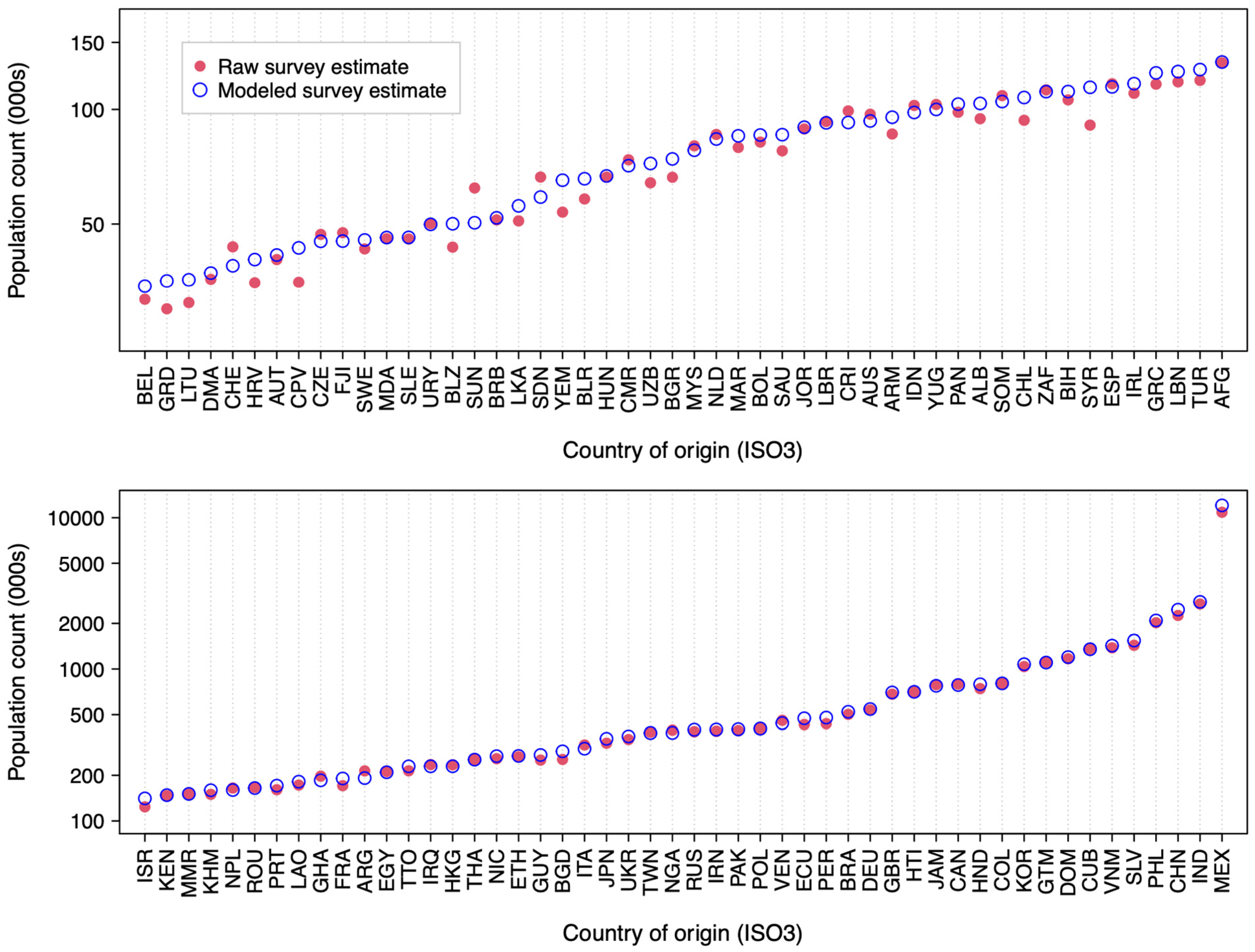
Analyses were undertaken to obtain population estimates for the U.S. foreign-born population stratified by country or region of origin, current age, year of entry, and survey year. These included 76,830 unique values for each country or region of origin. Results were estimated for the overall foreign-born population, for each world region of origin, and for each of the top 100 countries of origin (ranked according to U.S. resident population size for each country of origin, averaged over the period 2000–2019).

2.2.1. Immigration Cohort Model

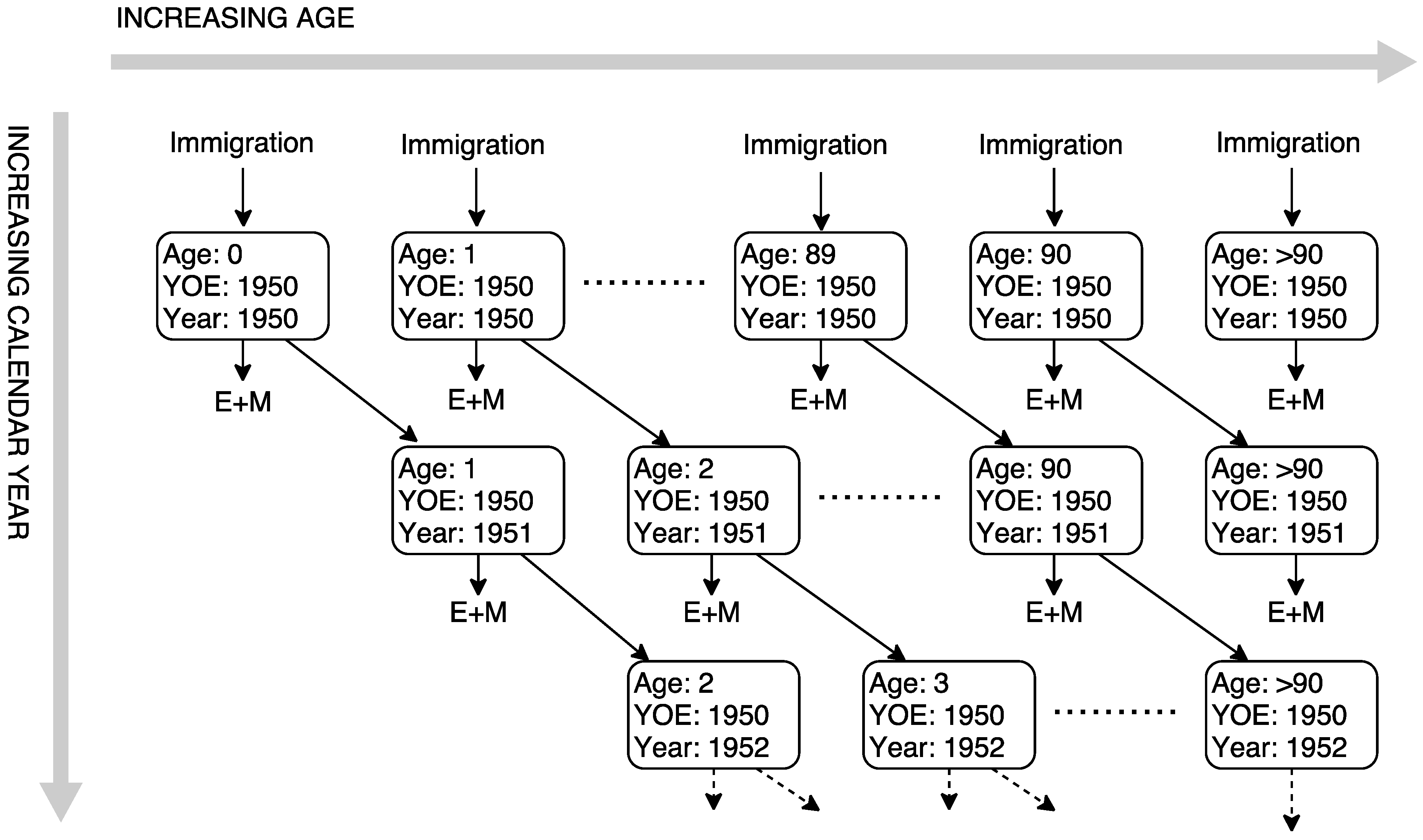
A compartmental stock–flow model was developed to represent the population dynamics of the foreign-born U.S. population from 1950 to 2019. This model allowed (i) an existing stock of foreign-born individuals in 1950, (ii) yearly additions to the foreign-born population in each year from 1950 to 2019 due to immigration, and (iii) yearly exits from the foreign-born population due to emigration or death. In this model, individuals residing in the United States in a given calendar year were stratified by year of age and entry year. The number of individuals in a particular immigration cohort (defined by year and age of entry) present in the United States in a given year was assumed to be equal to the number of individuals in the same immigration cohort in the previous year minus exits to emigration or death. Figure 1 shows a schematic of this stock–flow model for the 1950 immigration cohort.

2.2.2. Initial Population

The initial population for the model was composed of all foreign-born individuals present in the United States at the start of 1950 stratified by age. Data for cohorts immigrating to the United States before 1950 were combined into a single cohort, as this group represents a small fraction of the current foreign-born population (approximately 1%).

2.2.3. Immigration

The total immigration volume each year from 1950 to 2019 was modeled as a geometric random walk, and the age distribution of immigrating cohorts was represented using penalized B-splines [16,17]. This age distribution consisted of the following two components: a one-dimensional spline representing the average age distribution across all entry years and a two-dimensional spline surface representing temporal deviations from this average pattern.

2.2.4. Emigration and Mortality

Individuals exited the resident foreign-born population through mortality and emigration. Evidence on mortality rates by single year of age was drawn from recent U.S. life tables [18]. Variation in these age-based mortality rates was modeled via a penalized B-spline to allow for deviations in mortality rates between the general population and individual immigrant groups. In addition, age-specific mortality rates were assumed to decline log-linearly over time based on trends reported in decennial life tables for 1950–2010 [18].

Exits due to emigration were assumed to decline with increasing time since entry [19,20], with the emigration rate allowed to decline smoothly up to 15 years after entry to the US, after which it was held fixed.

2.2.5. Misclassification of Reported Age and Entry Year

Population estimates calculated directly from the survey data showed periodic spikes in the population distribution as a function of reported age and entry year (Supplementary Materials, Figure S4). For both of these variables, large spikes were apparent, coinciding with the end of each decade, and smaller spikes were apparent at mid-decades. In other studies, implausible patterns in ACS results have revealed systematic biases due to misreporting by survey respondents [21,22], and it was hypothesized that the periodic effects observed in the raw estimates resulted from misreporting by survey respondents, with the true value for age and/or entry year being rounded to the nearest decade or mid-decade. A measurement–error model was used to correct for this misclassification.

2.2.6. Undercounting of Foreign-Born Populations

Previous research suggests that raw estimates derived from the ACS underestimate true population sizes for foreign-born populations [23]. While analysis weights provided for the ACS are adjusted to account for under- or over-reporting, the ACS is only controlled by age, sex, race, and Hispanic origin, not nativity. The extent of undercounting is thought to be greater for recent immigrants, undocumented migrants, immigrants of Hispanic origin, younger age groups, and older ACS survey years [23,24,25]. The magnitude of this bias cannot be estimated from the survey data alone, and evidence of undercounting is generally derived from comparison with other data sources. Using estimates of the size of the ACS undercount reported by the U.S. Census Bureau [23], the analysis allowed for underreporting in the PUMS data so that final analytic estimates would provide an estimate of the true population size. These adjustments were specified as inflation factors that varied with time since entry (higher for more recent immigrants), country of origin (higher for countries in Latin America and the Caribbean), and survey year (higher for earlier survey years with smaller sample sizes). For countries in Latin America and the Caribbean, an average undercount rate of 5.0% was assumed for survey years 2005–2019, and an average undercount of 2.0% was assumed for other countries over the same period, consistent with recent Census Bureau estimates [23].

2.3. Estimation

A Bayesian approach was used to implement the analysis. First, formulae describing the relationship between model parameters and population totals were defined, and a likelihood function was constructed for the survey data. In these likelihoods, the raw population estimates were calculated as the sum of analytic weights for each stratum in the analysis. Second, probability distributions were defined for each model parameter. In general, weakly informative priors [26] were specified, except where substantial prior information was available, such as with age-specific population mortality rates. Final parameter values were estimated as the product of the prior distribution and the likelihood function, following conventional Bayesian approaches. These fitted parameter values were used to calculate the population estimates. The analysis was conducted separately for each country and region of origin.

Model estimates for the surveyed population (reflecting any misreporting and underreporting) were compared to the raw survey values to validate the estimation results (next section). For each country or region of origin, ‘true’ values were also produced, which were adjusted to remove the effects of misreporting and underreporting. In addition to these population estimates, the analysis produced estimates of annual entries to the population covered by the ACS and census as a measure of immigration volume.

Data processing was conducted in R v4.0.2 [27], and the model was fitted using adaptive Hamiltonian Monte Carlo sampling, as implemented by the Stan probabilistic programming software v2.21.2 [28,29]. The sampler was run with 3 chains of 2000 iterations each. Each country was fit separately, and the first 1000 draws were discarded as warm-up values. The remaining samples were thinned to retain every 5th draw, producing a posterior sample of 600 parameter sets for each country. The mean of these posterior samples was used to create point estimates for each population group of interest, and equal-tailed 95% uncertainty intervals were calculated to quantify uncertainty in estimates. Full details of the technical specification of this analysis, including model equations, prior distributions, and likelihood function, are provided in the Supplementary Materials.

2.4. Cross-Validation

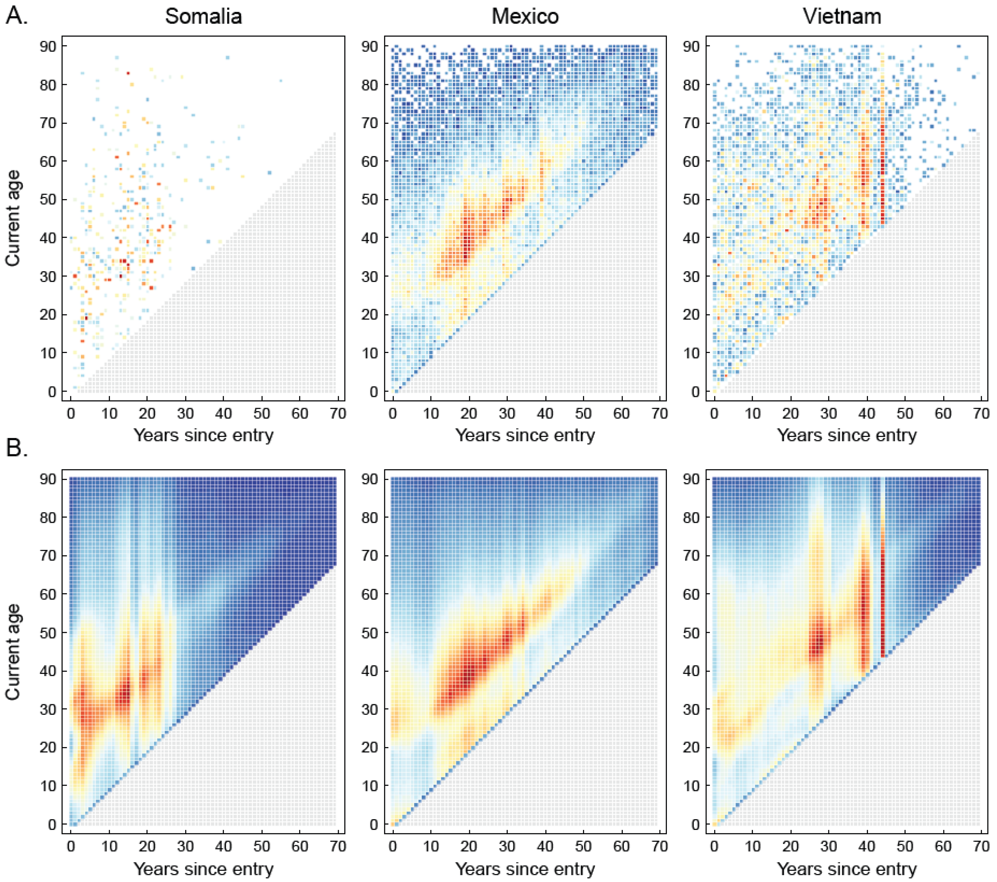
To validate the estimation approach, how well the model could predict data not used for model fitting (“out-of-sample predictive performance”) was assessed [30,31]. To do so, the model was re-estimated for a sample of seven countries with selected survey years removed, testing the ability of the estimation procedure to reproduce the population estimates for the held-out survey years. 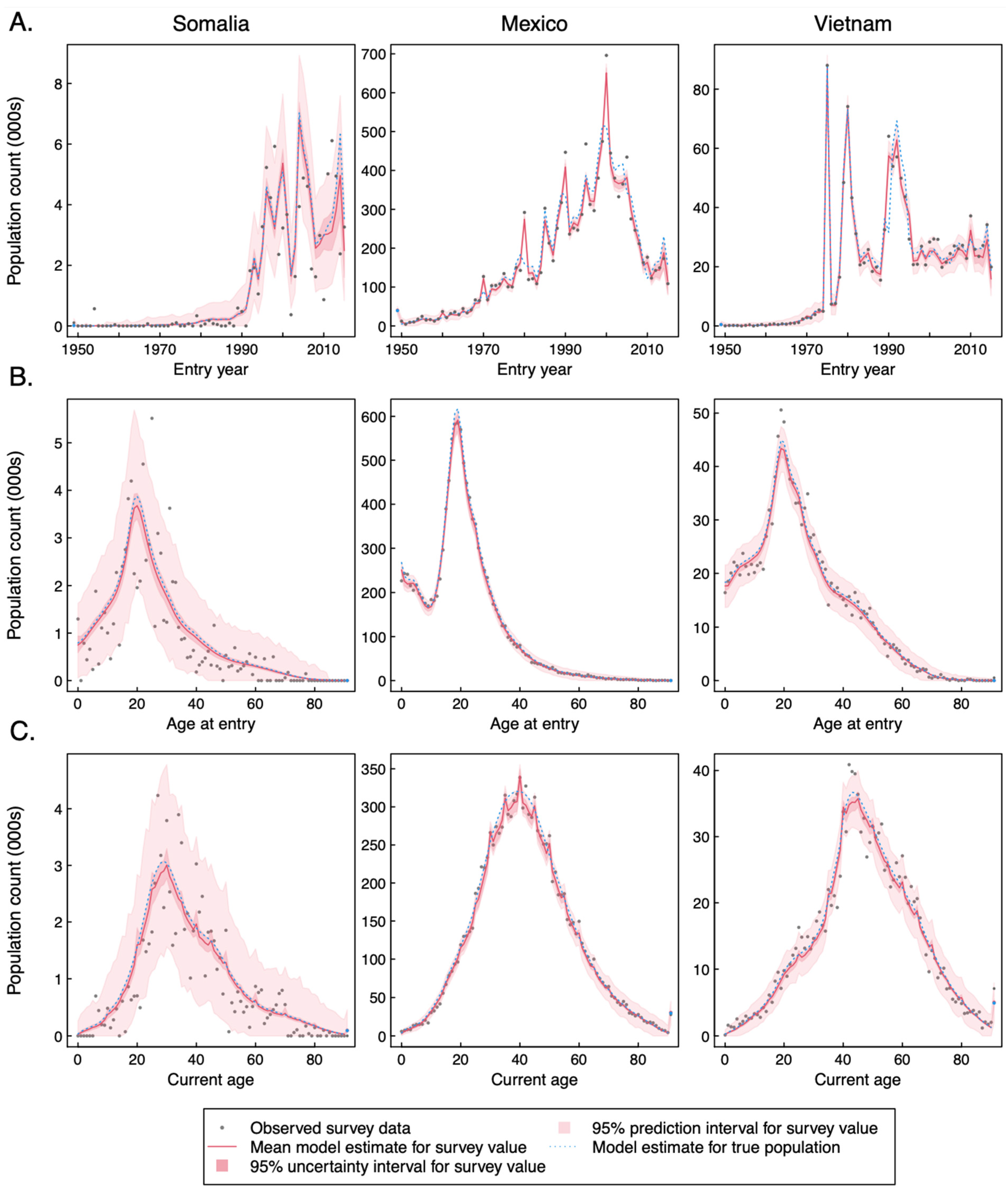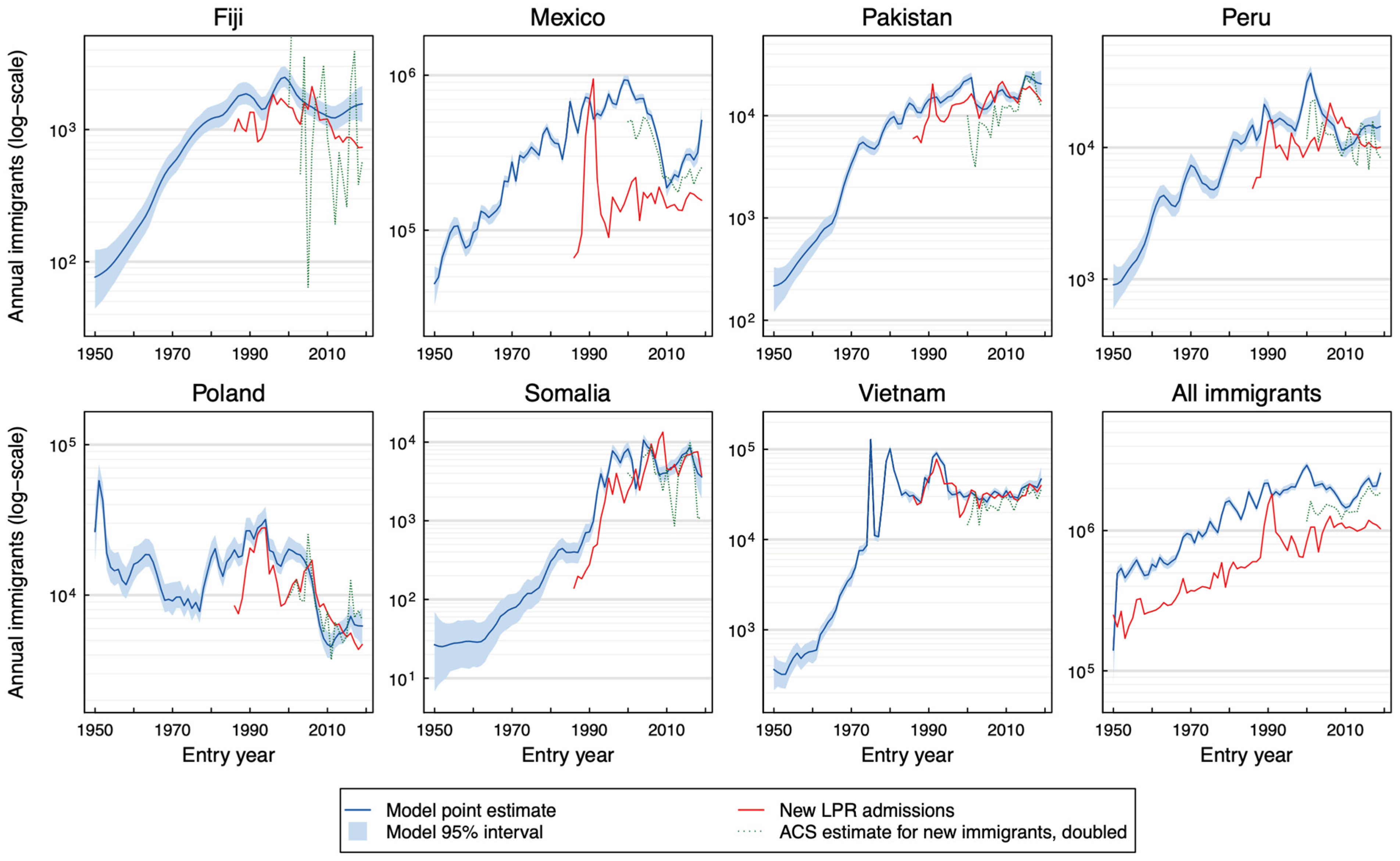This block cross-validation approach was adopted to provide a more rigorous test of predictive performance (as compared to assessing predictive performance in randomly chosen hold-out samples), giving the potential for non-independence of population data within each survey year [32,33]. The countries used for this validation exercise—Fiji, Mexico, Pakistan, Peru, Poland, Somalia, and Vietnam—were chosen to represent a range of world regions and resident population sizes, which may present different estimation challenges. For each of these countries, the model was re-estimated three times, holding out data for the years 2005, 2010, and 2015, and fitting the model to the remaining data. These models were refit a fourth time, holding out data for the last two survey years (2018–2019) to assess the ability of the estimation approach to predict future population values.

Results from these analyses were compared to the data from survey years not used for model fitting to assess out-of-sample predictive performance. Estimated values and held-out survey data were compared visually, plotting the estimated population as a function of each dimension of interest (year of entry, age at entry, and current age) in order to identify systematic deviations that might suggest a problem with the estimation approach. In addition, standardized residuals were calculated by dividing the estimation residuals (raw survey estimate for a unique combination of place of birth, year of entry, and current age minus the modeled estimate for the same value) by the standard error estimates provided by the survey methodology [34]. Theoretically, these standardized residuals would have a standard deviation of 1.0 for a model that perfectly predicted the mean of each observation. The fraction of instances in which the survey estimate was predicted to be zero (i.e., no individuals with a given set of characteristics included in the sample) was also calculated and then compared to the empirical distribution from the survey. With a well-performing model, the modeled probabilities should reproduce the observed frequencies. Finally, logged values for modeled vs. raw population estimates were plotted to assess any estimation errors associated with the magnitude of population estimates. With a well-performing model, the points on these scatterplots should cluster on the diagonal. The out-of-sample predictions were also compared to the estimates obtained in the main analysis using rank correlation and the mean absolute difference (calculated as a percentage of the main analysis value) to characterize the differences between the two sets of estimates.

Two additional tests of validity were performed. Firstly, the model was re-estimated having excluded all data for survey years 2001 to 2005 for each of the seven test countries described above (Fiji, Mexico, Pakistan, Peru, Poland, Somalia, and Vietnam). Before 2006, the ACS samples were substantially smaller than the final size (approximately 1% of the U.S. population) and excluded individuals in group quarters. Including the data from these earlier ACS rounds provided additional information for the analysis, although doing so could potentially bias the results due to the different populations covered by the pre-2006 ACS rounds compared to later rounds. The results for 2001–2005 from this analysis were compared to those obtained in the main analysis, quantifying the agreement between these estimates using rank correlation and the mean absolute difference. Secondly, the model was re-estimated using a dataset that excluded individuals with imputed values for at least one of the variables used in the analysis. This imputation is performed by the U.S. Census Bureau when an individual’s response on a given survey question is missing or illegible or has inconsistent values. While this imputation facilitates data analysis, systematic errors in the imputation approach could lead to biased inference. To implement this sensitivity analysis, a new dataset was created that excluded individuals with imputed variables, and then the analytic weights were inflated by a constant proportion to match the original population estimate for each survey year. Using these adjusted datasets, population estimates were calculated for each of the seven test countries (Fiji, Mexico, Pakistan, Peru, Poland, Somalia, and Vietnam). These estimates were compared to those obtained in the main analysis, with differences quantified using rank correlation and the mean absolute difference.

3. Results

3.1. Comparison of Modeled Results to Raw Survey Estimates

Figure 2 shows the total population estimates for 2019, comparing modeled estimates for the true population (i.e., controlling for undercounting and misclassification of demographic data by survey respondents) to ‘raw’ survey estimates, which were estimates derived directly from the PUMS data by weighting observations by the analysis weights provided. As might be expected, the modeled population estimates for countries of origin with large resident populations (Figure 2, lower panel) were very similar to the raw survey estimates, as for these populations, the raw estimates had low sampling uncertainty relative to the size of the population. For countries of origin with smaller resident populations (Figure 2, upper panel), there were more substantial differences between modeled and raw estimates, reflecting greater sampling uncertainty in the results of an individual ACS round. As an example, population estimates for immigrants from Switzerland had a noticeable difference between modeled and raw population estimates for 2019 (raw estimate = 43,600, modeled estimate = 38,800 [95% uncertainty interval 37,900; 39,800]). Compared to the average population estimate from the three prior survey years, the raw 2019 population estimate for Switzerland was 23% higher, with an increase of 9700 compared to that the year before. While this could signal a major uptick in new immigrants compared to death and emigration, the number of individuals from Switzerland in their first year in the United States was only 1500 in the 2019 ACS, implying a much lower immigration rate than would be needed to explain this result. This suggests that the high 2019 population estimate for Switzerland is simply a consequence of sampling uncertainty. The modeled estimate, by incorporating evidence across the 20 survey years, was robust to sampling uncertainty in individual survey years. This effect of smoothing implausible deviations in the time trend resulted in a lower modeled population estimate for 2019, with essentially no change in the population total (a 0.4% (−0.3, 0.9) decrease) compared to the modeled estimate for the preceding year. Figures comparing the time series of modeled population estimates to raw survey values for 2000–2019 are provided in the Supplementary Materials. The Supplementary Materials also include figures comparing modeled to raw estimates for the 2019 resident population distributed by current age, age at entry, and year of entry (Figure S9).

While the modeled estimates appear to have some advantages for estimating total population sizes for countries with smaller resident populations, the utility of these estimates is more obvious when comparing estimates for more highly disaggregated population strata.

Figure 3 compares modeled and raw 2019 population estimates for three countries (Somalia, Mexico, and Vietnam) stratified by single year of age and single year of entry. Panel A shows heatmaps of population density created from raw survey values, where the effects of sampling uncertainty can be seen. In this figure, each cell represents a single population stratum (defined by year of age and years since entry), and warmer colors indicate greater populations within that stratum. An empty cell indicates that no one from that stratum was included in the ACS survey for that year. Even for Mexico—the country of origin with by far the largest resident population—there are multiple strata where no individuals were included in the survey, and sampling uncertainty can be observed in the variation in color between adjacent cells. Vietnam has a smaller resident population, and while major features of the population distribution can be seen, there is substantial noise apparent in the raw values. For Somalia—a country whose resident population is less than 1% of Mexico’s—there is little that can be learned from the raw survey values, with the majority of strata being empty. Panel B shows heatmaps of population density created from the modeled estimates. By incorporating evidence from across the 20 survey years, these modeled estimates provide lower variance estimates of the population distribution, demonstrating patterns that could be difficult to observe in the raw values.

There are alternative approaches that could reduce sampling uncertainty in these small-group estimates. In particular, more precise estimates could be obtained by pooling categories of interest together [35] and therefore using a coarser grid to stratify the population, such as by using 5- or 10-year-wide bins for age and years since entry. However, such coarsening could obscure relevant features of the distribution, such as the spike in the population from Vietnam reporting 41 years since entry. This corresponds to an entry year of 1975, with over 10 times the number of individuals estimated to share this entry year in 2019 compared to 1974 or 1976. Using wider bands to categorize age and years since entry would not fully obscure such a major immigration cohort, but potentially useful information would be lost. Population estimates for these highly disaggregated population strata, for calendar years 2000 to 2019 and for each country or region of origin, are included in the Supplementary Materials.

3.2. Validation and Sensitivity Analyses

Out-of-sample predictive performance was used to assess the validity of the estimation approach. Figure 4 compares modeled and raw 2015 population estimates for three example countries (Somalia, Mexico, and Vietnam). For each country, estimates were produced by a model fitted to the time series of data excluding 2015. Two sets of modeled estimates are shown—estimates of the ‘true’ resident population (dashed blue lines), which were adjusted for biases introduced by misreporting of demographic characteristics by survey participants, as well as under-coverage of the ACS, and estimates of the survey population (solid lines and shaded regions), which were not adjusted for these effects and are therefore directly comparable to raw survey results. These figures show the modeled estimates closely following the systematic patterns apparent in the raw survey estimates (points). The prediction intervals, which should contain approximately 95% of the survey estimates if the estimation approach performs correctly, also appear to be well calibrated. In the Supplementary Materials (Figure S7), similar comparisons are shown for seven countries (Fiji, Mexico, Pakistan, Peru, Poland, Somalia, and Vietnam) and each of the three hold-out years (2005, 2010, and 2015).

In addition to comparing out-of-sample performance graphically, standardized residuals were calculated to quantify differences between raw and modeled population estimates. Across the 21 country–year comparisons considered in the out-of-sample validation, the standard deviation of these standardized residuals ranged from 0.23 to 1.67, with a mean value of 1.09. These standard deviations falling below 1.0 (theoretically optimal predictive performance) would normally imply over-fitting of the observed data, yet this is not possible as the validation data were not used to fit the models. Values lower than 1.0 were only observed for countries with small resident populations (Fiji and Somalia), and therefore, the most likely explanation for this finding is that the method provided by the ACS to calculate standard errors is conservative in the context of small population counts. Similarly, other approaches used to assess model performance (log–log scatterplots of modeled vs. raw population estimates, comparison of modeled vs. predicted probabilities of an individual is a given stratum being included in the survey) did not reveal any major problems with the estimation approach (Supplementary Materials, Figure S7). When the out-of-sample predictions were compared to the estimates from the main analysis, the rank correlation was found to be >0.999 for each of the 21 country–year comparisons. The mean absolute difference (calculated as a percentage of the value obtained in the main analysis) varied from 0.9% to 4.7%, with a mean of 2.1%.

Out-of-sample predictive performance was somewhat worse when data for 2018 and 2019 (the most recent 2 years of data) were excluded from model fitting (Supplementary Materials, Figure S8). While the standardized residuals were relatively similar (standard deviations ranging from 0.25 to 2.16, with a mean value of 1.22), the rank correlation with estimates from the main analysis was lower (range 0.992–0.998), and the mean absolute difference varied from 3.3% to 17.7%, with a mean of 6.5%. This reduction in predictive performance was primarily observed in the estimates for the cohorts entering the United States during the hold-out years (2018–19), for which the mean absolute difference ranged from 15.2% to 221% (average 60.8%) across the 14 country–year comparisons.

As an additional test of validity, the model was re-estimated having excluded all data for survey years 2001 to 2005 for each of the seven test countries and then used to predict values for the excluded years. For each of the 35 country–year combinations in this comparison, the rank correlation between the two sets of estimates was consistently above 0.997, and the mean absolute difference ranged from 2.4% to 8.8% of the population estimate from the main analysis (average 5.0%).

As a final sensitivity analysis, the model was re-estimated using a dataset that excluded individuals with imputed or edited data (15.1% of all observations). Using this approach, population estimates were calculated for each of the seven test countries. For each of the 140 country–year combinations in this comparison, the rank correlation between the two sets of estimates was consistently above 0.98. However, the mean absolute differences ranged from 8.6% to 43.5% of the population estimate from the main analysis (average 17.4%), indicating substantial differences between the two sets of estimates in some situations. In this comparison, the mean absolute differences were highest for Somalia, and for all countries, they were lower in more recent years (ranging from 8.6% to 28.2% in 2019) than in earlier years.

3.3. Volume of Migration

With the estimation approach used, the relationship between population sizes in successive survey years was explicitly modeled via the components of population changes. In the analytic model, entries (immigration) and exits (death, emigration) from the resident foreign-born population were allowed to vary as a function of current age, years since entry, country or region of origin, and calendar year. With time-series data on total populations, the absolute entries and exits from the population totals cannot be uniquely identified, with only the year-on-year difference between these quantities known (entries and exits from the population could be increased or decreased by matching amounts for the same net change). However, using data on years since entry allows these two processes to be distinguished—by definition, individuals can only enter an immigration cohort with years since entry equal to zero, and for subsequent years (i.e., with years since entry > 0), the only change in the cohort will be through exits to death or emigration. This was exploited to derive estimates of the number of individuals newly entering the foreign-born population each year as a measure of immigration volume for each country and region of origin. By assuming that emigration rates were only influenced by current age, country or region of origin, and years since entry and that age-specific mortality rates followed a well-defined time trend, it was possible to estimate immigration totals for the full period from 1950 to the present. Figure 5 presents estimated annual immigration volumes for the seven example countries used for out-of-sample predictive checks, as well as for the total foreign-born population. As these estimates were derived from models fit to ACS data, these estimates represent the number of individuals entering the country to become a ‘resident’ according to the definitions used in the ACS (i.e., current or anticipated residence at the current address for more than two months).

The modeled immigration estimates can be compared to those from other approaches for estimating immigration flows. In addition to the modeled estimates, Figure 5 presents the numbers of new legal permanent resident (LPR) admissions per year (red line). These data are reported in a standardized format by the Department of Homeland Security Office of Immigration Statistics and are commonly used to describe immigration rates. However, using these data to make inferences about the level and trend of total immigration faces several challenges. The first of these is the potential for delays between year of entry to the country and year of obtaining LPR status, with approximately half of all LPR immigrants entering the United States several years before obtaining LPR status (termed ‘change-of-status’ LPR applications). This time lag can distort estimated immigration trends, particularly where there are events that produce fluctuations in approved ‘change-of-status’ LPR applications that are unrelated to actual immigration rates. A prominent example of this is the Simpson–Mazzoli Act of 1986, which led to a large number of previously undocumented residents gaining LPR status over a short period of time. This produced a large spike in the LPR time series around 1990–1991, which is visible for several of the countries shown in Figure 5. Another drawback of using LPR data to track immigration flows is the exclusion of undocumented migrants, as for some countries of origin, particularly those in South and Central America, a substantial fraction of migrants are thought to be undocumented. Others will enter and reside in the country legally but hold non-immigrant visas and therefore not be included in the LPR data. As the modeled estimates are based on the ACS, they will include legal immigrants (LPR), legal non-immigrants (temporary migrants), humanitarian migrants, and undocumented migrants as long as they meet survey criteria for current residence [9]. The difference between LPR immigration and the more inclusive modeled estimates can be seen most prominently in Figure 5 for Mexico and all immigrants, where the LPR time trend is substantially lower than that of the modeled estimates. For other countries, particularly Vietnam, the LPR time series and modeled estimates track each other closely.

The raw ACS estimate for individuals who reported entering the country in the same year as the survey was conducted provides another approach to estimating immigration flows (Figure 5, green line). A major challenge for this approach is the need to adjust for the fact that this population is only partially observed in the ACS—as the ACS is conducted continuously throughout the year, interviews conducted earlier in the year will exclude individuals entering the country later in the year. In Figure 5, this undercount was adjusted for by simply doubling the raw values, which would be appropriate if migrants entered the country at a constant rate throughout the year and immediately met the ACS inclusion criteria. However, it is not clear that these assumptions hold. Moreover, the raw ACS values exhibit increased variance compared to the modeled values, which is particularly apparent for smaller countries of origin like Fiji, and provide no information on immigration flows in years prior to the observed survey period.

Immigration trends were calculated for each country and region of origin, and Figure 6 reports recent immigration trends for all immigrants grouped into world regions (according to World Bank regional groupings). These results show differential trends between world regions, with progressive growth from South Asia and Sub-Saharan Africa compared to other world regions. Some systematic patterns are likely to result from geopolitical events, with immigration from all world regions declining sharply between 2000 and 2002, possibly as a result of the September 11 terrorist attacks. More recently, a major and sustained decline in immigration from the Latin America and Caribbean region occurred between 2000 and 2005, producing a greater than 50% absolute reduction in annual immigration, with this decline almost completely reversed by growth over the following 5-year period. This major decline and the subsequent rebound were not apparent for other world regions and were not seen in the LPR estimates (Figure 5), although immigration from Europe and Central Asia showed a more modest decline and recovery over the same period. By 2019, annual immigration was estimated to have reached its highest level since 1950 (and potentially highest ever), driven by migration from the Latin America and Caribbean region as well as the East Asia and Pacific region, both of which reached peak immigration rates in 2019.

4. Discussion

This paper reports highly disaggregated estimates of the foreign-born population residing in the United States for the period 2000–2019 stratified by country and region of origin, current age, and year of entry to the US. By pooling estimates across several survey years, these estimates are substantially more precise than estimates calculated directly from the raw survey data. The approach used to obtain more precise estimates—following individual immigration cohorts through the time series of survey data and assuming smooth distributions for various demographic characteristics—differs from variance reduction approaches commonly applied to these data, which involve aggregating data within larger categories [36] or across multiple survey years via the ACS 3-year and 5-year estimates. While these approaches can successfully reduce variance, they can also obscure important features of the data in those circumstances where outcomes of interest vary across the categories being aggregated. As well as providing improved precision, the modeled population estimates adjust for biases in the ACS data, including the tendency for some survey respondents to round their demographic data to the nearest decade and under-coverage of the foreign-born population, particularly in the early years of the ACS. In addition to these population estimates, estimates of new entries to the resident foreign-born population are also reported as a measure of annual immigration volume. These estimates are inclusive of undocumented and temporary migrants, populations for whom immigration and residency estimates are of substantive interest but are difficult to obtain [37,38,39,40].

The Bayesian statistical approach taken by this analysis is becoming more commonly used to produce migration estimates, allowing the synthesis of multiple evidence sources, representation of various artifacts in source data, and quantification of uncertainty in resulting estimates [41,42]. Prior applications of this approach have focused on individuals countries and regions [43,44,45] or have generated global estimates for all county–country dyads [41,42,46]. Most Bayesian applications have used regression models to pool data, with migration estimates calculated from a linear function of chosen predictors. For example, Cohen et al.’s approach to producing international migration projections for any country–country dyad fit a generalized linear model to migration data reported by 11 countries, with final estimates calculated as the product of the population of origin and destination countries, the area of the origin country, and the distance between the two counties, each raised to a power term estimated from the data [46]. In contrast, this analysis specified a mechanistic model relating migration estimates to study data. This difference stems from the data available for estimation—while these other studies used data on migration flows directly, the present study inferred migration indirectly based on cross-sectional population estimates, an approach previously used by Aparicio Castro et al. to infer migration flows between South American countries using census data [45]. As compared to other studies, the present analysis did not use data on known determinants of migration (economic and social factors, immigration policy) [1,2,3] as part of the estimation approach. While incorporating this evidence may have produced more precise estimates, it would have undermined the utility of the resulting estimates for investigating these migration determinants.

There are multiple potential uses for the detailed population estimates produced by this analysis—by improving the precision of stratified population estimates, patterns and temporal trends in these populations can be more easily observed, which may suggest directions for further investigation. Changes in the resident population for individual countries of origin are difficult to discern from the raw ACS data, particularly for countries with small resident populations, yet these trends can be reported directly from the new estimates. Similarly, changes in age distribution can also be reported with greater precision using the new estimates. These outcomes are useful for describing the changing composition of the foreign-born population residing in the United States. Similarly, the results for immigration volume have multiple applications for understanding who is entering the United States to live and how this has changed over time. In particular, by comparing the immigration flows estimated by this analysis to reported data on rates of legal migration [13], it is possible to estimate migration rates for undocumented individuals, extending approaches developed in other analyses to estimate current population volumes for undocumented individuals [37,47,48].

In addition to describing patterns and trends, the disaggregated population estimates can also be used as inputs into other analyses. The initial motivation for this study was to obtain population denominators for an epidemiological assessment of infectious disease burden in the foreign-born U.S. population [49], where it was expected that disease burden would likely differ according to several of the demographic characteristics considered in this study. It is likely that other analyses would also benefit from fine-grained data on population distributions for this group, providing population denominators with which measures of the incidence or prevalence of a condition of interest can be calculated [50,51,52]. Similarly, estimates of immigration rates can provide inputs into analyses that seek to identify the underlying causes of changing migration rates [53,54,55], or that investigate how immigration has influenced other outcomes within the United States [56,57]. Finally, by investigating situations when model fit to data is poorer than predicted by sampling uncertainty, it could be possible to identify reporting artifacts or biases affecting how current data are being interpreted, which could allow progressive improvements to survey approaches. Apart from the estimates themselves, the estimation approach developed in this study can be implemented in other county settings and will be applicable in situations where time-series cross-sectional data are available on the foreign-born population [58] and where sampling uncertainty is sufficiently large that reduced-variance population estimates are needed.

This study has several limitations. Some issues may be inherited from the data source, as the validity of the modeled estimates is contingent on the validity of the ACS data themselves. While several sources of bias were considered in the analysis, there could potentially be other systematic biases in the data used to estimate the model. However, given the extensive assessment and validation undertaken around the ACS, any remaining biases [59] are likely to be small. One potential point of concern is the edits made to the microdata before public release to prevent respondent identification. These statistical disclosure controls affected the variables for age and year of entry. These variables were top- and bottom-coded (respectively) for the analysis, removing rounded responses that might have otherwise produced incorrect results. While existing disclosure controls are unlikely to have biased the present analysis, changes in the approach used by the Census Bureau to prevent respondent identification (‘differential privacy’ [60]) could have a major impact on the feasibility and accuracy of the analyses undertaken in this study [61,62]. The mortality rate inputs represent another potential source of bias. As these are not reported for specific countries of origin, it is possible that mortality rates for a given country of origin could have been higher or lower than the values assumed in the analysis. Similarly, there is limited external information on how emigration rates differ by country of origin, and these rates may not have been estimated precisely by the analytic model.

It is possible that biases may have been introduced by the approaches used to smooth survey estimates. For example, while a flexible function was used to describe secular trends in the age distribution of new immigrants, this function still assumed that this distribution would be smooth. If the distribution changed discontinuously over time or age, this sharp change would be captured imprecisely in the model. Similarly, the assumption that emigration rates asymptote to a constant rate after 15 years since entry could also introduce distortions if this assumption does not hold. These are two examples of simplifying assumptions that were necessary to make the model feasible but that could introduce bias to the modeled estimates if they conflict with survey data. Moreover, poor fit in one part of a model can have downstream effects for other parts of the model, introducing biases that are difficult to diagnose and resolve. The various cross-validation checks demonstrated good out-of-sample predictive performance on a range of test countries and scenarios, reducing the likelihood that major biases exist, but it is still possible that biases could exist for countries or years not included in the validation. One alternative specification in which results differed meaningfully from the main analysis was the sensitivity analysis, which excluded census-imputed values. This highlights the importance of the Census Bureau’s approach for resolving missing or inconsistent entries. While this imputation may have little impact for analyses that pool results across large population groups, they are shown to be consequential for this particular application. In addition, the cross-validation results were worse when predicting future immigration flows. This is consistent with the high year-to-year variability estimated for immigration volume, where historical values provide less information on what can be expected in future years.

In contrast to the population estimates, the estimates of immigration volume describe a quantity that is not directly observed in the survey data but is instead computed indirectly as the number of new immigrants needed to populate an observed immigration cohort. As a consequence, these estimates depend more heavily on the validity of modeling assumptions. The comparison data available to validate these estimates are also weaker and have their own biases. If this estimation approach proves useful as a supplement to more direct measures of foreign-born population dynamics, additional testing and validation of the resulting estimates will be valuable.

5. Conclusions

Large population surveys like the American Community Survey and decennial census have proven invaluable for understanding population dynamics and societal trends in the United States. This study demonstrates how the evidence from these surveys can be extended by combining raw data with a mechanistic model of population change. Exploiting relationships within the survey data to allow more precise inferences is consistent with the goals of the surveys themselves by providing the best information for decision-making while minimizing cost and respondent burdens. Future research is needed to understand the performance of this approach compared to those of other methods for producing detailed population and migration estimates and to investigate the relationship between the immigration trends described by these estimates and putative determinants of immigration to better understand the causes of changes in migration to the United States.

References

1. Hatton, T.J.; Williamson, J.G. What Fundamentals Drive World Migration? National Bureau of Economic Research: Cambridge, MA, USA, 2002. [Google Scholar]
2. Alerstam, T.; Hedenström, A.; Åkesson, S. Long-distance migration: Evolution and determinants. Oikos 2003, 103, 247–260. [Google Scholar] [CrossRef]
3. Mayda, A.M. International migration: A panel data analysis of the determinants of bilateral flows. J. Popul. Econ. 2010, 23, 1249–1274. [Google Scholar] [CrossRef]
4. United Nations Population Division. International Migrant Stock 2020; United Nations, Department of Economic and Social Affairs: Geneva, Switzerland, 2020. [Google Scholar]
5. U.S. Census Bureau. S0502: Selected Characteristics of the Foreign-Born Population by Period of Entry into the United States, 2023 American Community Survey 1-Year Estimates; Census Bureau: Washington, DC, USA, 2024.
6. Foner, N. The uses and abuses of history: Understanding contemporary US immigration. J. Ethn. Migr. Stud. 2019, 45, 4–20. [Google Scholar] [CrossRef]
7. Grieco, E.M.; Trevelyan, E.; Larsen, L.; Acosta, Y.D.; Gambino, C.; De La Cruz, P.; Gryn, T.; Walters, N. The Size, Place of Birth, and Geographic Distribution of the Foreign-Born Population in the United States: 1960 to 2010; U.S. Census Bureau, Population Division: Washington, DC, USA, 2012.
8. Bankston, C.L., III; Zhou, M. Involuntary migration, context of reception, and social mobility: The case of Vietnamese refugee resettlement in the United States. J. Ethn. Migr. Stud. 2021, 47, 4797–4816. [Google Scholar] [CrossRef]
9. Abramitzky, R.; Boustan, L. Immigration in American Economic History. J. Econ. Lit. 2017, 55, 1311–1345. [Google Scholar] [CrossRef]
10. Passel, J.S.; Fix, M. US immigration in a global context: Past, present, and future. Indiana J. Glob. Leg. Stud. 1994, 2, 5–19. [Google Scholar]
11. Martinez-Brawley, E.E.; Zorita, P.M.-B. Will We Build a Wall: Fear of Mexican/Latino Immigration in US History. J. Soc. Soc. Welf. 2018, 45, 157. [Google Scholar] [CrossRef]
12. Bazuin, J.T.; Fraser, J.C. How the ACS gets it wrong: The story of the American Community Survey and a small, inner city neighborhood. Appl. Geogr. 2013, 45, 292–302. [Google Scholar] [CrossRef]
13. U.S. Department of Homeland Security. Yearbook of Immigration Statistics: 2019; U.S. Department of Homeland Security, Office of Immigration Statistics: Washington, DC, USA, 2020.
14. Mather, M.; Rivers, K.L.; Jacobsen, L.A. The American Community Survey. Popul. Bull. 2005, 60, 3. [Google Scholar]
15. Ruggles, S.; Flood, S.; Foster, S.; Goeken, R.; Pacas, J.; Schouweiler, M.; Sobek, M. Integrated Public Use Microdata Series: American Community Survey (IPUMS USA), Version 11.0; University of Minnesota: Minneapolis, MN, USA, 2021; 25 August 2021; Available online: https://www.ipums.org/projects/ipums-usa/d010.v11.0 (accessed on 8 November 2024).
16. Lang, S.; Brezger, A. Bayesian p-splines. J. Comput. Graph. Stat. 2004, 13, 183–212. [Google Scholar] [CrossRef]
17. Hogan, D.R.; Salomon, J.A. Spline-based modelling of trends in the force of HIV infection, with application to the UNAIDS Estimation and Projection Package. Sex. Transm. Infect. 2012, 88 (Suppl. S2), i52–i57. [Google Scholar] [CrossRef] [PubMed]
18. National Center for Health Statistics. United States Life Tables, 2018; National Vital Statistics Report 69(12); National Center for Health Statistics, Division of Vital Statistics: Atlanta, GA, USA, 2020.
19. Bhaskar, R.; Cortes, R.; Scopilliti, M.; Jensen, E.; Dick, C.; Armstrong, D.; Arenas-Germosen, B. Estimating Net International Migration for 2010 Demographic Analysis: An Overview of Methods and Results; U.S. Census Bureau: Washington, DC, USA, 2013.
20. Ahmed, B.; Robinson, J.G. Estimates of Emigration of the Foreign-Born Population: 1980–1990; Technical Working Paper No. 9; U.S. Census Bureau: Washington, DC, USA, 1994.
21. Gates, G.J.; Steinberger, M.D. Same-sex unmarried partner couples in the American Community Survey: The role of misreporting, miscoding and misallocation. In Proceedings of the Annual Meetings of the Population Association of America, Detroit, MI, USA, 30 April–2 May 2009. [Google Scholar]
22. Van Hook, J.; Bachmeier, J.D. How well does the American Community Survey count naturalized citizens? Demogr. Res. 2013, 29, 1. [Google Scholar] [CrossRef] [PubMed]
23. Jensen, E.B.; Bhaskar, R.; Scopilliti, M. Demographic Analysis 2010: Estimates of Coverage of the Foreign-Born Population in the American Community Survey; Working Paper No. 103; Population Division, US Census Bureau: Washington, DC, USA, 2015.
24. Martin, E. Strength of Attachment: Survey Coverage of People with Tenuous Ties to Residences. Demography 2007, 44, 427–440. [Google Scholar] [CrossRef] [PubMed]
25. Massey, D.S.; Capoferro, C. Measuring Undocumented Migration. Int. Migr. Rev. 2004, 38, 1075–1102. [Google Scholar] [CrossRef]
26. Gelman, A. Prior distributions for variance parameters in hierarchical models. Bayesian Anal. 2006, 1, 515–533. [Google Scholar] [CrossRef]
27. R Core Team. R: A Language and Environment for Statistical Computing; R Foundation for Statistical Computing: Vienna, Austria, 2020. [Google Scholar]
28. Carpenter, B.; Gelman, A.; Hoffman, M.D.; Lee, D.; Goodrich, B.; Betancourt, M.; Brubaker, M.A.; Guo, J.; Li, P.; Riddell, A. Stan: A probabilistic programming language. J. Stat. Softw. 2017, 76, 1–32. [Google Scholar] [CrossRef]
29. Stan Development Team. RStan: The R Interface to Stan, R Package Version 2.21.2, 2020; Available online: http://mc-stan.org (accessed on 8 November 2024).
30. Cawley, G.C.; Talbot, N.L. On over-fitting in model selection and subsequent selection bias in performance evaluation. J. Mach. Learn. Res. 2010, 11, 2079–2107. [Google Scholar]
31. Guyon, I.; Elisseeff, A. An introduction to variable and feature selection. J. Mach. Learn. Res. 2003, 3, 1157–1182. [Google Scholar]
32. Burman, P.; Chow, E.; Nolan, D. A cross-validatory method for dependent data. Biometrika 1994, 81, 351–358. [Google Scholar] [CrossRef]
33. Roberts, D.R.; Bahn, V.; Ciuti, S.; Boyce, M.S.; Elith, J.; Guillera-Arroita, G.; Hauenstein, S.; Lahoz-Monfort, J.J.; Schröder, B.; Thuiller, W. Cross-validation strategies for data with temporal, spatial, hierarchical, or phylogenetic structure. Ecography 2017, 40, 913–929. [Google Scholar] [CrossRef]
34. U.S. Census Bureau and U.S. Department of Commerce. American Community Survey Design and Methodology: Chapter 12 (Variance Estimation); U.S. Census Bureau: Washington, DC, USA, 2014.
35. Citro, C.F.; Kalton, G. Using the American Community Survey: Benefits and Challenges; National Academies Press: Washington, DC, USA, 2007. [Google Scholar]
36. Spielman, S.E.; Folch, D.C. Reducing uncertainty in the American Community Survey through data-driven regionalization. PLoS ONE 2015, 10, e0115626. [Google Scholar] [CrossRef] [PubMed]
37. Warren, R.; Passel, J.S. A Count of the Uncountable: Estimates of Undocumented Aliens Counted in the 1980 United States Census. Demography 1987, 24, 375–393. [Google Scholar] [CrossRef] [PubMed]
38. Passel, J.S. The Size and Characteristics of the Unauthorized Migrant Population in the US; Pew Hispanic Center: Washington, DC, USA, 2006. [Google Scholar]
39. Baker, B. Estimates of the Unauthorized Immigrant Population Residing in the United States: January 2014; Department of Homeland Security, Office of Immigration Statistics: Washington, DC, USA, 2016.
40. Baker, B. Estimates of the Size and Characteristics of the Resident Nonimmigrant Population in the United States: Fiscal Year 2014; Department of Homeland Security, Office of Immigration Statistics: Washington, DC, USA, 2016.
41. Raftery, A.E.; Alkema, L.; Gerland, P. Bayesian Population Projections for the United Nations. Stat. Sci. 2014, 29, 58–68. [Google Scholar] [CrossRef]
42. Azose, J.J.; Ševčíková, H.; Raftery, A.E. Probabilistic population projections with migration uncertainty. Proc. Natl. Acad. Sci. USA 2016, 113, 6460–6465. [Google Scholar] [CrossRef]
43. Abel, G.; Bijak, J.; Findlay, A.; McCollum, D.; Wiśniowski, A. Forecasting environmental migration to the United Kingdom: An exploration using Bayesian models. Popul. Environ. 2013, 35, 183–203. [Google Scholar] [CrossRef]
44. Raymer, J.; Wiśniowski, A.; Forster, J.J.; Smith, P.W.F.; Bijak, J. Integrated Modeling of European Migration. J. Am. Stat. Assoc. 2013, 108, 801–819. [Google Scholar] [CrossRef]
45. Raymer, J.; Wiilekens, F. International Migration in Europe: Data, Models and Estimates; John Wiley & Sons: Hoboken, NJ, USA, 2008. [Google Scholar]
46. Cohen, J.E.; Roig, M.; Reuman, D.C.; GoGwilt, C. International migration beyond gravity: A statistical model for use in population projections. Proc. Natl. Acad. Sci. USA 2008, 105, 15269–15274. [Google Scholar] [CrossRef]
47. Van Hook, J.; Bachmeier, J.D.; Coffman, D.L.; Harel, O. Can we spin straw into gold? An evaluation of immigrant legal status imputation approaches. Demography 2015, 52, 329–354. [Google Scholar] [CrossRef]
48. Van Hook, J.; Morse, A.; Capps, R.; Gelatt, J. Uncertainty About the Size of the Unauthorized Foreign-Born Population in the United States. Demography 2021, 58, 2315–2336. [Google Scholar] [CrossRef]
49. Hill, A.N.; Cohen, T.; Salomon, J.A.; Menzies, N.A. High-resolution estimates of tuberculosis incidence among non-U.S.-born persons residing in the United States, 2000–2016. Epidemics 2020, 33, 100419. [Google Scholar] [CrossRef]
50. Johnson, A.S.; Hu, X.; Dean, H.D. Epidemiologic differences between native-born and foreign-born black people diagnosed with HIV infection in 33 US states, 2001–2007. Public Health Rep. 2010, 125, 61–69. [Google Scholar] [CrossRef] [PubMed]
51. Kowdley, K.V.; Wang, C.C.; Welch, S.; Roberts, H.; Brosgart, C.L. Prevalence of chronic hepatitis B among foreign-born persons living in the United States by country of origin. Hepatology 2012, 56, 422–433. [Google Scholar] [CrossRef] [PubMed]
52. Bern, C.; Montgomery, S.P. An estimate of the burden of Chagas disease in the United States. Clin. Infect. Dis. 2009, 49, e52–e54. [Google Scholar] [CrossRef] [PubMed]
53. Jenkins, J.C. Push/Pull in Recent Mexican Migration to the U.S. Int. Migr. Rev. 1977, 11, 178–189. [Google Scholar] [CrossRef] [PubMed]
54. Villarreal, A. Explaining the Decline in Mexico-U.S. Migration: The Effect of the Great Recession. Demography 2014, 51, 2203–2228. [Google Scholar] [CrossRef]
55. Ravuri, E. The great recession and its effect on authorized and unauthorized Mexican agricultural workers in the United States: Who settles in the US? J. Rural Community Dev. 2017, 12, 149–167. [Google Scholar]
56. Lim, J.K.; Nguyen, M.H.; Kim, W.R.; Gish, R.; Perumalswami, P.; Jacobson, I.M. Prevalence of Chronic Hepatitis B Virus Infection in the United States. Off. J. Am. Coll. Gastroenterol. ACG 2020, 115, 1429–1438. [Google Scholar] [CrossRef]
57. Menzies, N.A.; Hill, A.N.; Cohen, T.; Salomon, J.A. The impact of migration on TB in the United States. Int. J. TB Lung Dis. 2018, 22, 1392–1403. [Google Scholar] [CrossRef]
58. Raymer, J.; Shi, Y.; Guan, Q.; Baffour, B.; Wilson, T. The Sources and Diversity of Immigrant Population Change in Australia, 1981–2011. Demography 2018, 55, 1777–1802. [Google Scholar] [CrossRef]
59. Folch, D.C.; Arribas-Bel, D.; Koschinsky, J.; Spielman, S.E. Spatial variation in the quality of American Community Survey estimates. Demography 2016, 53, 1535–1554. [Google Scholar] [CrossRef]
60. Abowd, J.M.; Benedetto, G.L.; Garfinkel, S.L.; Dahl, S.A.; Dajani, A.N.; Graham, M.; Hawes, M.B.; Karwa, V.; Kifer, D.; Kim, H.; et al. The Modernization of Statistical Disclosure Limitation at the U.S. Census Bureau; U.S. Census Bureau Working Paper Series; U.S. Census Bureau: Washington, DC, USA, 2020.
61. Winkler, R.L.; Butler, J.L.; Curtis, K.J.; Egan-Robertson, D. Differential privacy and the accuracy of county-level net migration estimates. Popul. Res. Policy Rev. 2021, 41, 417–435. [Google Scholar] [CrossRef]
62. Santos-Lozada, A.R.; Howard, J.T.; Verdery, A.M. How differential privacy will affect our understanding of health disparities in the United States. Proc. Natl. Acad. Sci. USA 2020, 117, 13405–13412. [Google Scholar] [CrossRef]
Figure 1. Schematic of the estimation model for the 1950 immigration cohort. ‘Age’ = current age; ‘YOE’ = year of entry; ‘Year’ = current year; ‘E+M’ = emigration and mortality. Rectangles represent a population in a given migration cohort (by age, year of entry, and calendar year). Solid arrows represent population flows due to immigration, emigration, aging, and death.
Populations 01 00003 g001
Figure 2. Total population estimates for 2019, comparing modeled true population estimates to raw survey estimates, for the 100 countries of origin by population size. Estimates ordered by modeled population size. Population estimates shown on a log-scale. Country indicated by ISO 3166-1 alpha-3 (ISO3) code.
Populations 01 00003 g002
Figure 3. Distribution of the 2019 U.S. resident population by single year of age and single year since entry for immigrants from Somalia, Mexico, and Vietnam comparing raw (A) and modeled (B) survey estimates. The color gradient demonstrates differences between high population numbers (warmer colors) and lower population numbers (cooler colors). Grey cells indicate illogical values (years since entry greater than current age). Empty (white) cells in Panel (A) indicate that no one with those characteristics were included in the 2019 ACS sample.
Populations 01 00003 g003
Figure 4. Predicted distribution of survey estimates for Somalia, Mexico, and Vietnam in 2015, estimated with 2015 data held out. Prediction intervals represent expected 95% intervals for the data values. Uncertainty intervals represent expected 95% intervals for the mean estimate. (A) represents population estimates by year of entry into the United States. (B) represents population estimates by age at entry into the United States. (C) represents population estimates by current age.
Populations 01 00003 g004
Figure 5. Estimates of annual immigration rates for seven example countries, as well as all countries of origin combined, compared to other measures describing immigration volume. LPR admissions = reported number of individuals granted U.S. entry as a legal permanent resident. ASC = American Community Survey. ACS estimates for new immigrants (dotted blue line) doubled since estimates for individuals entering the current year will under-estimate total immigrants for that year by approximately 50% given the rolling survey design. Uncertainty intervals (light blue) represent expected 95% intervals for the mean estimate.
Populations 01 00003 g005
Figure 6. Estimates of immigration rates from 1980 to 2019 by world region of origin. Solid lines represent point estimates, and shaded regions represent 95% uncertainty intervals. Migration estimates shown on a log-scale. Lines represent World Bank regional classifications.
Populations 01 00003 g006
Disclaimer/Publisher’s Note: The statements, opinions and data contained in all publications are solely those of the individual author(s) and contributor(s) and not of MDPI and/or the editor(s). MDPI and/or the editor(s) disclaim responsibility for any injury to people or property resulting from any ideas, methods, instructions or products referred to in the content.