Abstract
Housing price indices (HPIs) are employed to assess the impact of the business cycle, monetary policy, housing policies, and local market dynamics. However, comparative empirical analysis of different HPI methodologies has not been conducted to measure why or when they may diverge and whether these differences are meaningful. Two leading US HPI choices, the repeat-sale transactional (S&P Case–Shiller) and characteristic-based hedonic (Zillow) indices, although highly correlated, generate different distributions and time-series properties primarily at the city level. The spread between these two HPI choices measures the difference between housing market transaction intensity and a willingness-to-pay characteristic valuation. We find that transactional indices are more volatile, with HPI spreads associated with both macro and local drivers. The transactional index will rise more rapidly in a market with increased buying (positive macro and local market conditions) and fall further in a market with increased selling (negative macro and local market conditions) relative to a hedonic index. A buyer- or seller-biased spread between a transactional and hedonic housing price index (HPI) may impact policy judgments during housing market extremes.
1. The Housing Price Index Construction Problem
A key asset of household wealth and a highly cyclical component of GDP is the housing market. The perceived boom and bust in housing prices, especially after the Great Financial Crisis (GFC) and COVID pandemic, serves as a cautionary tale on potential price bubbles and investment mistakes, particularly for local housing markets. Numerous research studies and policy changes followed the Global Financial Crisis (GFC); however, limited research has focused on the impact of using different housing price indices (HPIs) to inform and guide decisions. Measuring housing price movements is complex and subject to different methodologies for index construction. Our research focuses on the difference between two leading HPI to determine both the variation across HPI and any systematic drivers for return spreads to determine whether the choice of HPIs may affect investment and policy decisions.
In the United States, the primary housing index is based on the repeat-sales transaction method, while many other countries employ a hedonic price index approach. Comparing a repeat-sales transaction index with an alternative hedonic HPI offers an opportunity to address a simple set of research questions. How have HPI returns differed through time? Are these differences associated with common macro or local characteristics, and are these differences meaningful? Our novel comparison of two leading HPIs reveals that the repeat sales transactional HPI exhibits increased volatility and greater extremes compared to a hedonic measure; however, these return spread differences can be attributed to macroeconomic and localized factors that influence the willingness to transact. Knowledge of the rationale for spread differences supports better analytical and policy decisions when using specific housing price indices.
Duca, Muellbauer, and Murphy (2021) [1] and Glaeser and Gyourko (2018) [2] have conducted extensive surveys on the factors that influence housing markets. More recently, Bhar, Malliaris, Malliaris, and Rzepczynski (2024) [3] compare housing prices before the Global Financial Crisis (GFC) and during the COVID-19 pandemic, showing that macroeconomic drivers are generally unstable. Their insights help address macro-level housing questions, as well as factors that may impact local markets. However, little empirical research has examined the more fundamental question of comparing different housing price indices to measure spreads across national and local city-level returns. Given that a high percentage of household wealth is tied to housing and significant discussions are centered on potential housing bubbles, index differences may impact policy analysis and investment decisions (Gallin, Molloy, and Nielsen, 2021) [4]. Even if the two leading HPIs follow a common trend and have similar long-term returns, their short-term returns may vary, leading to potentially conflicting investment and policy conclusions concerning market behavior especially at housing market extremes.
The transactional index focuses on traded assets through matching repeat sales to measure price changes and returns. This index time series centers on price measurement through trading activity. In contrast, the hedonic index provides a median measure for valuation that accounts for the willingness to pay for home and spatial environmental characteristics that influence housing prices. A hedonic index focuses on changes in the valuation of all homes within a region based on perceived supply and demand for characteristics.
A detailed study comparing these methods, conducted by Dorsey et al. (2010) [5], focused solely on the Southern California region, using their own constructed indices. They found both a time delay and spread differences between a repeat-sales transactional and a hedonic index. Peaks in the housing cycle do not align, the hedonic indices show less pre-peak and post-peak extremes, and behavior patterns differ markedly for high-tier homes. Cyclical behavior also varies by geographical locations and zip codes. The HPI methodology will generate different market assessments for the same location.
Hedonic indices, which aim to measure all housing values based on housing characteristics rather than the willingness to trade, may lag transactional data. Case, Pollakowski, and Wachter (1997) [6] find that homes that trade more frequently tend to experience higher price appreciation. Gatzlaff and Haurin (1997) [7] have found that transaction intensity is highly correlated with economic conditions. Doerner and Leventis (2015) [8] show that distressed sales associated with foreclosures create a downward bias in repeat sales indices. While these studies provide interesting insights on housing market activity, they do not directly focus on the differences between transactional and hedonic valuation indices that are used to assess national and local housing market conditions. Given the higher volatility and distortions from a transactional index, hedonic price indices may have increased value for micro or localized real estate analysis and represent a more accurate measure of local housing wealth (Glaeser and Gyourko, 2003) [9], especially if transaction volume is either limited or distorted by market extremes.
Based on construction methodology, transactional and hedonic HPIs as proxies for market transaction intensity and valuations may diverge. A transactional index may react more quickly to buyer and seller sentiment based on a willingness to transact. Demand based on market momentum will be reflected in transactional flow, but not as quickly in general housing prices linked to characteristics beyond the act of transacting. This transaction sentiment may not translate to an immediate change in value across all homes, and thus overrepresent any housing wealth effect. For example, forced selling based on changing economic circumstances will not be reflected in a general characteristic index. Similarly, increased buying pressure resulting from lower local unemployment or a general population increase may not be immediately reflected in a hedonic index.
Transactional intensity will increase with rising and falling economic conditions. We test this hypothesis by measuring macro and local conditions. The general business cycle, as measured by interest rates, economic growth, and local economic dynamics, such as local unemployment and housing conditions, will influence HPI return spreads. For example, as the willingness to transact increases (decreases), home inventories will decrease (increase) as buyers purchase from existing inventories. Fewer homes on the market will drive active buyers to pay a premium relative to median characteristics. In expanding inventory markets, transactional intensity reverses as there is a greater willingness to sell and a willingness of buyers to negotiate better terms relative to median home values. Similarly, the time homes are on the market serves as another signal of transaction intensity. A rise in the length of time on the market should be associated with a fall in the HPI spread.
Our research focuses on the leading US repeat-sale transactional and hedonic housing price indices, the two primary methodologies for generating housing price data. No study has formally compared these HPIs across a long time series and across a diverse set of US cities. We compare the S&P CoreLogic Case–Shiller, a repeat-sale transaction index that has been a workhorse of housing research over the last quarter-century, with the Zillow Home Price Indices (ZVHI), a broad-based hedonic price index generated from home characteristics within a region, now with 25 years of historical data. This work generalizes and tests observations for a broad set of city locations across value tiers across an extended period.
Over the short term, a transactional index may suggest more extreme up or down moves than are displayed in the hedonic index, which measures a median price based on a broad set of quality characteristics. A focus on transactional data indices may reveal early peaks and troughs, as well as increased overall housing volatility, which can alter market sentiment. Hedonic prices may serve as a more representative price value and reflect these demand changes only with a lag. These HPI differences will be more pronounced when analyzing localized city and tiered local valuation data compared to national numbers. On average, the long-term index values closely mirror each other; however, short-term HPI systematic divergences occur, which can accentuate price extremes and generate HPI volatility that distorts market assessments. HPI return variation is not merely a matter of methodological construction but also related to market conditions.
A transactional HPI will deviate from hedonic prices when there is a change in the economic environment as proxied by macro and local measures. Panel analysis across cities reveals that differences are driven by both macro and localized housing market conditions, which create either buyer or seller biases. HPI spreads are linked to variation in macroeconomic risks and inventory dynamics. Variation in home inventories or time on the market serves as a signal of increased transactional biases or intensity. While monthly spread differences are not material on average, and HPIs show a similar direction and level, changing economic conditions will contribute to short-term divergences, leading to different market interpretations.
This paper is divided into four sections: (1) a description of repeat-sales transactional and hedonic HPIs in the US, (2) an empirical review of the distributional and time-series properties of the two key different US housing indices, (3) test results focusing on macro business cycle and micro local market effects for explaining the difference between HPIs, and (4) conclusions and a discussion concerning the use of different HPIs by market participants policymakers.
2. Housing Price Index Methodologies and Construction
Measuring the price or value of housing as an asset class is challenging due to the infrequency of transactions and the varying quality of individual homes. A housing index fundamentally differs from an aggregate price index based on highly liquid, almost continually traded assets. There are no defined buy-and-sell dates and no control for quality differences. No two homes are the same. Raw housing sales data aggregates and combines different attributes and transactions based on discontinuous buying and selling dates. A median sale price, even if divided into valuation tiers, does not control for quality differences. The characteristics of a housing market, as reflected in any price index at a given time, can vary significantly, affecting the distributional and time-series properties, as well as the conclusions that can be drawn from the index. Prices vary based on quality, characteristics, and location, which may further bias or distort housing price measures.
There are four major methodological issues associated with constructing housing price indices (Silver, 2016, Calhoun 1996) [10,11]. (1) The coverage of the index which can be divided into geographical locations and the type of homes included, such as single-family homes, foreclosures, co-ops, and new construction. (2) The price and weight, which can be transaction-based, asking price, or an appraised value, with the weight solely based on transactions, a specific stock, or the home values. These index weights can be value-based or equally weighted. (3) The quality mix adjustment based on repeat sales, hedonic characteristics, or a combination of both. (4) The data used which can be focused on reported transactions or reliable and transparent detailed characteristics associated with sales and local home market composition.
2.1. The Choice of Housing Price Indices (HPIs)
Construction of home price indices has employed two measurement approaches to address the core methodological issues and problems associated with price aggregation. These index approaches attempt to standardize home quality and represent the actual behavior of buyers and sellers. The first, mainly used in the United States, is a repeat-sale transactional index approach. Transactional indices benefit from publicly available aggregated data focused on price activity transparency. To control for quality issues, repeat sales are matched to transactions for the same home. The second approach, employed in many OECD countries, is the creation of hedonic price indices. A hedonic pricing methodology is used for a wide range of diverse products and is generally accepted as a solution to the problem of heterogeneous quality when constructing a price index.
Hedonic pricing has a long history of application to housing price problems, attempting to generalize prices by aggregating the willingness to pay for different quality homes based on various priced characteristics. A review of the major econometric models for hedonic housing price indices is presented in Hill (2013) [12]; however, there is no single accepted methodology for creating a hedonic index. (Details on the methodologies for calculating home price indices in other countries is available in the Handbook of Residential Property Prices Indices (RPPIs), a Eurostat Methodologies and working paper 2013 [13]. The handbook provides detailed information on hedonic index construction yet does not address the more recent machine learning methods employed to formulate hedonic price indices.) The hedonic price represents the characteristic average or median price for a coverage location and thus serves as a representative measure of housing value.
There are clear trade-offs between repeat transaction indices, which have a narrower scope but may be superior to unadjusted sales indices, and hedonic indices that are more comprehensive but less transparent and not directly tied to actual transactions. There is no agreement on whether one approach is superior to another, given the four key criteria discussed earlier. Transparency and replication for any HPI require databases that share the same set of characteristics, as well as agreement on the same methodological and econometric approaches. While hedonic HPI, such as employed in Europe, may be transparent given country-specific methodologies, it may be difficult to reproduce index values in the same way as rules-based methodology, which can be matched by multiple users who employ the same databases.
The US government generates three indices: the FHFA, the Freddie Mac (FMHPI), and the Census Bureau HPI. However, each has its limitations, albeit they are all useful for different audiences and have an extensive history. The FHFA and Freddie Mac indices are constructed through transactional repeat sales. Still, they are limited to data from home sales associated with GSE-linked loans, which focus on non-jumbo conforming data, the lower-priced end of the housing market. The Census Bureau index focuses only on new construction sales and will not capture any wealth effect from the appreciation of existing homes.
There are also private HPIs from the National Association of Realtors (NAR), a median sale price index without any adjustment for quality, the Redfin HPI tied to MLS sales listing data but not repeat transactions or accounting for quality differences, the Realtor.com HPI, which blends listing and sales data but is not repeat transactional, and the CoreLogic actual sale with hedonic adjustments. A matrix comparison of these indices is included in Appendix A.
Our research will focus on the two main HPIs, one that is a repeat-sales transaction and has been in existence since the 1980s, and a comprehensive hedonic HPI, which has a history of 25 years of data. Analyzing these two methodological extremes allows us to make judgments on when and why these HPIs may diverge.
2.2. The Case–Shiller Repeat-Sales Transaction Index Versus the Zillow Hedonic Index
The dominant HPI in the United States for research and news discussions is the repeat-sale transactional index, S&P CoreLogic Case–Shiller (CS) index. This index generates standardized quality measurement by tracking the price change in the same home between two sales dates. The return can be measured between two transactions within the same region, assuming the asset quality is the same. With this index, a transparent rules-based methodology is applied based on reported sales data with no additional judgment on quality characteristics. The Case–Shiller index was first constructed in 1987 and has been structured for real estate futures trading due to its replicability and transparency. The early work on its value and methodology can be found in Case, Shiller, and Weiss (1993) [14] and Shiller (2007) [15]. The Case–Shiller indices are privately constructed and distributed through S&P and owned and managed by CoreLogic. (CoreLogic is an information services provider of financial, property, and consumer information, as well as analytics and business intelligence, and generates all the data for the index construction.) The CS HPI suite includes a national index based on census areas, 10 and 20-city indices, as well as 20 local markets. Nevertheless, the restricted data on repeat sales limits the granularity of locations and requires smoothing through a moving average.
An alternative to the Case–Shiller index is the Zillow HPI (ZHVI), a machine learning hedonic index developed using more extensive housing data from the Zillow Group. ZHVI encompasses a broader scope and greater housing detail by including all homes in each region, not just those with reported repeat transactions. The ZHVI indices include both a national and a more extensive set of city indices, but not specific 10 and 20-city indices. There is no direct transparency regarding the ZVHI methodology, such as a list of all characteristics employed, the source of all data, and the econometric or machine learning techniques used to derive the home value. It is a private market valuation that cannot be replicated, unlike a transparent rules-based index. Nevertheless, the ZVHI data is publicly available to all investors through the FRED database. It is readily accessible and broad-based across a wide set of city locals with a long history, but without a documented methodology available to all users
A methodological comparison of these two indices is presented in Table 1, and detailed information on methodology differences can be found in the research by Dorsey et al. (2010) [5], Humphries and Fleming (2013) [16], as well as descriptive reports from CoreLogic (2020) [17] and S&P Dow Jones Indices (2024) [18]. The CS and Zillow HPIs differ on three primary characteristics:

Table 1.
Differences in housing price index construction (transactional vs. hedonic). Source: S&P CoreLogic Case-Shiller methodology handbook and Zillow website.
- The set of homes included in the index—The Case–Shiller index is a constrained home set due to the matching process requirement for repeat-sale transactions to be included in the index. Analysis is restricted to SMSAs large enough to have a representative sample of repeat transactions. The Zillow hedonic HPI samples all properties, including new homes, but excludes foreclosures to generate a median value within a locality. Hence, the Zillow index will be broader and with a focus on specific submarkets within an SMSA.
- The methodology for constructing the index—The Case–Shiller index is a fully transparent and value-weighted index based on matching repeat sales within a region. The Zillow index is machine learning-generated, timelier, a median representation, and broader-based, as it includes not just actual transactions; however, this hedonic index is limited by the set of characteristics used to estimate the price. The proprietary machine learning model predicts home location-specific valuations based on actual sales as well as market characteristics. On a micro level, ZVHIs will provide location-specific valuations that can be obtained from limited transaction information.
- The timeliness of the reported index—The Case–Shiller index is delayed due to the time needed to collect and match reported transactions. The Zillow index is updated in real-time as new data becomes available regarding the housing market. The ZHVI’s methodology calculates daily the value of all homes in the US based on overall housing characteristics and reports a median monthly index near the end of each month.
The CS index is completely rules-based and focuses solely on single-family homes, including foreclosure sales, provided the repeat transaction criteria are met. From the scope and methodology, a monthly value-based index is averaged over three months to smooth any distortions from limited transactions in each month. The index values are delayed by two months and reported on the last Tuesday of every month. ZHVI is broader-based and includes condos, co-ops, as well as new homes that have not yet been sold. It excludes foreclosed or distressed transactions, which are believed to distort valuations downward. The index is generated daily for the median home value of a city and its corresponding value tier, from which monthly values are derived. Both create seasonally and non-seasonally adjusted as well as three index tiers based on low, mid, and high-end valuations, although not for all cities over the entire timeframe.
For both indices, adjustments have been made to the methodology and construction, which may impact their time series; however, we do not find, on average, any significant differences in the time series. When CoreLogic acquired the S&P/Case–Shiller indices in late 2013, it integrated its more extensive database into the national housing market index in 2014, resulting in a smoother series around market tops and bottoms [19]. CoreLogic also announced revisions made effective with the February 2025 release of December 2024 data to reduce the impact of outliers, update the weighting approach, improve the seasonal adjustment models, and enhance the geographic coverage and data granularity; however, these changes do not impact our analysis.
Revision in ZHVI came in 2023. Zillow initially used random forest decision trees to categorize the networks but has switched to a neural network approach to better adapt to time-series changes. The result has been a reduction in an upward bias in the data late in the pandemic period; however, a result has been greater seasonality in the raw data. The Zillow price index is designed as a prediction model rather than a reporting model, and the new model reduces pricing error for immediate and forward forecasts of 3 to 12 months.
2.3. Drivers of HPI Return Spread Differences—Data and Hypotheses
Our hypotheses focus on the return spread difference between the transactional and hedonic index, which may be driven by macro and local events that reflect the desire to transact relative to characteristic home pricing for a city and within a tier. There are three value tiers (high, low, and mid) for each metropolitan area. While we measure the difference between tiers, no tier-specific factors have been identified. The data is collected as follows:
- Monthly housing price data by metro, tier, and time, .
- Index data for both Case–Shiller (CS) Index, and Zillow HPHI, .
- Monthly index returns for both CS and ZH, and .
- The spread = willingness to transact−willingness to pay
- The HPI spread is a function of both macro and local factors:
Differences between the transactional and hedonic HPI will be driven by common macro and localized factors that impact the willingness to transact and not the willingness to pay for home characteristics. For macro variables, a key common driver is the cost of financing a home purchase. Higher financing costs will reduce the willingness of any buyer to purchase a home. We use the 30-year mortgage interest rate (3-month moving average) as a standard proxy for most home financing in the US. Housing demand will be related to the business cycle, which we feature through index of leading indicators serves as a general measure of economic strength. Additionally, a dummy variable for the time in a recession is based on NBER dating. To capture macro demographic changes, we account for the annual population change for a given city SMSA. Population flows will impact local housing demand. A variable that has both common macro and localized effects is the local (SMSA) unemployment rate for each city (3-month moving average), which captures regional economic strength. The macro hypothesis posits that factors such as unemployment and demographics, as well as the cost of capital, will influence transaction activity and the willingness to transact in each location.
Local city-specific market effects will be measured by the change in SMSA home inventory and the average time homes are on the market. The local hypothesis is that greater inventory and greater time on the market will explain the willingness to transact relative to the willingness to pay for home characteristics. Buyers are willing to pay less (more) as seen through transaction activity when inventory and time on the market are higher (lower).
Our next section presents descriptive statistics for each index, along with graphs that display the differences in the HPIs before we test the expected spread drivers.
3. An Empirical Comparison of Case–Shiller and Zillow Indices
Our analysis focuses on both national and city indices. Indices are divided into three tiers: a middle, high, and low value tier. Nagaraja, Brown, and Zhao (2011) [20] and Glynn (2022) [21] provide earlier analysis and discussions of HPI distribution properties without comparison of our different HPI methodologies.
We report the HPI distributional properties for all three tiers for each city. As presented in Table 2, monthly returns for the Case–Shiller and Zillow indices exhibit similarities but have different distributional properties. We find that the average monthly return at the national level is less than 40 basis points per month. The national index smooths out city differences, thereby reducing any price distortion caused by local market dynamics. Examining the 20 cities reported for each HPI, we observe that the monthly returns range from 0.20% to 0.60% per month, with significant differences at the city level likely due to variations in home composition, home sales, and the extent of the geographical area. Nevertheless, there is a wider dispersion in returns clustered during selected periods of stress and high demand, which conflicts with the conclusion that the HPI generates similar short-term behavior.
Table 2.
Distributional properties of Case-Shiller (CS) and Zillow (ZH) HPI for low, mid and high tiers. Source: FRED database, CoreLogic, and Zillow websites. Notes: N = 299 from January 2000–December 2024; Case–Shiller all-tier city data compared with high, mid, and low housing market tiers for Zillow.
In most cases, average Zillow returns across all value tiers will be either similar or lower than CS returns. Lower-valued homes show greater return difference and more volatility than those in the higher end of the market. This has been linked with a “lemon” effect [11]. Lower-priced homes are more likely to sell as homeowners trade up in terms of quality and price. The cities exhibiting the higher monthly returns are concentrated in Southern and coastal areas that have also experienced the most substantial population growth.
The standard deviations for CS HPIs are higher despite being, by construction, a three-month moving average versus a median price for Zillow. The distributional (skewness and kurtosis) properties are more normal for the broad-based ZVHI value city data compared to the value-weighted CS index. The kurtosis is associated with the changing volatility distribution between periods of extreme like the GFC and pandemic and more normal periods. Most of the downside extremes for the Case–Shiller indices occurred during the Global Financial Crisis (GFC); along with clear periods of higher transactional volatility versus the hedonic price for specific cities. Local housing behavior shows significant differences.
Transactional and Hedonic HPI Return Dynamics
As an example of the HPI price differences, we present Figure 1a–d, which shows the index spread value of the Zillow national indices for three tiers of home values versus the Case–Shiller national middle index. Only in the case of the Great Financial Crisis (GFC) in 2008 was there a housing peak and trough. (In the case of the GFC, housing prices peak prior to the business cycle peak and reached a trough well after the end of the recession. This pattern occurred for both the national and city specific HPIs.) Neither the tech bubble nor pandemic recessions show peaks and troughs in overall housing. There is a clear distortion between the HPIs during the GFC, characterized by strong selling pressure in the CS transactional indices and again during the pandemic period, characterized by strong buying pressure. Spread differences are associated with the strength and weakness of macro and local housing conditions.
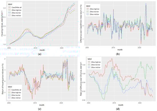
Figure 1.
Traditional and hedonic home price index comparisons. (a) Case–Shiller and Zillow valuation tiered housing price index; (b) Difference in returns relative to the national Case–Shiller (10 percent increment scale); (c) Monthly return indices (10 percent incremental scale); (d) Cumulative ratio Zillow tiers to the Case–Shiller national index.
While the end-level index values at the beginning of 2025 show similarities, the indices reveal significant dislocations during the Great Financial Crisis which was associated with potential housing bubbles. The housing dislocations related to the post-pandemic also show greater differences in the national indices. When visualizing the individual city data spread differences are often greater than reflected in national data; however, the patterns of all cities are not the same. There is a distinction between Sunbelt growth cities and Rustbelt contracting markets which show less HPI extremes.
The monthly return graph (Figure 1b) illustrates the greater volatility associated with the Case–Shiller index. Cyclical macroeconomic events have a greater impact on transactional prices than on broad hedonic housing valuation. Most monthly return differences fall within 5% per month; nevertheless, some periods during the GFC, housing recovery, and COVID show differences in return approaching 10% or more (Figure 1c). The cumulative difference between the high- and mid-tier markets reveals a significant behavioral distinction compared to the low-tier market (Figure 1d). Cheaper homes do not mean more stable prices, as entry-level buyers may exhibit higher levels of trade intensity than those purchasing high-end homes. Additionally, the value of lower-tier homes may diverge from higher tiers.
Local city markets show both common and city-specific variation. Figure 2a–d compare four cities for illustrative purposes. In the first case, Miami and Boston exhibit distinct price patterns, with Miami displaying strong price appreciation and notable divergences between HPIs. In the case of Boston, price appreciation is muted with smaller HPI return differentials. A comparison between Las Vegas and Los Angeles reveals that both cities experienced significant housing price appreciation following the market boom and bust that occurred during the Great Financial Crisis. The monthly return spread difference displays the variation in returns which are likely centered around macroeconomic events and potential local transaction congestion.
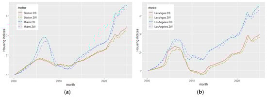
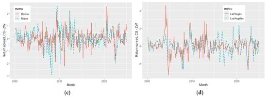
Figure 2.
Traditional and hedonic home price index comparisons for sample cities. (a) Traditional and hedonic (mid-tier) HPI for Miami and Boston; (b) Traditional and hedonic (mid-tier) HPI for Las Vegas and Los Angeles; (c) Traditional and hedonic (mid-tier) return spread for Miami and Boston; (d) Traditional and hedonic (mid-tier) return spread for Las Vegas and Los Angeles.
Localized real estate market factors create regional differences and impact spreads between transaction and hedonic indices. To display localized housing market differences, city housing betas are calculated based on the Case–Shiller National HPI, serving as the market portfolio due to its role as a standard index. There is a wide range of housing betas, with lower-tier homes showing higher levels. Cities such as Las Vegas, Phoenix, and Tampa SMSAs, which have seen significant population increases, show higher betas, (see Figure 3). These beta variations reinforce the observation that city-specific HPIs show greater variation than national data and may be more sensitive to economic variation and local market conditions.
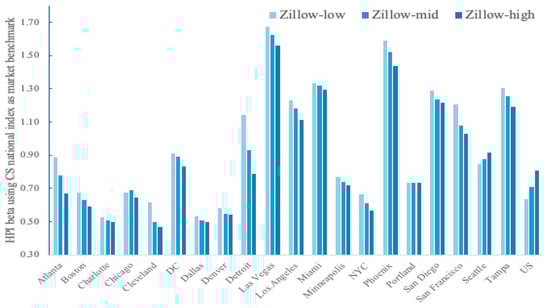
Figure 3.
Housing beta for city HPI with price tiers.
Both HPIs show strong positive autocorrelation with slow decay. Given the CS HPI construction as a moving average, this should be expected. The same effect is also present with the hedonic index, which uses transactional prices as a characteristic input. Housing shows strong momentum effects across all cities; however, using the augmented Dickey–Fuller test, all city HPIs are stationary at p-values below 0.01 when differenced. To show the link between the HPIs, we measured the cross-correlation between the CS city and Zillow city indices across tiers. Figure 4 displays the boxplots for different lead-lag times for the set of cities and tiers for the two HPIs, showing that Case–Shiller transactional index leads the movement in the Zillow hedonic index, peaking around the constructed CS lag structure.
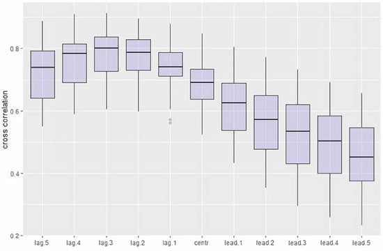
Figure 4.
Cross-correlation matrix. Note: There are 45 cases, fifteen cities with low, middle, and high-tier HPI for 2000–2024.
The stylized evidence of varying spread returns suggests that differences between the transactional and hedonic indices may be systematic due to the HPI construction. While the deviations between the two HPIs may not follow a universal pattern for every city, spreads between transactional and hedonic prices are associated with exhibited economic market behavior, especially at extremes. (A complete data set for all cities housing tiers is available upon request from the authors and will include charts of the difference between CS and ZVHI prices as well as return and ratio analysis. A full analysis of all city differences is beyond the scope of this paper which focuses on general return spread differences).
We next examine the data and test for systematic factors driving the index spreads, based on macroeconomic and housing-specific effects that may influence the willingness to transact versus the willingness to pay for localized housing valuation and buying behavior.
4. Exogenous Factors Describing Index Differences
The housing spreads comprise both time series and cross-sectional data for the city and value tiers and are impacted by both common and local variations. We model the ratio between the CS and ZH price index as
In the above model,
- Variables are common macro factors shared by metropolitan areas.
- Variable are local variables individual to each metro .
- The reflects the heterogeneity of each combination of metro and tier.
The difference in the log-price ratios is the log spreads, which is essentially the difference in log-price returns.
With the differencing, the is removed to simplify the analysis. Due to data limitations and time-series characteristics, we conduct two sets of analyses.
- The first study analyzes annual data spanning the period from 2000 to 2025 to examine the overall macro market conditions, including recession and growth, through the leading economic indicators index, mortgage rates, and local conditions such as unemployment rates and population changes, in a reduced form. We then add inventory data over a shorter period from 2016 to 2025.
- The second study analyzes monthly data from 2000 to 2025 and shorter periods with home inventory and time on the market. It includes overall macro conditions, such as recession and growth, as indicated by the leading economic indicators index and mortgage rates, as common factors. Additionally, it features local conditions, including unemployment rates, inventory levels, and median days on the market. The monthly data can utilize a shorter history and focus on these local factors to explain short-term variations in spreads.
We expect that panel data will exhibit heterogeneity, as already evident in the different city betas and variations in city standard deviations. While the return data are stationary, the cross-correlation suggests there is still potential for autocorrelation with residuals. The panel regression allows for the flexibility to include both common factors and local market conditions; however, there are still potential issues of heterogeneity, given that cities and value tiers will have different volatilities as described earlier. The Breusch-Pagan test of the OLS residuals from our model confirms heteroscedasticity.
To address these issues, we employ first-differenced flexible generalized least squares estimates (FGLS) for both our analyses using both longer and shorter-term data sets. The FGLS model is based on a two-step process of first estimating an OLS model with first differences and then using the residuals to estimate an error covariance matrix for use in a feasible GLS analysis which directly incorporates heteroscedasticity in the analysis. Diagnostic tests for multicollinearity suggest that our large data sample set and limited regressors do not exhibit characteristics that will impact econometric results. We test data across subperiods to measure regressor sensitivities.
4.1. Annual Panel Study for Transactional and Hedonic HPI Spreads
In our first study, we construct annual spread returns to mitigate autocorrelation effects using city and low, mid, and high value tiers to capture longer-term spread differences across 15 cities from 2001 to 2025. This allows us to calculate transactional minus hedonic returns over a more extended holding period and minimize the impact of any positive short-term autocorrelation. The panel regression reveals spread differences that are related to macroeconomic factors, such as interest rates and the business cycle. The results are presented in Table 3 for two periods, one covering the entire time series and the other a short period that allows for the inclusion of inventory data.
Table 3.
Transactional versus hedonic annual spreads, business cycle, and population changes Source: FRED data, CoreLogic, and Zillow websites.
Not all local markets will experience a downturn during a recession; however, some cities have faced significant downturns, as illustrated in our earlier figures. There is a negative association between the percentage of months in a recession during a given year and return spreads. If the local home market is in a national economic downturn, the CS index will underperform relative to the ZVHI index. As a macroeconomic growth proxy, we employ the index of leading economic indicators. There is a positive association with the HPI spread. Indications of stronger economic growth are tied to positive return spreads. The cost of capital, as measured by the 30-year mortgage rate, significantly impacts the willingness to transact and negatively drives return differences. The change in local unemployment also negatively affects return spreads, where unemployment has both a common macroeconomic component and a local city-specific component. Greater unemployment in an SMSA shows greater downward transaction pressure. City population demographic changes, which attempt to explain the Sunbelt/Rustbelt demographic shifts, show a negative, albeit insignificant, impact on return spreads.
The spread between transactional and hedonic HPIs decreases during recessions, periods of higher borrowing costs, and periods of negative expected growth (characterized by a common macro factor and higher local unemployment). Specifically, a weak (strong) macro or local economic environment results in the transactional HPI falling (rising) relative to hedonic price values. Differences between a willingness to transact and a willingness to pay create a dislocation between HPI methodologies.
The active listing count from Realtor.com is available from the FRED database starting in 2016. We add the local inventory change as a key feature for the local housing market effects. As a control, we test the existing macro features over the shorter time horizon. All signs are the same, with the local population change again being insignificant. This should not be surprising given the need for more extended periods to capture demographic changes. The recession indicator was dropped because the monthly recession change in 2020 was zero and there were no other recessions cine 2016. The local housing inventory change has a negative relationship, as local inventories rise, the spread difference will fall. Local inventory changes add to the multiple R-squared even with the shorter test period.
Increasing inventories are indicative of a buyer’s advantage market with increased choice and a greater willingness for sellers to reduce prices. Decreasing inventory reduces transactional choice and represents a seller’s advantage, which pushes transactional prices higher versus hedonic prices. Positive inventory changes are negatively associated with the HPI index return spread. High (increasing) inventory periods show transactional returns underperforming relative to hedonic returns, as sellers may need to lower prices to generate a transaction.
4.2. Monthly Panel Study for Transactional and Hedonic HPI Spreads
To examine these spread relationships more closely in localized housing markets over monthly periods, we compare the spread with local housing inventories, which serves as a proxy for whether a market is buyer- or seller-biased, using shorter datasets but increased samples. Although data is limited to the post-2017 period, Realtor.com also provides other local housing metrics, such as the median number of days on the market for each metro area. We add this feature to further reinforce the willingness to transact and impact the CS versus Zillow return spread relationship story. We again relate spreads to local unemployment changes and analyze common macro business conditions, as with the annual data. An increasing local unemployment rate is indicative of weak economic conditions and again shows a higher likelihood of forced selling and lower CS returns compared to Zillow.
Table 4 presents the panel data results again using the Flexible Generalized Least Squares (FGLS) model, which includes local home inventories and local median days on the market. Given the limitations of the local data, we compare across two different periods to test consistency with variable coefficients. The inventory data is available in 2016, so we test the general business regression for this shorter period and then conduct a second test that incorporates local inventory changes. We then add the change in median days on the housing market data since its availability in 2017.
Table 4.
Transactional versus hedonic annual spreads, business cycle, and inventory changes Source: FRED data, CoreLogic, Realtor.com, and Zillow websites.
The recession indicator, 30-year mortgage rates, and leading indicators all show similar signs and are consistent with the annual data. Macro features indicate that HPI spread differences are tied to changes in the common macro environment. Local unemployment changes are consistent with our base hypothesis of higher return spreads being associated with declining local unemployment rates.
Local housing inventory changes are relevant for the spread regressions, as well as the median days on the market for our short post-2018 period. The multiple R-squared values are lower than the annual tests but still show increases from the inclusion of local inventory changes, demonstrating the importance of macro and local housing conditions in explaining transactional versus hedonic return differences. On a further test of localized housing dynamics, city-specific OLS regressions of the monthly spread and inventory changes for three tiers and 15 cities over the 2016–2024 period show that inventory changes for a total of 43 of 45 regressions were significant and 38 of 43 showed a positive sign, with the inventory direction a key market indicator for explaining the difference between transactional and hedonic price HPI.
5. Discussion and Conclusions
Investors and policymakers have a keen interest in the housing market; however, comparative work on HPIs using different methodologies has not been conducted due to the constraints of data and markets for comparison. We address this issue by testing two alternative HPIs to explain when and why spread differences between HPI methodologies may occur, and conclude that the choice of index affects short-term housing market assessments. A policy focus that employs a transactional HPI will show more extremes and volatility than a hedonic index. The added volatility is associated with macro and localized factors that impact the willingness to transact. Hence, at market extremes, the transaction will peak and trough before a hedonic index and will suggest greater housing variation at both the national and city levels. While a transactional index reflects trading activity, its use may distort short-term wealth effects and market perceptions The choice of index should not be an afterthought, but rather a consideration for any analysis.
Although repeat-sales transactional and hedonic HPIs are highly correlated and closely match on an average month, there are structural and empirical differences that researchers should consider when choosing an HPI. These differences are primarily manifested in local city-specific price series. While the average monthly difference between a transactional and hedonic index will be less than 25 bps, there are months when the differences can be 200 to 400 basis points with monthly standard deviations exceeding one percent. These deviations are associated with economic business cycle extremes such as recessions or periods of high economic growth. The spread differences are also linked with local housing market conditions as expressed by home inventories and local unemployment. Hedonic prices may “catch-up” to transactional HPI, but analysts should realize that macro and local factors will create short-term price pressure effects in transactional indices.
A repeat sale transactional HPI will react more strongly to local and macroeconomic conditions, based on the willingness of buyers and sellers to transact versus a willingness to pay for housing characteristics. The Case–Shiller repeat-sale transactional HPI, leads the Zillow hedonic index and is more volatile. Extreme declines may be observed when using the Case–Shiller HPI, due to local downward pressure on transactions and issues with index inclusion of foreclosures. Downward sales pressure is driven by poorer economic conditions and/or poorer housing market dynamics resulting from distress, relative to an overall measure of housing value. Even with limited macroeconomic shocks (recessions), evidence suggests that the smoothed value-weighted Case–Shiller HPI will decrease (increase) more rapidly in a falling (rising) economic market versus a hedonic equal-weighted median characteristic (ZHVI) HPI. These price deviations accentuate short-term beliefs in housing extremes or bubbles.
The ZVHI index series provides more broad-based information with greater granularity for any micro-spatial analysis. Employing hedonic information, such as ZHVI, in localized analysis may benefit policymakers and housing researchers through providing a more comprehensive description of the housing market that is not overly weighted toward short-term transaction behavior; however, creating a hedonic price index introduces greater complexity, especially one that utilizes machine learning (neural network) procedures. While utilizing the foundation frameworks found in other publicly available (government-generated) hedonic HPIs, Zillow, with its proprietary machine learning model, is less transparent than a repeat-sales index. Limitations in forming any price index based on measuring dynamic characteristics must be balanced against limitations from constrained repeat sales transactional data that control for quality. Nonetheless, our analysis shows that, on average, the monthly differences across these two methodologies are similar, albeit with wide ranges. Both may closely track what may be called the actual home value of a given geography. Hence, it is difficult to argue that one HPI approach is superior to another based on return deviations.
Our novel results help explain the factors that lead to differences in return spreads across different HPI methodologies; nevertheless, there are broader issues than measured differences in the construction of housing price indices. One, how much reliance should users place on different HPI methodologies? Two, how much transparency should be associated with an index that may be used in the role of a public good? Three, what should be the role of private firms in generating public information, and how much effort should governments place in HPI construction? Public versus private generation of data, like issues of transparency, are not easy to answer, yet must be considered when using information for research and policy decisions.
The measured spreads between US transactional and hedonic indices generate a greater appreciation of differences in global housing indices, as the construction of OECD housing price indices varies across countries. For example, the strong use of a repeat sales transactional HPI versus hedonic HPI in Europe may suggest that US housing markets are more volatile, when in fact the driver for differences may be based on methodology. There is precedent for a multi-pronged HPI approach given mixed data from the OECD, where countries differ in their methodologies for housing price indices.
Nevertheless, the integration of a proprietary hedonic price index into research and policy applications should be predicated on increased transparency in index construction. Currently, the Case–Shiller transactional index has methodological transparency, and the OECD housing indices are subject to established guidelines within a handbook. Although descriptions accompany them, the hedonic Zillow indices are proprietary and do not provide full transparency, making them difficult to replicate, which limits their role as a benchmark, even if they are readily available. Further research is needed to focus on the impact of transaction return data versus data based on characteristics that may represent the fair value within a localized housing market, to improve our understanding of housing price dynamics. Our research suggests that tracking both a volatile transaction index and a characteristic-based hedonic index may yield a more accurate estimate of regional housing values.
Author Contributions
Conceptualization, M.R.; methodology, M.R. and W.F.; software, W.F.; validation, M.R. and W.F.; formal analysis, M.R. and W.F.; investigation, M.R. and W.F.; resources, W.F.; data curation, W.F.; writing—original draft preparation, M.R.; writing—review and editing, M.R. and W.F.; visualization, W.F.; supervision, M.R.; project administration, M.R. All authors have read and agreed to the published version of the manuscript.
Funding
This research received no external funding.
Institutional Review Board Statement
Not applicable.
Informed Consent Statement
Not applicable.
Data Availability Statement
All data are available from the FRED database, CoreLogic, Zillow website, or Realtor.com.
Acknowledgments
We acknowledge support through comments from the reviewers.
Conflicts of Interest
The authors declare no conflicts of interest.
Appendix A
Table A1.
Alternative Housing indices.
Table A1.
Alternative Housing indices.
| Characteristics | FHFA | Freddie Mac FMHPI | National Association of Realtors (NAR) | Redfin | Census Bureau | Realtor.com |
|---|---|---|---|---|---|---|
| Objective | Sample of GSE-backed loans | Freddie Mac and Fannie Mae portfolio | Broad index focused on real estate professional | Repeat Sales transactional data | New construction index | Listing price analysis with market trend calculation |
| Methodology | Repeat sales for conforming loans | Repeat sales from within portfolio | Median sale price from actual sale transactions | MLS sales and public record data | New construction using median price | Listing and sales data |
| Source Data | Fannie and Freddie Mac | Fannie and Freddie Mac | Actual closed sales using MLS data | Redfin’s database from MLS data | New home sales, building permits and construction survey data | Listing and sales data |
| Scope | National, census division and states | National | National and four regions (West, Midwest, South, and Northeast | National, state, metro, and local market indices | National, regional based on census tracts and selected metro areas | National, state, metro, county, and zip code data |
| Inclusion | Single-family homes; no cash sales or jumbos | Single-family homes | Median of home, condo, and co-op sales; no adjustment for size and quality | Repeat sales methodology | New single-family homes, housing units and construction activity | Active listings, sold properties and price trends from MLS data |
| Frequency | Monthly national; quarterly for states | Monthly | Monthly | Monthly | Monthly and annual data | Monthly and weekly data |
| Periodicity | From 1975 | From 1975 | From 1968 | From 2012 | From 1963 | From 2008 |
References
- Duca, J.; Muellbauer, J.; Murphy, A. What Drives House Price Cycles? International Experiences and Policy Issues. J. Econ. Lit. 2021, 59, 773–864. [Google Scholar] [CrossRef]
- Glaeser, E.; Gyourko, J. The Economic Implications of Housing Supply. J. Econ. Perspect. 2018, 32, 3–30. [Google Scholar] [CrossRef]
- Bhar, R.; Malliaris, A.; Malliaris, M.; Rzepczynski, M. Five Themes of U.S. Home Prices Cycles: A Dynamic Modelling approach. Ann. Oper. Res. 2024, 4, 1–21. [Google Scholar] [CrossRef]
- Gallin, J.; Molloy, R.; Nielsen, E.; Smith, P.; Sommer, K. Measuring Aggregate Housing Wealth: New Insights from Machine Learning. J. Hous. Econ. 2021, 51, 101734. [Google Scholar] [CrossRef]
- Dorsey, R.E.; Hu, H.; Mayer, W.J.; Wang, H. Hedonic Versus Repeat-Sales Housing Price Indexes: A Comparison of Methodologies. Real Estate Econ. 2010, 38, 239–266. [Google Scholar]
- Case, B.; Pollakowski, H.; Wachter, S. Frequency of transaction and house price modeling. J. Real Estate Financ. Econ. 1997, 14, 173–187. [Google Scholar] [CrossRef]
- Gatzlaff, D.; Haurin, D. Sample selection bias and repeat-sales index estimates. J. Real Estate Financ. Econ. 1997, 14, 33–50. [Google Scholar] [CrossRef]
- Doerner, W.; Leventis, A. Distressed Sales and the FHFA House Price Index. J. Hous. Res. 2015, 24, 127–146. [Google Scholar] [CrossRef]
- Glaeser, E.; Gyourko, J. The Impact of Zoning on Housing Affordability. Econ. Policy Rev. 2003, 9, 21–39. [Google Scholar]
- Silver, M. How to better measure hedonic residential property price indexes. In Proceedings of the 2016 Conference of the Society of Economic Measurement, Thessaloniki, Greece, 6–8 July 2016. IMF Working Paper, WP/16/213. [Google Scholar]
- Calhoun, C. OFHEO House Price Indexes: HPI Technical Description; Office of Federal Housing Enterprise Oversight: Washington, DC, USA, 1996. [Google Scholar]
- Hill, R. Hedonic Indices for Housing; OECD Statistics Working Papers: Paris, France, 2011; Volume 1. [Google Scholar]
- Handbook of Residential Property Prices Indices (RPPIs), a Eurostat Methodologies and Working Paper. 2013. Available online: https://ec.europa.eu/eurostat/web/products-manuals-and-guidelines/-/ks-ra-12-022 (accessed on 1 July 2025).
- Case, K.; Shiller, R.; Weiss, A. Index-Based Futures and Options Markets in Real Estate. J. Portf. Manag. 1993, 19, 83–92. [Google Scholar] [CrossRef]
- Shiller, R. Understanding Recent Trends in House Prices and Home Ownership; NBER Working Paper; National Bureau of Economic Research: Cambridge, MA, USA, 2007; p. 13553. [Google Scholar]
- Humphries, S.; Fleming, M. Lunchtime Data Talk IV—Home Price Indices: Appreciating the Differences White Paper. 2013. Available online: https://wp.zillowstatic.com/3/D_LDTAppreciatingtheDifferences091313-55384b.pdf (accessed on 1 September 2025).
- CoreLogic. U.S. Home Price Insights: Methodology and Comparison to S&P CoreLogic Case-Shiller Index; CoreLogic White Paper: Irvine, CA, USA, 2020. [Google Scholar]
- S&P. Dow Jones Indices S&P CoreLogic Case-Shiller Home Price Indices Methodology; S&P: Manhattan, NY, USA, 2024. [Google Scholar]
- Zillow Research. Case-Shiller Revisions Bring It More in Line with the Zillow Home Value Index; Zillow Research Blog; Zillow Research: Seattle, WA, USA, 2014; Available online: https://www.zillow.com/research/case-shiller-revision-june-2014-7831/ (accessed on 1 September 2025).
- Nagaraja, C.; Brown, L.; Zhao, L. An Autoregressive Approach to House Price Modeling. Ann. Appl. Stat. 2011, 5, 124–149. [Google Scholar] [CrossRef]
- Glynn, C. Learning low-dimensional structure in house price indices. ALPPL Stoch. Models Bus. Ind. 2022, 38, 151–168. [Google Scholar] [CrossRef]


Disclaimer/Publisher’s Note: The statements, opinions and data contained in all publications are solely those of the individual author(s) and contributor(s) and not of MDPI and/or the editor(s). MDPI and/or the editor(s) disclaim responsibility for any injury to people or property resulting from any ideas, methods, instructions or products referred to in the content. |
© 2025 by the authors. Licensee MDPI, Basel, Switzerland. This article is an open access article distributed under the terms and conditions of the Creative Commons Attribution (CC BY) license (https://creativecommons.org/licenses/by/4.0/).