Abstract
Urban transformations require balancing private real estate interests with the provision of public spaces that enhance sustainability and ecosystem services. This study proposes a probabilistic model to assess the feasibility of transforming buildable areas while ensuring equitable benefits for both private developers and public administrations, with a focus on three areas to be regenerated within the Municipality of Lucca as case studies. Applying the Monte Carlo (MC) method, two probabilistic models—one with a Uniform distribution and the other with a Normal distribution—estimate the expected Transformation Value (TV) and its associated uncertainty. Results highlight the effectiveness of MC-based assessments in managing financial uncertainty, aiding developers in risk evaluation, and supporting policymakers in designing balanced urban planning indices. It was observed that the Uniform model is better suited to situations in which the initial values of the model’s main variables—such as construction costs, post-transformation market value, or transformation duration—are not fully known, whereas the Normal model provides more accurate estimates when the investment scenario is better understood. The results demonstrate that this approach provides, on the one hand, a robust tool for investment risk analysis to private investors and, on the other hand, a way for public institutions to verify whether urban planning indices enable private promoters to contribute effectively to the development of sustainable cities.
1. Introduction
The concepts of urban rent and the value of buildable land have been extensively analyzed in academic literature over the years [1,2]. In contemporary urban planning, there is an increasing emphasis on sustainable land use and the need to strike a balance between economic development and environmental preservation [3,4,5,6]. The dynamic nature of the real estate market further complicates this balance, making it crucial to evaluate the economic feasibility of transforming buildable areas while ensuring that urban development aligns with public interest [7,8,9]. In this context, the calibration of urban planning indices plays a fundamental role in achieving equilibrium between private investment objectives and broader societal benefits. For instance, a critical index is the so-called building index, defined as the ratio between the buildable volume of a land parcel and its total surface area [10]. Urban planning indices are essential for private landowners and [11,12,13] developers, as they determine the extent of permissible construction and, consequently, the potential return on investment [14].
This issue gains even greater significance when considering urban regeneration projects targeting degraded, unused, or undeveloped areas within already urbanized perimeters [7,8,15,16,17,18,19]. In such cases, the added value of transformation projects is increasingly associated with environmental and social improvements rather than just the physical modification of spaces. This shift in focus reflects a broader recognition that urban transformations should not merely address real estate market demands but also contribute to the quality of life, ecosystem services, and public welfare.
Historically, the governance of buildable land transformation has evolved toward more collaborative approaches. In recent decades, urban planning has increasingly embraced models based on Public–Private Partnerships (PPPs), which formalize cooperation between local governments and private developers to jointly manage urban regeneration initiatives [20,21,22]. This approach allows for greater flexibility in designing transformation strategies, promoting shared responsibilities in financing, implementation, and benefit distribution. As highlighted in the literature, PPPs are often seen as a pragmatic tool to align private investment capacity with public objectives, especially in contexts requiring substantial infrastructure development, environmental remediation, or the provision of social services.
However, the adoption of PPP frameworks has also raised critical concerns regarding transparency, accountability, and the equitable allocation of value generated through urban transformation processes. In some cases, decisions made without adequate consideration of social and economic repercussions led to disproportionate advantages for private developers, while public benefits remained insufficiently addressed [23,24,25].
One of the primary mechanisms intended to balance private profits with public interest has been the application of urbanization charges, which require developers to contribute to the infrastructure and services necessary to accommodate new developments [21,22]. However, this system has faced criticism for potentially discouraging investment in real estate and exacerbating existing weaknesses in the construction sector [26]. These debates highlight the ongoing challenge of defining urban planning tools that ensure both financial sustainability for private investors and the adequate provision of public amenities [27].
A key concept in evaluating the economic feasibility of urban transformations is the TV, which represents the difference between the Market Value (MV) of a developed property and the total costs associated with its transformation [28]. In Italy, the calculation of TV follows methodologies outlined in the MOSI Manual [29]. However, traditional valuation methods often struggle to accommodate the uncertainties inherent in real estate investments, particularly those related to fluctuations in construction costs, market demand, and regulatory changes. To address these challenges, probabilistic modeling techniques—such as the MC—have gained prominence as tools for quantifying and managing uncertainty in financial projections [15,30,31,32,33,34,35,36].
Indeed, the MC is a numerical simulation technique which enables the resolution of complex problems by incorporating probabilistic distributions rather than relying on fixed deterministic input values. Over time, advancements in algorithmic development and statistical sampling techniques have significantly enhanced the precision and applicability of these methods, making it a valuable tool in real estate evaluation and urban planning [15,34,37].
Accordingly, this study employs the MC method to evaluate the feasibility of transforming buildable areas while ensuring a balanced distribution of benefits between private developers and public administrations. The research focuses on three case studies selected within the Land Use Plan (LUP) of the Municipality of Lucca (Piano Operativo della Città di Lucca), Italy, which outlines specific urban planning regulations and transformation guidelines for vacant areas within the urbanized territory of the city. Through probabilistic modeling, this study assesses the likelihood of achieving a favorable TV under varying economic and technical conditions.
2. Materials and Methods
The methodological framework of this study is structured around a probabilistic modeling approach, utilizing the MC method to evaluate the feasibility of urban transformation projects. The analysis involves defining key parameters, incorporating uncertainty in economic and technical variables, and conducting simulations to assess outcomes in different scenarios. This section details the conceptual structure of the model, the MC simulation process, and the data selection criteria used in the study.
2.1. Conceptual Model and Approach
As stated previously, the proposed model aims to assess the TV of buildable areas, considering both economic feasibility and public–private balance in urban transformations. The LUP provides specific regulatory guidelines for the transformation of selected areas, which define:
- the urban planning parameters applicable to private areas;
- the land surfaces to be transferred to public use, in accordance with specified urban planning standards and indices;
- the financial private contributions required for primary and secondary urbanization of the areas.
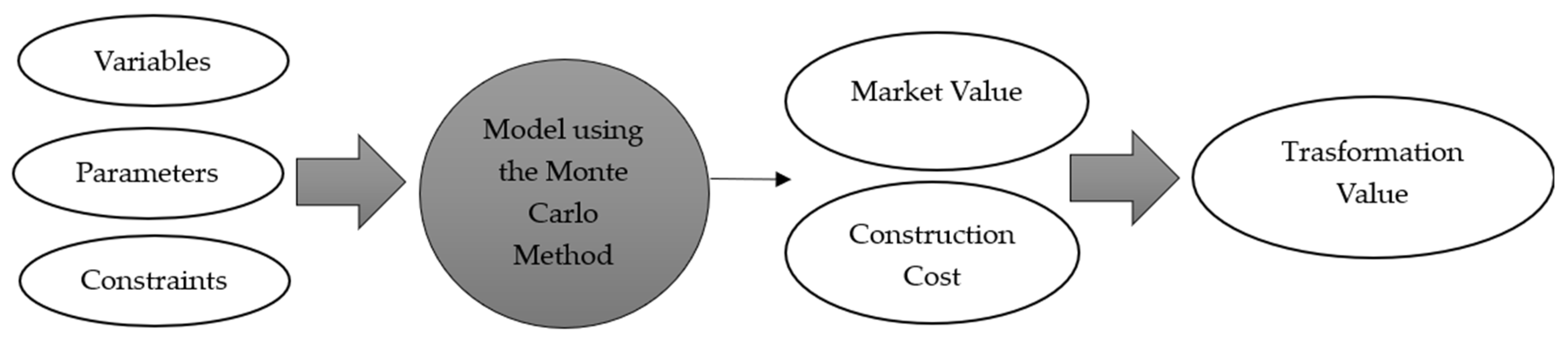
Figure 1 illustrates the essential steps that form the basis of the proposed framework. The first step involves defining the so-called simulation parameters, input variables, and system constraints of the MC-based models. Simulation parameters are fixed values defined by the user and remain constant throughout the MC simulations, while input variables represent numerical values that can vary within a specified range. Constraints refer to specific limits that the models must respect, as determined by local regulations and the planning standards outlined in the LUP sheets.

Figure 1.
Workflow of the proposed model.
Once the variables, parameters, and constraints are defined, the Monte Carlo model allows the calculation of the Market Value (MV), the Construction Costs (CC), and consequently the Transformation Value (TV). The core research question is whether the transformation of these areas is economically viable for both private developers and public administrations, taking into account their respective interests in the transformation process.
2.2. Model Implementation and Calculation Process
The first step to perform MC involves defining the parameters, variables, and constraints that govern urban transformations. Parameters include fixed values dictated by zoning regulations, urbanization charges, and municipal guidelines. Variables represent economic and technical factors that fluctuate based on market conditions, such as construction costs, real estate prices, and financial charges. Constraints ensure compliance with urban planning requirements, such as minimum public land allocations, debt ratio regulations, and public parking standards.
Once these inputs are defined, the model computes the TV, representing the difference between the MV of developed properties and the total costs (C) incurred in the transformation process. It is worth noting that, in this study, the MV is defined following EU Regulation n. 575/2013 [38], which states: “The estimated amount for which the property would be sold at the valuation date in a transaction carried out between a willing seller and a willing buyer under normal market conditions, following adequate marketing, and where both parties have acted knowledgeably, prudently, and without compulsion”.
The aforementioned definition aligns with the valuation approach applied in this study, as it ensures that MVs are determined based on transparent, standardized criteria. To operationalize this principle within the MC simulation, MV estimations rely on OMI data from the Italian Agenzia delle Entrate (https://www1.agenziaentrate.gov.it/servizi/Consultazione/ricerca.htm?level=0, accessed on 15 March 2025), which provides empirical benchmarks for real estate pricing. The use of probabilistic modeling further refines this estimate by incorporating fluctuations in market conditions, property characteristics, and economic variability. The OMI value refers to real estate units in normal (i.e., ordinary) maintenance conditions. However, the transformation areas under analysis are intended for new developments, which generally achieve higher market values. Consequently, a 30% increase has been applied to the OMI benchmarks to reflect the typical price difference between existing stock and new constructions, as observed in local real estate markets. It is worth noting that, in practical applications, this uplift should be refined through market surveys, relying on comparable sales of newly built properties in the relevant urban context. The adjusted OMI value is then bounded within a ±10% range for MC simulations (details in Section 2.4). The MV per square meter is then multiplied by the maximum buildable area (BA) to obtain the estimated total MV, as expressed in Equation (1):
where BA represents the maximum buildable area specified within the regulatory sheets.
As said, the model also integrates C, which include technical costs, urbanization charges, professional fees, general expenses, marketing costs, financial charges, and developer profit margins. Equation (2) outlines the cost structure:
where:
- represents the technical transformation cost, which includes the cost of constructing covered areas, private green spaces, and private parking;
- and refer to the urbanization charges and construction cost contributions, both defined by the Municipality of Lucca based on the area and type of intervention;
- represents professional fees, which are the costs of professional services, expressed as a percentage of the technical transformation cost;
- represents general expenses, calculated as a percentage of the sum of the technical transformation cost and urbanization charges;
- represents marketing and sales expenses, calculated as a percentage of the ;
- represents financial charges, a variable that fluctuates over time and is calculated based on the average annual interest rate and the duration of the transformation;
- is the profit of the promoter, which is the return derived from investing capital in the real estate project. It depends on the average annual interest rate and the duration of the operation.
Mean, minimum, and maximum values of the aforementioned components of C, to be used in MC simulations, have been detailed in Section 2.4. Once MV and C have been computed, the calculation of TV follows Equation (3):
where represents the total duration of the transformation in years, is the discount ratio that accounts for the time value of money, and are the indirect costs and financial charges related to land capital, expressed as a percentage of the TV, computed as follows in Equation (4):
where IC represents the indirect acquisition costs related to land capital, in which computation is related to the TV. These costs are estimated assuming that the property transfer is subject to a 9% registration tax (according to the Italian Revenue Agency), plus a 2% mortgage tax and a 1% cadastral tax, for a total of 11%. Additionally, notary fees and other ancillary expenses are estimated at 4% of the value, bringing the total acquisition costs to 15% of the TV.
The discounting process is essential to ensure that property valuations reflect present market conditions, rather than speculative future values. The discount rate is derived from risk-free government bond rates with a duration comparable to real estate projects, which are equal to 3.861% (derived from Bank of Italy, https://www.bancaditalia.it/compiti/operazioni-mef/rendistato-rendiob/documenti/rendistato-2023.pdf, accessed on 15 March 2025).
It is also worth noting that, in the analyzed use cases, the expected duration of the projects are set at 30 months. Nonetheless, to incorporate potential delays, the MC simulations extend this timeframe up to 36 months, representing a 20% increase over the initially planned duration. This accounts for potential setbacks in authorization procedures, construction delays, and market fluctuations that may affect the transformation timeline.
The final step in the simulation process is the analysis of the probability distribution of resulting TVs. Two versions of the model are used: the Uniform (or Random) model, where input values fluctuate randomly within a defined range, and the Normal (or Gaussian) model, which assigns higher probabilities to values closer to the mean according to a Normal probability density function. The output includes the average TVs, the unit TVs, and the probability of achieving a TV within ±10% of the mean value. By comparing the two models, the study provides insights into how investment risk varies based on the assumed probability distribution of input variables.
2.3. Data Selection and Case Study Parameters
The study is based on three use cases identified within the LUP of the Municipality of Lucca, each representing different urban transformation scenarios (https://maps3.ldpgis.it/lucca/?q=po, accessed on 15 March 2025). These cases were selected based on their classification as degraded, unused, or undeveloped areas, their inclusion in the zoning regulation sheets, and the availability of documented urban planning constraints and financial parameters. The selection of these use cases also considers economic feasibility, ensuring that transformations align with real estate market conditions while remaining compliant with regulatory constraints. Therefore, the primary goal is to analyze whether these transformations can achieve an equitable balance between public and private interests while remaining financially sustainable.
Table 1 presents the key parameters defining the three use cases, including size of the area, buildable land, public land allocation, urbanization charges (primary and secondary), and contribution to the construction costs.

Table 1.
Model parameters.
The public land allocation component is particularly significant, as it represents the portion of the buildable area that must be transferred for public use, ensuring compliance with urban planning standards. From Table 1, it is possible to observe that, in all three case studies, a significant percentage of land is allocated to public spaces, reflecting the efforts of the Municipality of Lucca to prioritize sustainability, green infrastructures, and social well-being.
2.4. Selection of Variables and Constraints
The MC-based models incorporate a range of stochastic variables whose values fluctuate according to a specified distribution within a defined range, reflecting market volatility and financial uncertainty. These variables include construction costs, real estate market prices, professional fees, financial charges, and transformation duration. For each variable, the minimum, maximum, mean, and standard deviation values have been defined by considering data from municipal regulations, construction industry reports, and real estate market trends. They are reported in Table 2.
Table 2.
Input variables of MC models.
The variables have been selected to reflect the economic uncertainties affecting urban transformations. For example, residential construction costs are influenced by material price fluctuations, labor costs, and technological advancements in building efficiency. Similarly, OMI values are subject to real estate demand trends, macroeconomic conditions, and local property valuation policies.
Regarding the construction costs, the price indications from the DEI Manual have been used [39]. As for the percentages on expenses and fees, the MOSI Manual was considered [29]. The OMI value and the total project duration have been previously discussed.
As an instance, Figure 2 shows the values of residential construction costs by employing different distributions (Uniform and Normal).
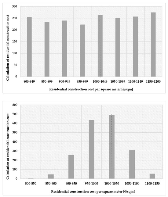
Figure 2.
Difference in the distribution of residential construction cost per square meter between the two models. Above: Random model; below: Normal model.
In addition to these variables, the model is constrained by specific urban planning regulations, ensuring that transformations comply with legal and financial benchmarks. Table 3 outlines the constraints considered by the MC-based models, covering public area allocation, debt ratio, and public parking area requirements.
Table 3.
Model constraints.
Specifically, the number of inhabitants is calculated by dividing the total built volume by 100. The minimum public surface area follows the Ministerial Decree of 2 April 1968, n. 1444 [40], which mandates at least 18 m2 per inhabitant, divided into spaces for education (4.50 m2), community services (2.0 m2), parking lots (2.50 m2), and green areas (9 m2). The debt ratio, regulated by the Basel Committee on Banking Supervision, ensures financial sustainability by keeping borrowing levels between 20% and 60% [41]. The public parking allocation, governed by Law 24 March 1989, n. 122 [42], mandates that 1 m2 of parking area must be provided for every 10 m3 of constructed volume. These constraints are incorporated into the MC simulations, ensuring that generated TVs comply with these regulations.
It is worth noting that, while the three selected case studies are located within the Municipality of Lucca, the applicability of the model is not limited to this specific context. The core structure of the model relies on parameters and constraints that are common across many Italian municipalities. As such, the methodology is expected to maintain a high degree of generalizability in similar regulatory environments. Adaptation to other geographic contexts would require recalibration of input variables based on local planning standards and real estate benchmarks, which is feasible using the same probabilistic framework presented herein.
3. Results
The MC simulations applied to the three selected case studies provide insights into the economic feasibility of urban transformations, the probability distributions of the TV, and the impact of different modeling assumptions on risk assessment. The results are presented in three key sections: (1) TV Computation, Distributions, and Descriptive Statistics, (2) Comparison of the Uniform and Normal models, and (3) Stability tests.
3.1. Transformation Value Computation, Distributions, and Descriptive Statistics
The primary outcome of the MC simulations is the estimated TV for each case study. Table 4 presents the TV under both Uniform and Normal probability distribution models. Table 4 reports the average TV, the unit TV (in terms of €/m2), and the probability of obtaining a TV within 10% range of the mean value.
Table 4.
TV and unit TV estimations in Uniform and Normal models.
Table 4 highlights both the similarities and differences between the two probabilistic models. The average TV and the unit TV remain largely consistent, with deviations below 2% across all three cases). Nonetheless, the Normal model consistently shows a higher probability (around 43%) of achieving a TV within ±10% of the mean, compared to the Uniform model (~30%).
This outcome was expected, as the probability density function of the Normal distribution tends to concentrate values more closely around the mean. By contrast, the Uniform model accounts for greater uncertainty in the estimation of input variables. In fact, during each MC simulation, input values are drawn randomly and uniformly from a defined range, without any preference for central values.
Therefore, in investment scenarios characterized by a high risk of misestimating input variables—such as those highlighted in Table 2—the use of a Uniform distribution enables the model to incorporate this uncertainty explicitly. At the same time, it still provides Transformation Value estimates that are consistent with those produced by the Normal distribution, indicating no significant bias. Furthermore, the Uniform distribution remains a valid option when precise knowledge of input values is unavailable, as long as a plausible minimum and maximum are defined.
In this regard, the Uniform distribution proves to be a viable and robust alternative to the more traditional Normal distribution when modeling uncertainty in urban transformation assessments.
3.2. Comparison of the Uniform and Normal Models
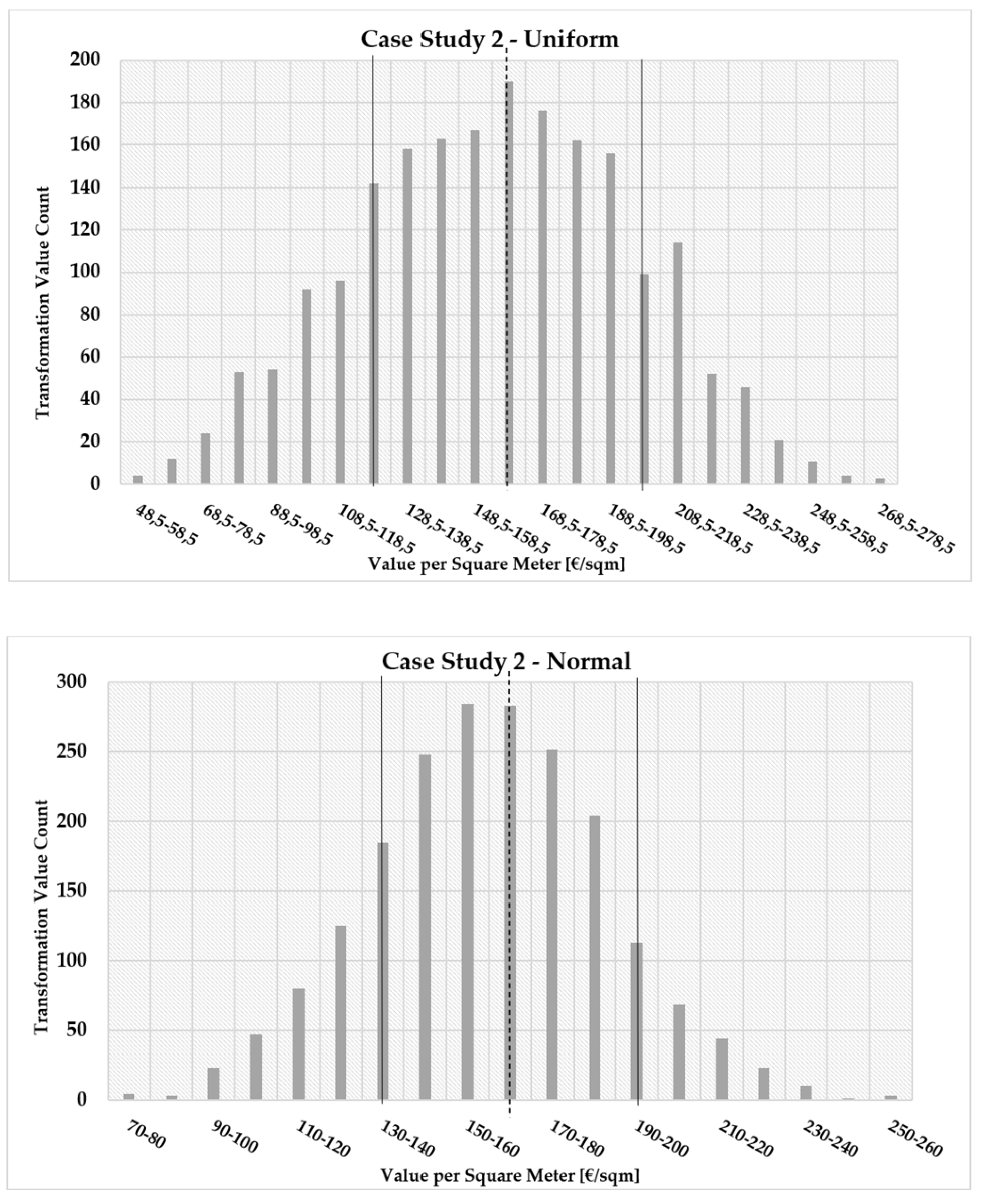
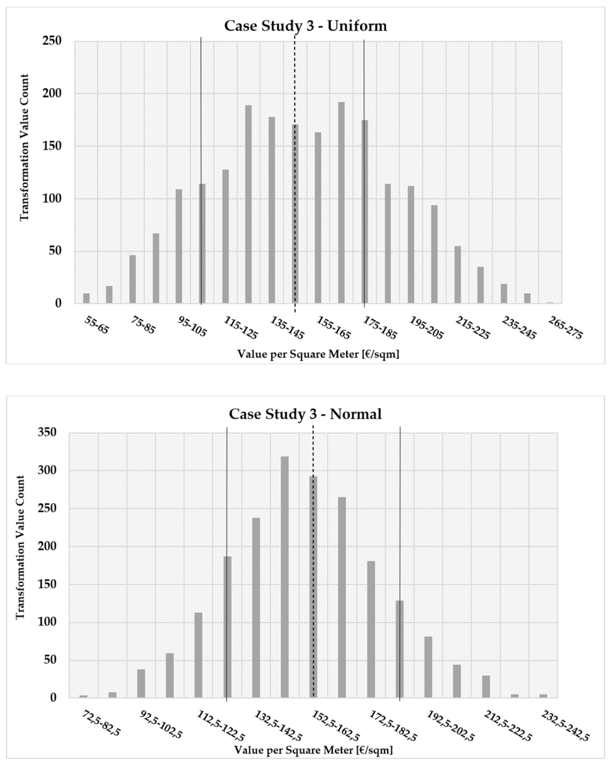
To further understand the impact of input variable distributions on resulting TVs, Figure 3, Figure 4 and Figure 5 present the probability distribution of unit TV for each case study, comparing the outcomes obtained using Uniform and Normal input distributions.
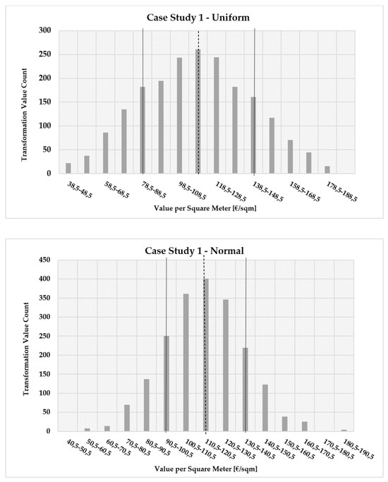
Figure 3.
Distribution of per m2 in Uniform (top) and Normal (bottom) models—Case Study 1.
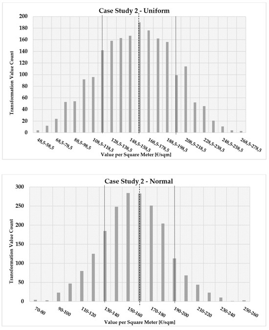
Figure 4.
Distribution of per m2 in Uniform (top) and Normal (bottom) models—Case Study 2.
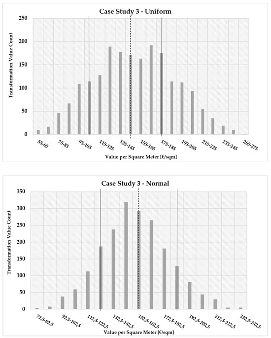
Figure 5.
Distribution of per m2 in Uniform (top) and Normal (bottom) models—Case Study 3.
As shown, the Uniform model generates a broader and more dispersed distribution compared to the Normal model, indicating a higher degree of uncertainty in the estimation of the TV. In contrast, the Normal model produces a tighter concentration of values around the mean, reflecting greater confidence in the scenario assumptions.
A closer look at the distributions reveals that the frequency with which the mean TV is achieved differs significantly between the two models. For instance, in Case Study 1, the mean TV (indicated by the vertical dashed line) is observed in approximately 400 Monte Carlo simulations under the Normal model, while it appears in only about 250 simulations under the Uniform model (i.e., representing a substantial 60% decrease). Similar patterns are observed in the other case studies, confirming the increased dispersion associated with the Uniform distribution.
Additionally, Figure 3, Figure 4 and Figure 5 include two solid vertical lines indicating the ±10% range around the mean value. In Case Study 1, for example, approximately 1480 simulations fall within this range when using the Uniform distribution, compared to about 1580 simulations under the Normal distribution. This further supports the observation that the Normal model yields results more tightly clustered around the mean, making it more suitable for scenarios in which greater certainty regarding input variables is available.
To further analyze the two models, Table 5 presents the descriptive statistics of the unit TVs derived from the Uniform and Normal distributions across the three case studies. Specifically, Table 5 includes the following:
- Mean and standard deviation, indicating central tendency and variability, respectively. Standard deviation is particularly relevant for assessing the degree of uncertainty associated with the input parameters; a higher standard deviation suggests greater potential risk or variability in project outcomes;
- Minimum and maximum values, which define the range of possible outcomes. These values allow for a preliminary assessment of best- and worst-case scenarios, offering valuable input for risk analysis and decision-making;
- Skewness and kurtosis, which describe the shape of the distribution. Skewness measures asymmetry: positive values indicate a right-skewed distribution, while negative values indicate left-skewness. Kurtosis evaluates the “peakedness” of the distribution: higher values imply a sharper peak, while negative values indicate a flatter distribution.
Table 5.
Descriptive statistics of the Uniform and Normal models among case studies.
Table 5.
Descriptive statistics of the Uniform and Normal models among case studies.
| Case 1 Uniform | Case 1 Normal | Case 2 Uniform | Case 2 Normal | Case 3 Uniform | Case 3 Normal | |
|---|---|---|---|---|---|---|
| Mean (€/m2) | 111.81 | 113.96 | 158.75 | 159.46 | 153.05 | 153.97 |
| St. Dev. (€/m2) | 29.74 | 20.14 | 40.72 | 27.84 | 39.27 | 26.6 |
| Kurtosis | −0.51 | 0.12 | −0.47 | 0.059 | −0.58 | −0.071 |
| Skewness | 0.051 | 0.047 | −0.038 | 0.043 | 0.038 | 0.11 |
| Minimum (€/m2) | 38.39 | 40.39 | 48.38 | 69.76 | 54.92 | 72.03 |
| Maximum (€/m2) | 193.84 | 185.48 | 274.53 | 258.87 | 270.43 | 238.11 |
From Table 5, it is evident that the mean unit TV values are nearly identical between the two models. However, the other descriptive statistics offer additional insights that help characterize the differences:
- Case 1—Uniform: The mean value is 111.81 €/m2, with a standard deviation of 29.75 €/m2. The minimum value is 38.39 €/m2, and the maximum value is 193.84 €/m2, denoting a favorable urban transformation. However, the data exhibit a slight positive skewness (skewness = 0.051) and a relatively flat distribution (kurtosis = −0.51). The positive skewness is not ideal, as it suggests that the number of iterations with values greater than the mean unit TV is smaller compared to those with results lower than the mean value per square meter. Negative kurtosis values are also not optimal because they indicate a flatness in the distribution;
- Case 1—Normal: The mean value is 113.96 €/m2, with a standard deviation of 20.14 €/m2. The minimum value is 40.39 €/m2, and the maximum value is 185.47 €/m2, which is still favorable. In this case, there is again a slight positive skewness (skewness = 0.047) and a relatively elongated distribution (kurtosis = 0.12). While the positive skewness is still suboptimal, the positive kurtosis is better since it reduces dispersion of values around the mean value;
- Case 2—Uniform: The mean value is 158.75 €/m2, with a standard deviation of 40.72 €/m2. The minimum value is 48.38 €/m2, and the maximum value is 274.53 €/m2. The data show a slight negative skewness (skewness = −0.04) and a relatively flat distribution (kurtosis = −0.467). The negative skewness is favorable as it indicates that the number of iterations with values greater than the mean unit TV is greater than those with values less than the mean. However, the negative kurtosis is suboptimal;
- Case 2—Normal: The mean value is 159.46 €/m2, with a standard deviation of 27.84 €/m2. The minimum value is 69.76 €/m2, and the maximum value is 258.87 €/m2. The data exhibit a slight positive skewness (skewness = 0.043) and a relatively elongated distribution (kurtosis = 0.06). As in the previous cases, the positive skewness is not ideal, while the positive kurtosis is favorable;
- Case 3—Uniform: The mean value is 153.05 €/m2, with a standard deviation of 39.27 €/m2. The minimum value is 54.92 €/m2, and the maximum value is 270.43 €/m2. The data show slight positive skewness (skewness = 0.04) and a relatively flat distribution (kurtosis = −0.58). Both positive skewness and negative kurtosis are suboptimal;
- Case 3—Normal: The mean value is 153.97 €/m2, with a standard deviation of 26.60 €/m2. The minimum value is 72.03 €/m2, and the maximum value is 238.11 €/m2. The data again exhibit slight positive skewness (skewness = 0.11) and a relatively flat distribution (kurtosis = −0.071). Both positive skewness and negative kurtosis are suboptimal.
In general, the lower standard deviation observed in all three cases using the Normal model suggests reduced variability and confirms its greater stability when estimating the TV. As for kurtosis, all three use cases under the Uniform model show negative values, indicating that the resulting distributions are flatter than the Normal distribution. Under the Normal model, negative kurtosis is observed only in Case Study 3, while Cases 1 and 2 show slightly positive values, suggesting a more desirable peaked shape. Regarding skewness, it is positive in five out of six cases, though the values are very close to zero. This suggests that the distributions are approximately symmetric, with no meaningful difference in the density of values to the left or right of the mean unit TV.
3.3. Stability Tests
To ensure the robustness of the Monte Carlo-based models, a stability test was conducted by analyzing the convergence behavior of the unit TV over an increasing number of Monte Carlo iterations. The results are illustrated in Figure 6, which shows the evolution of the average unit TV as the number of simulations increases, for both the Uniform and Normal models.
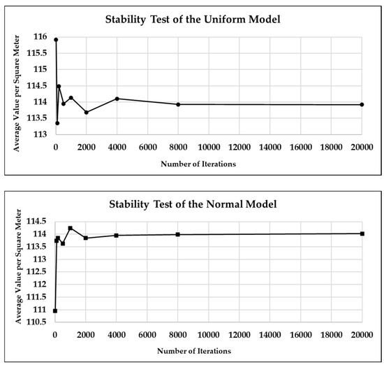
Figure 6.
Stability test for Uniform (top) and Normal (bottom) models.
As shown in Figure 6, the average unit TV in both models fluctuates within a narrow range, approximately between 113.5 and 116 €/m2 in the Uniform model, and between 111 and 114.5 €/m2 in the Normal model. These results indicate that the two models display consistent behavior, with minimal variation as the number of iterations increases.
Furthermore, both models demonstrate clear convergence and satisfactory stability after approximately 4000 Monte Carlo simulations. This confirms that the full set of 20,000 simulations conducted in this study is sufficient to ensure statistical robustness and model reliability. The models can therefore be considered stable and reliable for use in urban transformation feasibility assessments under uncertainty.
It is worth noting that, despite the advantages of this methodology, some limitations still remain. Indeed, the study relies on assumptions regarding input distributions and economic conditions, which may vary depending on regional market dynamics, policy changes, or unforeseen economic shifts. Accordingly, future research should explore hybrid modeling approaches, integrating environmental, social, and economic sustainability indicators to provide a comprehensive assessment of urban transformations.
4. Conclusions
This study investigated the feasibility of urban transformations in three Italian case studies by evaluating the balance between public and private interests through a probabilistic modeling approach based on the MC method. The primary objective was to assess whether such transformation projects can achieve economic sustainability for private developers while simultaneously delivering social and environmental benefits through appropriate urban planning regulations established by public authorities.
The results demonstrated that the MC method is an effective tool for evaluating the TV of urban areas under uncertainty. It provides robust insights into investment feasibility and associated risks.
Among the two models tested, the Uniform distribution yields more dispersed estimates due to broader variability in inputs, making it particularly suitable when there is high uncertainty surrounding key parameters—such as construction costs, market values, or project duration. Conversely, the Normal distribution produces more concentrated estimates around the mean, and is more appropriate when the investment scenario is better defined and data are available.
Beyond the technical comparison of probabilistic distributions, the broader contribution of this work lies in demonstrating how such models can support both public and private stakeholders in navigating complex urban regeneration scenarios. For public institutions, it could be used as a method for calibrating the urban planning parameters listed in each regulatory document, with the aim of guiding private developers toward proposals that not only ensure a reasonable return on investment, but also include the dedication of a portion of land to the public for the creation of high-quality public spaces, such as green areas, parking lots, and other infrastructure that enhances urban ecosystem services. For private investors, once urban planning indices have been defined, this approach could serve as a useful tool for risk analysis, allowing for the evaluation of the likelihood of achieving both favorable and unfavorable investment scenarios.
By explicitly addressing the trade-off between public goals and private profitability, the proposed approach facilitates negotiation and decision-making, especially within the context of PPPs. These collaborative arrangements are increasingly central to urban development policy, and the use of quantitative models can enhance transparency in value-sharing, thus reducing the risk of asymmetries in outcomes.
However, it is important to recognize that the model currently focuses primarily on economic parameters. While the relevance of ecosystem services and sustainability is acknowledged, future research should aim to integrate multi-criteria decision-making tools, Social Return on Investment, or environmental performance indicators, to provide a more holistic assessment of transformation impacts. Furthermore, empirical validation of the model against real-world cases represents another important avenue for future work. This would be feasible once the examined areas are subject to actual transformation and relevant data become available.
To wrap up, under uncertain market conditions, probabilistic models could offer substantial support in balancing public and private interests and guiding investment decisions. The findings of this study suggest that MC-based probabilistic modeling can serve as a powerful decision-support tool within public–private negotiation processes. By grounding urban planning decisions in quantifiable and transparent outcomes rather than arbitrary or rigid regulations, this approach has the potential to reduce conflict and foster more sustainable and balanced urban transformations.
Author Contributions
N.F.: Conceptualization, Data Curation, Formal Analysis, Investigation, Methodology, Resources, Software, Supervision, Validation, Visualization, Writing—Original Draft, Writing—Review and Editing. M.M.: Conceptualization, Data Curation, Formal Analysis, Investigation, Resources, Software, Visualization, Writing—Original Draft. M.R.: Conceptualization, Methodology, Project Administration, Resources, Supervision, Validation, Writing—Review and Editing. All authors have read and agreed to the published version of the manuscript.
Funding
This research received no external funding.
Institutional Review Board Statement
Not applicable.
Informed Consent Statement
Not applicable.
Data Availability Statement
Data used in the present study and the link to download information on case studies have been provided within Section 2.
Conflicts of Interest
The authors declare no conflicts of interest.
References
- Manganelli, B.; Murgante, B. The Dynamics of Urban Land Rent in Italian Regional Capital Cities. Land 2017, 6, 54. [Google Scholar] [CrossRef]
- Berto, R.; Cechet, G.; Stival, C.A.; Rosato, P. Affordable Housing vs. Urban Land Rent in Widespread Settlement Areas. Sustainability 2020, 12, 3129. [Google Scholar] [CrossRef]
- Zhou, M. An interval fuzzy chance-constrained programming model for sustainable urban land-use planning and land use policy analysis. Land Use Policy 2015, 42, 479–491. [Google Scholar] [CrossRef]
- Lu, X.-H.; Ke, S.-G. Evaluating the effectiveness of sustainable urban land use in China from the perspective of sustainable urbanization. Habitat Int. 2018, 77, 90–98. [Google Scholar] [CrossRef]
- Deng, S. Exploring the relationship between new-type urbanization and sustainable urban land use: Evidence from prefecture-level cities in China. Sustain. Comput. Inform. Syst. 2021, 30, 100446. [Google Scholar] [CrossRef]
- Tan, R.; Zhang, T.; Liu, D.; Xu, H. How will innovation-driven development policy affect sustainable urban land use: Evidence from 230 Chinese cities. Sustain. Cities Soc. 2021, 72, 103021. [Google Scholar] [CrossRef]
- Beretić, N.; Talu, V. Social Housing as an Experimental Approach to the Sustainable Regeneration of Historic City Centers: An Ongoing Study of Sassari City, Italy. Sustainability 2020, 12, 4579. [Google Scholar] [CrossRef]
- La Rosa, D.; Privitera, R.; Barbarossa, L.; La Greca, P. Assessing spatial benefits of urban regeneration programs in a highly vulnerable urban context: A case study in Catania, Italy. Landsc. Urban Plan. 2017, 157, 180–192. [Google Scholar] [CrossRef]
- Pantaloni, M.; Marinelli, G.; Santilocchi, R.; Minelli, A.; Neri, D. Sustainable Management Practices for Urban Green Spaces to Support Green Infrastructure: An Italian Case Study. Sustainability 2022, 14, 4243. [Google Scholar] [CrossRef]
- Antoniol, M. Gli Indici Di Edificabilità—Superfici, Volumi e Densità Edilizia; Exeo Edizioni: Padova, Italy, 2011. [Google Scholar]
- Sun, G.; Chen, X.; Jia, X.; Yao, Y.; Wang, Z. Combinational Build-Up Index (CBI) for Effective Impervious Surface Mapping in Urban Areas. IEEE J. Sel. Top. Appl. Earth Obs. Remote. Sens. 2016, 9, 2081–2092. [Google Scholar] [CrossRef]
- Da Silva, F.T.; Reis, N.C.; Santos, J.M.; Goulart, E.V.; de Alvarez, C.E. Influence of urban form on air quality: The combined effect of block typology and urban planning indices on city breathability. Sci. Total. Environ. 2022, 814, 152670. [Google Scholar] [CrossRef] [PubMed]
- Silva, I.; Santos, R.; Lopes, A.; Araújo, V. Morphological Indices as Urban Planning Tools in Northeastern Brazil. Sustainability 2018, 10, 4358. [Google Scholar] [CrossRef]
- Candian, A. Il Contratto Di Trasferimento Di Volumetria; Giuffrè: Rome, Italy, 1990; Volume 62. [Google Scholar]
- Fiorentini, N.; Mariotti, D.; Rovai, M. Defining Risk Curves in feasibility analyses of urban regeneration projects with Monte Carlo method. Valori Valutazioni 2024, 36, 149–170. [Google Scholar] [CrossRef]
- Losasso, M. Urban Regeneration: Innovative Perspectives. Techne J. Technol. Archit. Environ. 2015, 10, 4–5. [Google Scholar]
- Yu, J.-H.; Kwon, H.-R. Critical success factors for urban regeneration projects in Korea. Int. J. Proj. Manag. 2011, 29, 889–899. [Google Scholar] [CrossRef]
- Romanelli, M.; Ferrara, M.; Metallo, C.; Reina, R.; Varriale, L.; Ventura, M.; Vesperi, W.; Buonocore, F. Advancing Urban Regeneration Projects for Sustainable Development and Intellectual Capital. In Proceedings of the European Conference on Knowledge Management, ECKM, Naples, Italy, 1–2 September 2022; Volume 23. [Google Scholar]
- Dell’ovo, M.; Bassani, S.; Stefanina, G.; Oppio, A. Memories at Risk. How to Support Decisions about Abandoned Industrial Heritage Regeneration. Valori Valutazioni 2020, 2020, 107–115. [Google Scholar]
- Abatecola, G.; Mari, M.; Poggesi, S. How Can Virtuous Real Estate Public-Private Partnerships Be Developed? Towards a Co-Evolutionary Perspective. Cities 2020, 107, 102896. [Google Scholar] [CrossRef]
- Guarini, M.R.; Morano, P.; Micheli, A.; Sica, F. Public-Private Negotiation of the Increase in Land or Property Value by Urban Variant: An Analytical Approach Tested on a Case of Real Estate Development. Sustainability 2021, 13, 10958. [Google Scholar] [CrossRef]
- Guarini, M.R.; Morano, P.; Micheli, A. A Procedure to Evaluate the Extra-Charge of Urbanization. In Computational Science and Its Applications—ICCSA 2020, Proceedings of the 20th International Conference, Cagliari, Italy, 1–4 July 2020; Lecture Notes in Computer Science (Including Subseries Lecture Notes in Artificial Intelligence and Lecture Notes in Bioinformatics); Springer: Cham, Switzerland, 2020; Volume 12251 LNCS. [Google Scholar]
- Oppio, A.; Torrieri, F.; Dell’Oca, E. Land Value in Urban Development Agreements: Methodological Perspectives and Opera-tional Recommendations. Valori Valutazioni 2018, 2018, 87–96. [Google Scholar]
- Read, D.C.; Leland, S.; Pope, J. Views from the Field: Economic Development Practitioners’ Perceptions About Public-Private Real Estate Partnerships. Urban Aff. Rev. 2020, 56, 1876–1900. [Google Scholar] [CrossRef]
- Soriano Llobera, J.M.; Roig Hernando, J. Public-Private Partnerships for Real Estate Projects: Current Framework and New Trends. Reg. Sect. Econ. Stud. 2015, 15, 35–44. [Google Scholar]
- Morano, P.; Tajani, F.; Anelli, D. Urban Planning Variants: A Model for the Division of the Activated “Plusvalue” between Public and Private Subjects. Valori Valutazioni 2021, 28, 31–47. [Google Scholar] [CrossRef]
- Ragazzo, M. Il Cambio Di Destinazione d’uso e Il Pagamento Del Contributo per Oneri Di Urbanizzazione. Urban. Appalti 2005, 10, 1201–1210. [Google Scholar]
- D’Amato, M.; Cvorovich, V.; Amoruso, P. Short Tab Market Comparison Approach. An Application to the Residential Real Estate Market in Bari. In Studies in Systems, Decision and Control; Springer: Cham, Switzerland, 2017; Volume 86. [Google Scholar]
- Del Territorio, A. Manuale Operativo Delle Stime Immobiliari; FrancoAngeli: Milan, Italy, 2011; Volume 17. [Google Scholar]
- Zhai, B.; Chen, H.; Chen, A. Study on Investment Risk Assessment Model of Real Estate Project Based on Monte Carlo Method. In IOP Conference Series: Earth and Environmental Science; IOP Publishing: Bristol, England, 2018; Volume 189. [Google Scholar]
- Mangialardo, A.; Micelli, E. Simulation Models to Evaluate the Value Creation of the Grass-Roots Participation in the Enhancement of Public Real-Estate Assets with Evidence from Italy. Buildings 2017, 7, 100. [Google Scholar] [CrossRef]
- Bao, H.; Chong, A.Y.-L.; Wang, H.; Wang, L.; Huang, Y. Quantitative decision making in land banking: A Monte Carlo simulation for China’s real estate developers. Int. J. Strat. Prop. Manag. 2012, 16, 355–369. [Google Scholar] [CrossRef]
- Barañano, A.; De La Peña, J.I.; Moreno, R. Valuation of real-estate losses via Monte Carlo simulation. Econ. Res. Ekon. Istraz. 2020, 33, 1867–1888. [Google Scholar] [CrossRef]
- Del Giudice, V.; De Paola, P.; Forte, F.; Manganelli, B. Real Estate Appraisals with Bayesian Approach and Markov Chain Hybrid Monte Carlo Method: An Application to a Central Urban Area of Naples. Sustainability 2017, 9, 2138. [Google Scholar] [CrossRef]
- Hoesli, M.; Jani, E.; Bender, A. Monte Carlo simulations for real estate valuation. J. Prop. Invest. Finance 2006, 24, 102–122. [Google Scholar] [CrossRef]
- Loizou, P.; French, N. Risk and Uncertainty in Development: A Critical Evaluation of Using the Monte Carlo Simulation Method as a Decision Tool in Real Estate Development Projects. J. Prop. Invest. Financ. 2012, 30, 198–210. [Google Scholar] [CrossRef]
- Amar, J. The Monte Carlo method in science and engineering. Comput. Sci. Eng. 2006, 8, 9–19. [Google Scholar] [CrossRef]
- The European Parliament and the Council of the European Union. Regulation (EU) No 575/2013 of 26 June 2013 on Prudential Requirements for Credit Institutions and Investment Firms and Amending Regulation (EU) No 648/2012; EUR-lex: Brussels, Belgium, 2013. [Google Scholar]
- Collegio degli Ingegneri e Architetti di Milano Prezzi Tipologie Edilizie. DEI S.R.L. Tipografia del Genio Civile, Roma; Gruppo LSWR: Milan, Italy, 2024. [Google Scholar]
- Ministero per i Lavori Pubblici. Decreto Ministeriale 2 Aprile 1968: Limiti Inderogabili Di Densità Edilizia, Di Altezza, Di Distanza Fra i Fabbricanti e Rapporti Massimi Tra Spazi Destinati Agli Insediamenti Residenziali e Produttivi e Spazi Pubblici o Riservati Alle Attività Collettive, al Verde Pubblico o a Parcheggi Da Osservare Ai Fini Della Formazione Dei Nuovi Strumenti Urbanistici o Della Revisione Di Quelli Esistenti, Ai Sensi Dell’art. 17 Della Legge 6 Agosto 1967, n.765; 1968. Available online: https://www.gazzettaufficiale.it/eli/id/1968/04/16/1288Q004/sg (accessed on 24 April 2025).
- Comitato di Basilea per la Vigilanza Bancaria. Convergenza Internazionale Della Misurazione Del Capitale e Dei Coefficienti Patrimoniali; Nuovi Schemi Di Regolamentazione; Bank for International Settlements: Basel, Switzerland, 2004. [Google Scholar]
- Ministero per i Lavori Pubblici. Legge 24 Marzo 1989, n. 122: Disposizioni in Materia Di Parcheggi, Programma Triennale per Le Aree Urbane Maggiormente Popolate, Nonché Modificazioni Di Alcune Norme Del Testo Unico Sulla Disciplina Della Circolazione Stradale, Approvato Con Decreto Del Presidente Della Repubblica 15 Giugno 1959, n. 393.; 1989. Available online: https://www.normattiva.it/uri-res/N2Ls?urn:nir:stato:legge:1989-03-24;122 (accessed on 24 April 2025).


Disclaimer/Publisher’s Note: The statements, opinions and data contained in all publications are solely those of the individual author(s) and contributor(s) and not of MDPI and/or the editor(s). MDPI and/or the editor(s) disclaim responsibility for any injury to people or property resulting from any ideas, methods, instructions or products referred to in the content. |
© 2025 by the authors. Licensee MDPI, Basel, Switzerland. This article is an open access article distributed under the terms and conditions of the Creative Commons Attribution (CC BY) license (https://creativecommons.org/licenses/by/4.0/).