AI-Aided GPR Data Multipath Summation Using x-t Stacking Weights

Abstract

The Ground Penetrating Radar (GPR) method can image dielectric discontinuities in subsurface structures, which cause the reflection of electromagnetic (EM) waves. These discontinuities are imaged as reflectors in GPR sections, often distorted by diffracted energy. To focus the diffracted energy within the GPR sections, migration is commonly used. The migration velocity of GPR data is a low-wavenumber attribute crucial for effective migration. Obtaining a migration velocity model, typically close to a Root Mean Square (RMS) model, from zero-offset (ZO) data requires analysis of the available diffractions, whose density and (x, t) coverage are random. Thus, the accuracy and efficiency of such a velocity model, whether for migration or interval velocity model estimation, are not guaranteed. An alternative is the multipath summation method, which involves the weighted stacking of constant velocity migrated sections. Each stacked section contributes to the final stack, weighted by a scalar value dependent on the constant velocity value used and its relation to its estimated mean velocity of the section. This method effectively focuses the GPR diffractions in the presence of low heterogeneity. However, when the EM velocity varies dramatically, 2D weights are needed. In this study, with the aid of an Artificial Intelligence (AI) algorithm that detects diffractions and uses their kinematic information, we generate a diffraction velocity model. This model is then used to assign 2D weights for the weighted multipath summation, aiming to focus the scattered energy within the GPR section. We describe this methodology and demonstrate its application in enhancing the lateral continuity of reflections. We compare it with the 1D multipath summation using simulated data and present its application on marble assessment GPR data for imaging cracks and discontinuities in the subsurface structure.

1. Introduction

The main aim of the Ground Penetrating Radar (GPR) method is to represent the dielectric inhomogeneities for the interpretation of GPR sections. The dielectric inhomogeneities cause the EM (electromagnetic) signal, transmitted by the GPR transmitter, to reflect back to the surface, where it is recorded by the GPR receiver. GPR sections are often dominated by scattered energy due to the gradual variation in moisture or weak reflectivity, together with the high resolution of the GPR frequencies [1]. In this way, the coherent signal is masked, biasing the interpretation.

The migration of GPR data is an image processing technique which gathers the energy of diffractions and positions the energy of reflections to the correct location on the x-t or the x-z plane. It was observed by ref. [1] that diffractions, when migrated with the correct velocity, collapse to their apices, which means that after migration they can be treated as a coherent signal [2]. Velocity analysis is crucial for effective migration. Obtaining effective EM velocity models has been implemented for GPR studies, following the seismic reflection method sequence, which requires multi-offset data and velocity picking over semblance maps [3,4]. This can be circumvented by using average velocities, core studies, or other knowledge for the subsurface conditions, as well as diffraction hyperbola kinematic characteristic studies [4,5,6,7]. The latter can follow hyperbola fitting [8,9] or multi-focusing methods.

Multi-focusing methods apply a number of constant velocity migrations to estimate focusing attributes like kurtosis [10,11] or local slopes of the wavefield [12,13]. The focusing attribute obtains an extremum for a specific EM velocity value. This attribute can be used in two ways: (1) to estimate a migration velocity model for migration [11,14], or (2) for constant velocity migrated section-weighted stacking (multipath summation) to achieve direct focusing without a velocity model [12,13,15].

The latter approach requires the user to define a pre-determined EM velocity range. It also involves applying plane wave destruction (PWD) filters to evaluate diffraction focusing. This evaluation is based on the standard deviation of the local slopes of each constant velocity migration section. These sections are then used for the multipath summation final stacking. The standard deviation of the migrated section’s local slopes is used for the estimation of stacking weights. The relatively large number of migrations needed, followed by time-varying spectral whitening methods for de-blurring, increases the computational cost. It appears that the key to both reducing the computational cost and improving the effectiveness of the multipath summation is to reduce the number of migrations [13]. This can be achieved by introducing more sophisticated local weights within the x-t plane, instead of using a weight for the entire section.

We propose and apply 2D-weighted constant velocity migrated GPR section stacking to produce a time migrated multi-focused GPR section. With the aid of Artificial Intelligence (AI), diffractions are adaptively localized for the estimation of a “diffraction velocity model”. Even though this kind of velocity model is commonly used for migration, it is often far from an efficient migration velocity model. Here, we demonstrate that a diffraction velocity model can be sufficient for generating 2D weights, with which each constant velocity migrated section contributes to the final stack. We demonstrate the effectiveness of the method on synthetic GPR data and data acquired over a quarry for imaging cracks and voids within marble volumes.

2. Materials and Methods

The hyperbola branches of a GPR diffraction move in the x-t domain after migration, but the apex remains stationary (Figure 1) [12]. Stacking of a constant velocity migrated diffraction can theoretically cancel the hyperbola branches and enhance the hyperbola apex in a continuous world. However, the discrete number of velocities used for constant velocity migrations results in incomplete cancelation of the branches, which contaminates and blurs the signal [11].

To suppress the diffraction tails and limit the blurriness of the outcome, a weighted summation was implemented by refs. [12,15] using 1D weights. To recover temporal resolution, ref. [12] proposed a time-varying post-multipath summation step. The constraint of the migration velocity range used in multipath summation and the reduction in the user interference was implemented by ref. [13]. Here, we propose a method to reduce the number of migrations needed. The method aims to avoid blurriness and effectively focus the scattered energy of the entire GPR section through an adaptive scheme [7,16].

If A(x, t) is a GPR section and Am(x, t, u) is the migrated GPR section using a constant velocity value u, then a non-weighted multipath summation section B(x, t, u₁, u₂) can be expressed as follows:

$$B\left(x,t,u_1,u_2\right)={\displaystyle \frac{1}{{\int }_{u_1}^{u_2}G\left(u\right)du}}{\int }_{u_1}^{u_2}{A}_m\left(x,t,u\right)du$$

(1)

where u₁ and u₂ are the limits of the velocity range used for constant velocity migrations. If G(u) is a Gaussian function with its maximum equal to unity at the velocity mean value, and if other velocities are assigned a weighting factor increasing closer to the vicinity of this mean value, then a weighted multipath-way summation section can be expressed as follows:

$$B(x,t,u_1,u_2)={\displaystyle \frac{1}{{\int }_{u_1}^{u_2}G\left(u\right)du}}{\int }_{u_1}^{u_2}{A}_m(x,t,u)G(u)du$$

(2)

The G(u_n) factor follows a 1D Gaussian distribution with its maximum at the mean velocity value of the u_n velocity range used. Here, we propose a 2D weighting function, G(x, t, u).

$$(x,t,u_1,u_2)={\displaystyle \frac{1}{{\int }_{u_1}^{u_2}G(x,t,u)du}}{\int }_{u_1}^{u_2}{A}_m(x,t,u)\odot G(x,t,u)du$$

(3)

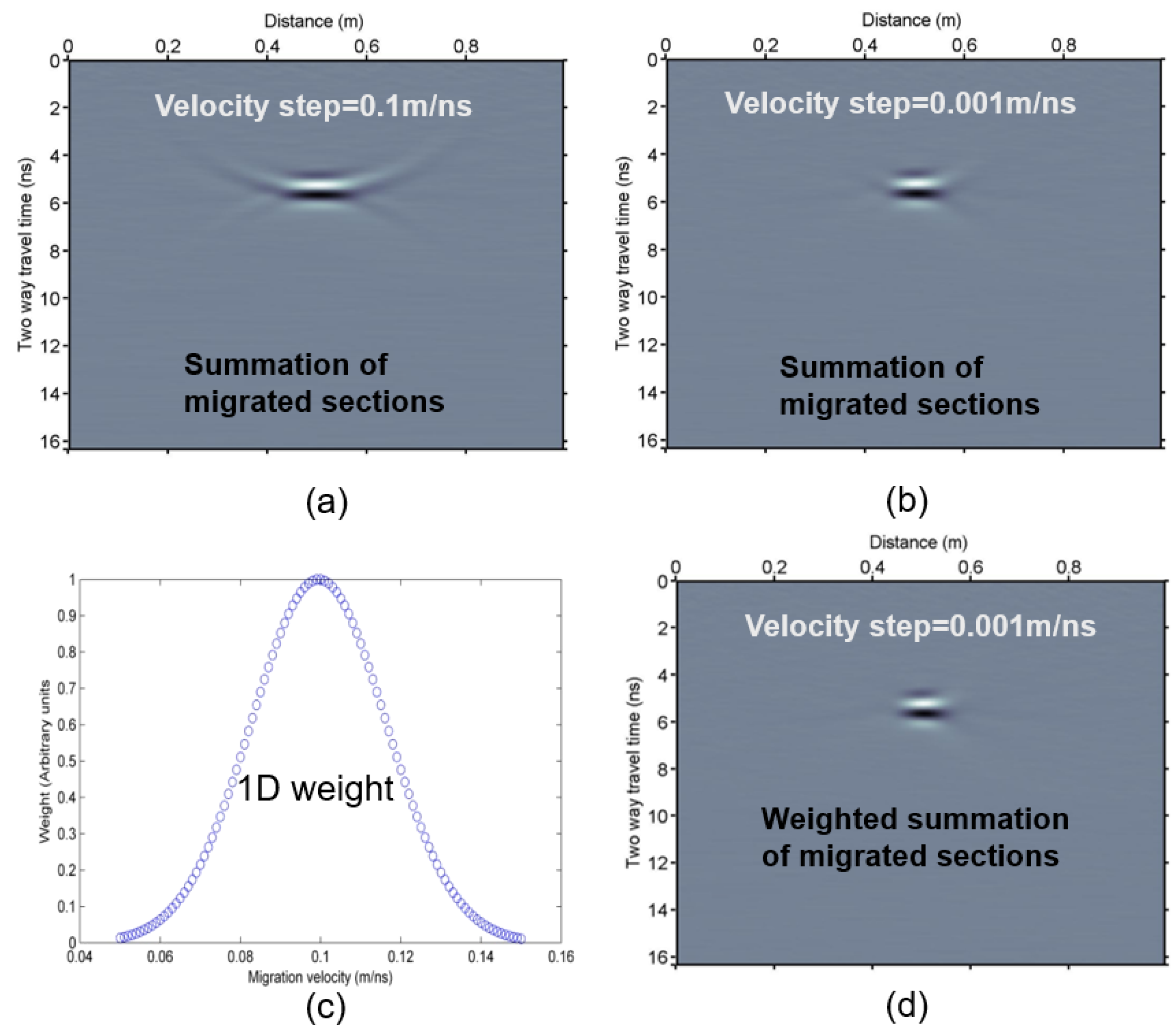
where $\odot$ is a Hadamard operator. To demonstrate the usefulness of the need for many migrations and summation weights, we used Equation (1) on the section depicted in Figure 1a, using a velocity range from 0.05 m/ns up to 0.15 m/ns with a velocity step of 0.1 m/ns. We migrated this section with a constant velocity using each one of the values of this range and then summed the sections (Equation (1), Figure 2a). The stacked section depicted gathered energy around the hyperbola apex, but tails are not canceled. With the usage of a larger number of migrations, using a step of 0.001 m/ns, the tails are more suppressed (Figure 2b). Using a Gaussian weight for each one of the migrated sections used in the final stack, according to Figure 2c, the final stack’s energy is even more concentrated to the apex (Equation (2), Figure 2d). Refs. [12,13] proposed methodologies to have a narrower weighting function (more concentrated to the mean velocity, e.g., to 0.1 m/ns in Figure 2c) to reduce the number of migrations. Still, highly heterogeneous EM velocities of the subsurface structure may result in the need for a 2D approach.

The advantage of involving a 2D weighting function (Equation (2)) instead of the 1D formulation (Equation (1)) lies in the fact that we can confront lateral and vertical migration velocity heterogeneity. Additionally, the number of migration operations is reduced. For this, we need an adaptive and low computational cost estimation for the diffraction velocity model, which can be implemented by using AI and further lead to the G(x, t, u) estimation.

The proposed methodology involves the processing steps below:

(1)

Pre-processing of GPR section.

(2)

Machine learning localization and mapping of diffraction hyperbolas.

(3)

Diffraction velocity model estimation.

(4)

Estimation of 2D weights.

(5)

Time migrations with constant velocities u_n.

(6)

Weighting (multiplication) of each one of the migrated GPR sections.

(7)

Stacking (summation) of all weighted time migrated GPR sections.

Step 1 includes conventional processing: Dewow, suppression of semi- and fully horizontal reflectors using mean traces of narrow x-distances and band-pass filtering. Since this step is just before the diffraction localization, the main aim is to enhance the diffractions, which may not be possible with the conventional stages mentioned before. For this, one can also use plane wave destruction (PWD) filters to suppress reflections’ amplitudes [11,12], using the following local plane wave equation:

$${\displaystyle \frac{\partial P}{\partial x}}+\sigma {\displaystyle \frac{\partial P}{\partial t}}=0$$

(4)

where P stands for the wavefield, σ the local slope, and x and t the space and time variables. A modification of the C3 algorithm includes delineating connected clusters on neighboring traces and hyperbola fitting (step 2) [7,16], as well as straight line fitting of the hyperbola x²−t² image coordinates (step 3). This step concludes with the interpolation of the hyperbola apex points, which were assigned a specific EM velocity value. The hyperbola can be described as follows:

$$t^2=t_0^2+{\left({\displaystyle \frac{2}{v}}\right)}^2{\mathrm{x}}^2$$

(5)

where t is the two-way travel time, x is the distance from the apex of the diffraction at x₀ to an arbitrary distance, v the EM propagation velocity, and t₀ is the two-way travel time at x₀. The factor (2/v)² is the slope of the straight line over x²−t² coordinates.

The velocity estimated based on the above is considered as the Root Mean Square (RMS) velocity, and it is commonly used for migration. This way of acquiring a velocity model, although efficient for diffraction focusing, mathematically depends heavily on the density of the estimations within the x-t plane, which are based on the number of located hyperbolas. Therefore, this velocity model is not guaranteed to be efficient for migration. This kind of velocity model, which we prefer to name as a diffraction velocity model, and its velocity range can be effectively used for focusing the localized diffraction energy, and thus for 2D weight estimation (step 4).

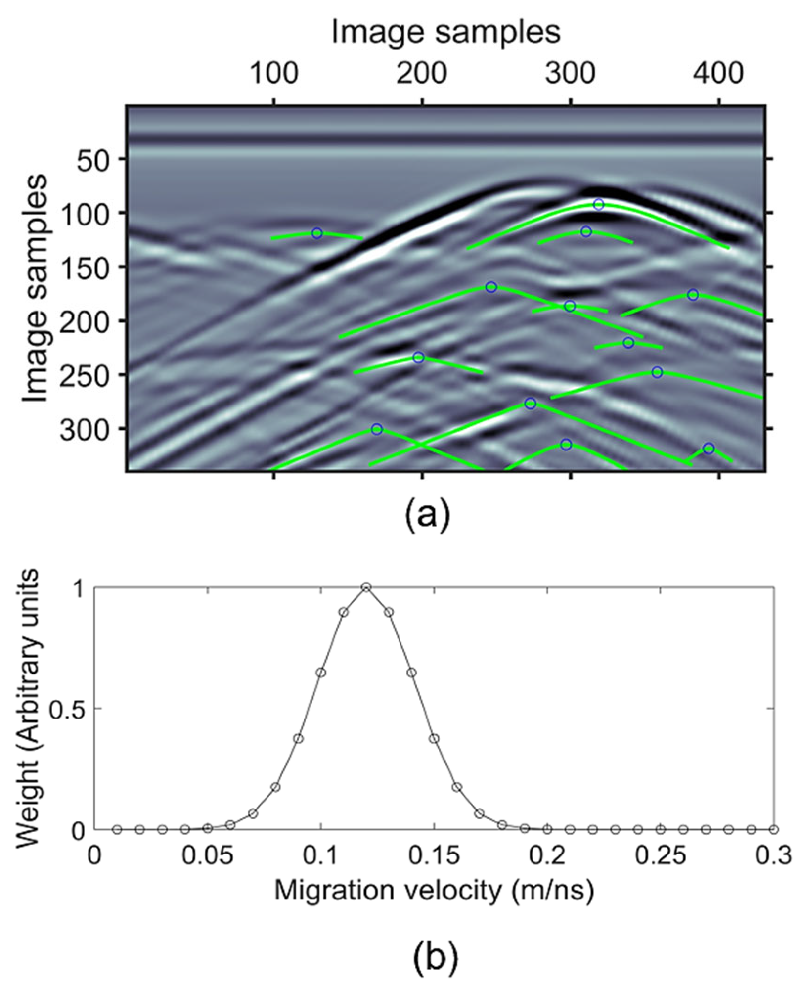
The 2D weight values are based on a 1D weight vector of global velocity range 0.04 m/ns–0.3 m/ns. Each velocity within the estimated migration velocity model corresponds to a weight on this vector, and its (x, t) point in the 2D weight plane is assigned with this weight value. The Hadamard product, or element-wise product, of a constant velocity migrated section of 0.12 m/ns and the corresponding 2D weight matrix remains a migrated section with a constant velocity model of 0.12 m/ns, but x-t points with this velocity value in the estimated diffraction velocity model (i.e., diffractions characterized by 0.12 m/ns velocity have been located at these points) are enhanced while smoothly degrading the rest of the section’s amplitudes. This is not the case for 1D weights [13], which favor only the parts of the multipath summation section with hyperbolas’ kinematic characteristics close to the user-defined mean velocity value of the whole section. Note in Figure 4b that the weights, only close to the vicinity of the maximum value, have a sufficient contribution to the stack, avoiding in this way an increased blurriness in the outcome. The same procedure is followed for each one of the velocities in a chosen range. Even though an initial velocity range is chosen at step 2, this is updated from the extreme velocity values in the estimated diffraction velocity model of step 3. The step for migrations is 0.01 m/ns. Sequential constant velocity migrations and weighted summation (steps 5 and 6), followed by a final Hadamard multiplication with the inverse values sum of all 2D weights (Equation (3)), conclude to a focused multipath summation GPR section. Here, for migration, we use the F-K migration method.

3. Results

3.1. Synthetic Example

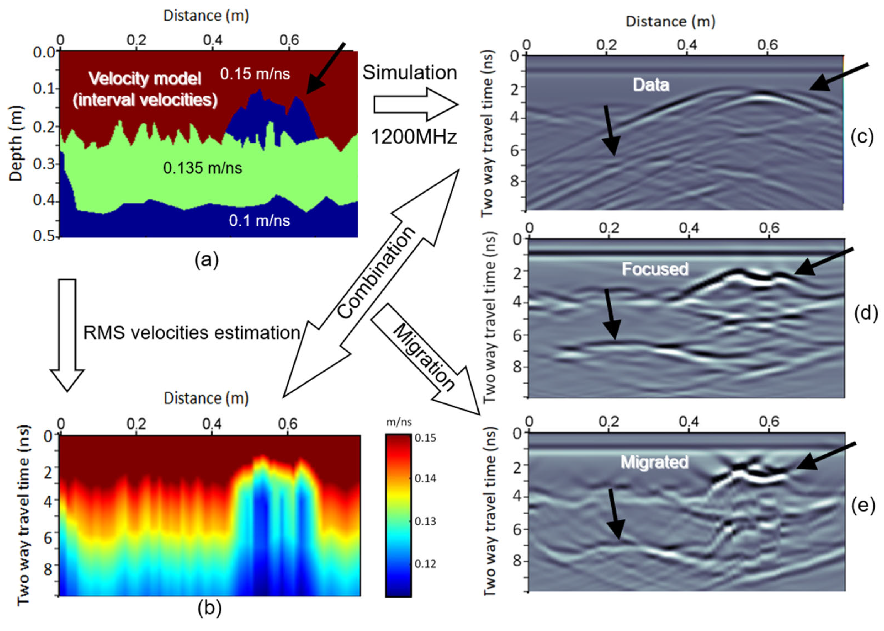
We simulated a zero-offset transmitter–receiver measurement setup with an antenna of 1200 MHz dominant frequency over a buried structure with EM velocity variation as illustrated in Figure 3a [13]. Three main layers are visible, with a narrow low velocity intrusion within the first layer, which are characterized by an RMS velocity model as depicted in Figure 3b. We used a finite difference grid of 0.005 ns × 0.0005 m to generate a GPR section, which was then resampled with distance and time intervals of 0.01 m and 0.05 ns, respectively (Figure 3c). The GPR section lacks visual reflection information, but rather shows a large amount of scattered energy. The pre-processing stage was not needed here. The RMS velocity model was combined with the GPR section in a Kirchhoff migration algorithm to produce a migrated section with the assumption that the Earth’s dielectric variation is known (Figure 3d).

Under the 1D multipath summation formulation [12,13], we used the local slopes of each constant velocity migrated section within a velocity range of 0.05 m/ns to 0.19 m/ns (Figure 4b, using the weights which have a non-zero contribution to the stack), using 26 migrations for the evaluation of the 1D Gaussian weighting function. After the weighted stacking (Equation (2)) of the migrated sections, we obtained the focused GPR section in Figure 3e.

Black arrows indicate two areas of interest which can be the basis for the methodology’s performance. The upper right arrows in Figure 3a,c demonstrate the inability of the raw data to image the rough interface of the shallow high velocity layer and the lower velocity narrow layer, which also suggests that a focusing method is required. For this, the multipath summation focused the certain interface (Figure 3d). It does not perfectly correct the large slopes (comparison of Figure 3a,d), but it images a smooth laterally varying interface. Phase differences at around 0.6 m from the beginning of the study line and at around 3 ns are observed. This area images the contribution of two strong diffractions, usually not correctly considered as a diffraction also. Migration images this interface more correctly than the multipath summation section in Figure 3d, but it over-migrates the upper part due to the delay of the wavelet (convolutional model), which is within the lower velocity layer; this is a common artifact (Figure 3e). The almost horizontal reflector at around 7 ns is imaged at both sections, with the multipath summation result being more blurred (Figure 3d,e). Still, one must keep in mind that Figure 3e images a migrated section with both homogeneous layers and known velocities, which are both impossible to have in real life.

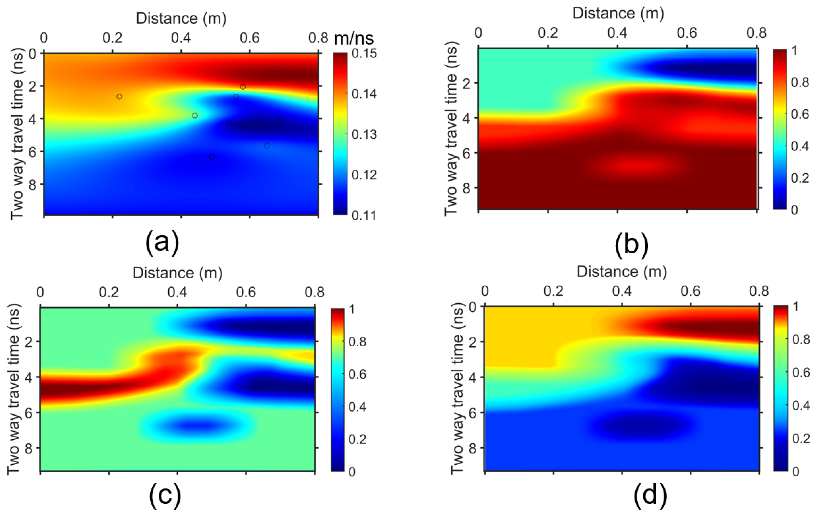
To implement the 2D weighting multipath summation proposed here, we located diffractions within the section after transforming it to a raster image (Figure 4a, i.e., a png image) [7,17]. With the use of Equation (5), we estimated the diffraction velocity model depicted in Figure 5a. The points on which the diffraction velocity model is based are sparse (black circles, Figure 5a). This is due to three main reasons: (1) the detection ability of the machine learning algorithm, (2) the true number of diffractors, and (3) the threshold set. Note the difference between this velocity model and the true RMS velocity model in Figure 3b. The threshold of the velocity range between 0.11 m/ns and 0.15 m/ns was chosen from the velocity range estimated in the diffraction velocity model (Figure 5a).

The number of points used (8 points) is 40% less than the diffractions located by the ML algorithm (13 diffractions). This is indicative of the accuracy of the ML method, which may detect false information, and to avoid this a velocity value threshold should be used. Figure 5b–d depict the representative 2D weights utilized for stacking in the two final steps of the methodology. To explain the generation of the 2D weights described above in the previous section, where Figure 4b was mentioned, the 2D weight matrix in Figure 5c obtained its values by the combination of Figure 4b and Figure 5a. Each value within the velocity model in Figure 5a was assigned a weight based on Figure 4b, and the former was transformed to the 2D or x-t stacking weight depicted in Figure 5c. Figure 5b images the 2D weight of velocity 0.11 m/ns, which has its highest value images in red in areas of Figure 5a imaged in blue color. Similarly, Figure 5c images in red the light blue and green area of 0.13 m/ns in Figure 5a, while Figure 5d is similar to Figure 5a because both have their highest values at 0.15 m/ns.

The migrated section using the estimated diffraction velocity field is far less efficiently focused than the result of the proposed methodology (comparison of Figure 6a,b), which in its turn is similar (but slightly better) to the section obtained by the 1D Gaussian weight methodology (Figure 3d). For the section depicted in Figure 6b, only 7 migrations were estimated, namely for velocity values in the range of 0.09 m/ns–015 m/ns, with a step of 0.01 m/ns, instead of the 26 needed for the section in Figure 3d.

Focusing on the choice of the estimated diffraction velocity model for migration (Figure 6a) or multipath summation using x-t stacking weights (Figure 6b), we could comment on the indications by black arrows. The area indicated on the right of the section is much more blurred in the multipath summation section, but not over-migrated at points as in the migrated section, while the reflector imaging in the lower end of the first velocity layer is relatively evenly imaged by both methods, but the lower end of the second velocity layer is not imaged by the direct migration method, which of course is because at 7 ns the true migration velocity imaged in Figure 3b is 0.13 m/ns, thus this area remains under-migrated in Figure 6a.

3.2. Real Data

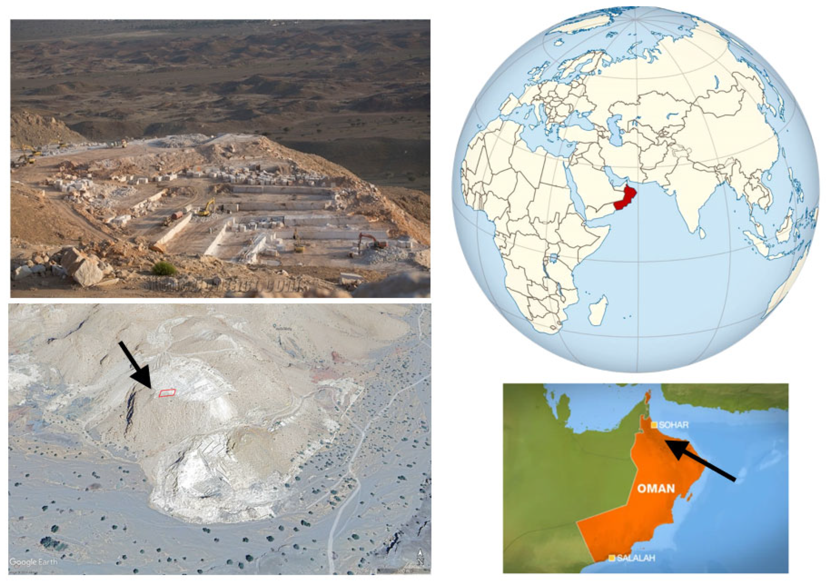
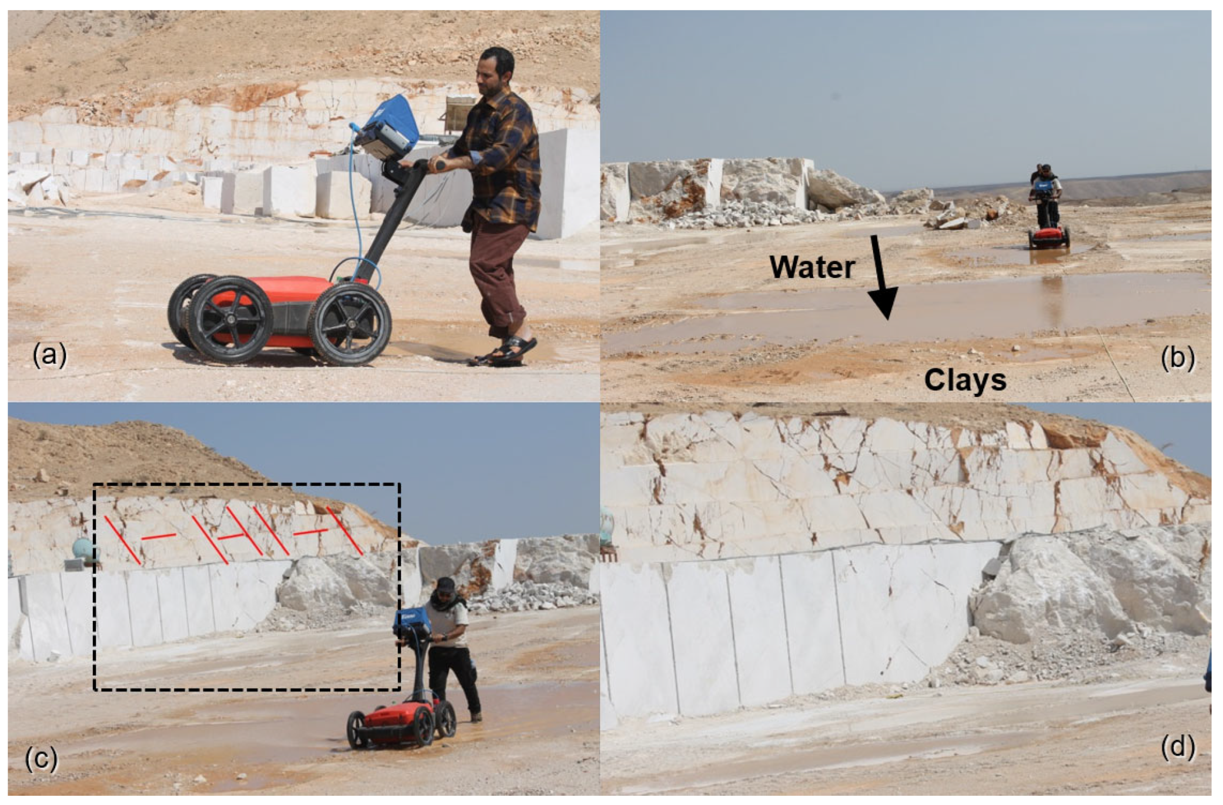
The proposed methodology was applied on a GPR dataset acquired within a marble quarry in Oman, and more specifically at the Sohar Quarry of the Al Ajmi Marble Company in Northern Oman (Figure 7). The scope was to assess the marble volumes by imaging the cracks in stone. It was a pilot study for testing the GPR as a sole method for guiding the marble extraction toward a sustainable quarrying. Forty-one (41) GPR parallel study lines were scanned with an SIR-3000 system (GSSI) equipped with a 400 MHz shielded antenna. The length of the lines was almost 44 m, with a time interval of 0.1378 ns and a space interval of 0.02 m (Figure 8). The area was covered by clays, and there was plenty of water due to both the nearby cutting area and a heavy rain which occurred the day before—a rare phenomenon in Oman which happens once or twice a year (Figure 8b,d). The shallow cracks and their overall orientations were visible within the exposed marble volumes (Figure 8a,c), which guided the GPR survey direction. The survey lines were chosen to be as perpendicular as possible to these cracks.

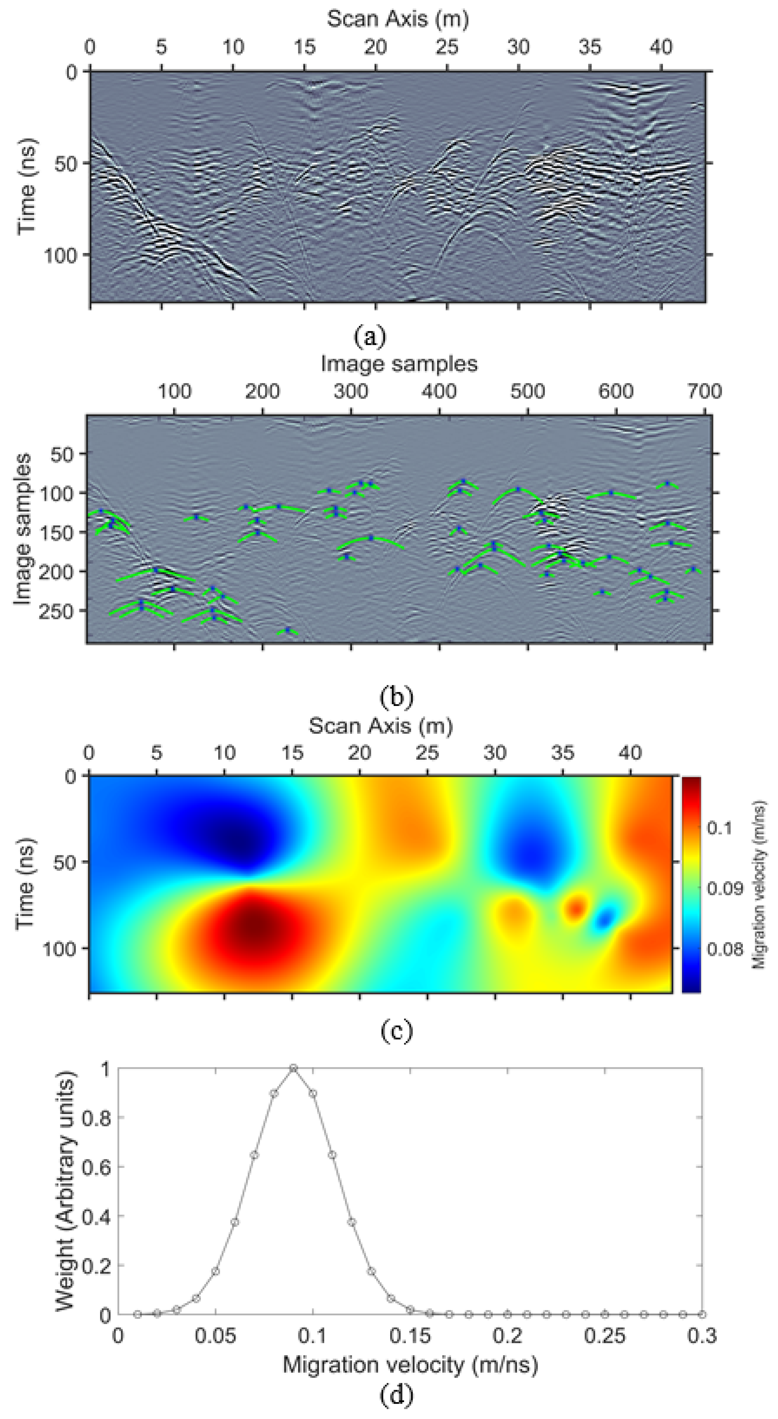
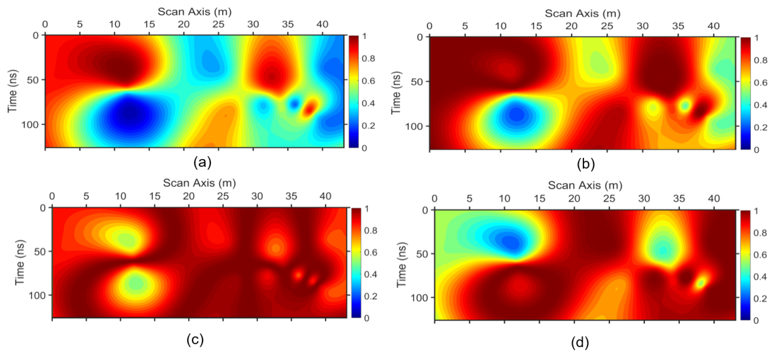
The initial processing included a time-zero shift, Dewow, a background filter of 100 traces, and finally a trapezoid band-pass filtering with edges at 85 MHz-115 MHz-900 MHz-1200 MHz (Figure 9a). The background filter was efficient for the enhancement of the diffracted energy and PWD, based on Equation (4), was not needed here [12]. A machine learning algorithm [7,16] located a number of diffractions (Figure 9b, light green lines) and estimated a diffraction–migration velocity model based on the apex (x, t) points of velocity values within a constrained velocity range of 0.07 m/ns–0.11 m/ns (Figure 9c). This range was chosen for the 2D stacking weights methodology, indicating that the estimated diffraction velocity can serve for the choice of the velocity range to be used for the 2D multipath summation, while for the 1D case several constant velocity migrations and local slope estimations were needed [12]. Indicative 2D weights for the final stacking are depicted in Figure 10. As described in the last paragraph of Section 2, where the methodology is described, the estimation of the 2D weight values is based on 1D weight vectors of the global velocity range 0.01 m/ns–0.3 m/ns (Figure 9d shows an example for the estimation of a 2D weight corresponding to 0.1 m/ns velocity). Each velocity within the estimated migration velocity model corresponds to a weight on this vector and its (x, t) point in the 2D weight plane, and is assigned with this weight value. The Hadamard product of a constant velocity migrated section of 0.1 m/ns and the corresponding 2D weight matrix remains a migrated section with a constant velocity model of 0.1 m/ns, but x-t points with this velocity value in the estimated diffraction velocity model (i.e., diffractions characterized by 0.1 m/ns velocity have been located at these points) are enhanced, while smoothly degrading the rest of the section’s amplitudes. The velocity value of 0.09 m/ns is light blue to light green in Figure 9c. At the same areas in Figure 10c, where the 0.1 m/ns velocity 2D weight is imaged, the aforementioned areas are plotted, with the highest value of 1, in a dark red color, which indicates that this weight favors the areas with diffraction velocity of 0.09 m/ns. Similarly, the 2D weight of 0.1 m/ns velocity (Figure 10d) favors the areas of 0.1 m/ns velocity, which are also imaged in red in Figure 9c, while degrading the others in a smooth way based on a Gaussian function. Note in Figure 9b that the weights, only close to the vicinity of the maximum value, have a sufficient contribution to the stack, avoiding in this way an increased blurriness in the outcome.

We migrated the initially processed dataset depicted in Figure 9a with a constant velocity model of 0.1 m/ns (Figure 11a) after the stacking of 1D- (Figure 11b) and after the stacking of 2D-weighted constant velocity migrations (Figure 11c). Several over-migrated areas are imaged in the former (red arrows) and in the middle (black arrows), even though several other areas are satisfactory focused. A comparison of Figure 11b,c at areas indicated by white arrows demonstrates the efficiency of the 2D stacking weight methodology for focusing on the cracks, which is of the most importance in the present study. This example consists of marble GPR lines with a relatively non-homogeneous velocity, which is most common. Clays, but mostly water from above which intruded on the marble volumes from the cracks, altered the EM velocity in such a way that it is very difficult for migration to perform efficiently. An adaptive scheme for all study lines led to the focused sections, from which two indicative are depicted in Figure 12. The main features are thick cracks, mainly at the shallow (green arrows), arbitrary fractured areas at the shallow (blue arrows) and at deeper positions (black arrows). This is the case for almost all the GPR depth sections, and it can also be observed at depth slices (Figure 13). The healthier rock is considered to be the areas in blue lacking diffractions or signal due to the dielectric contrast, imaged in a dark red color (Figure 13).

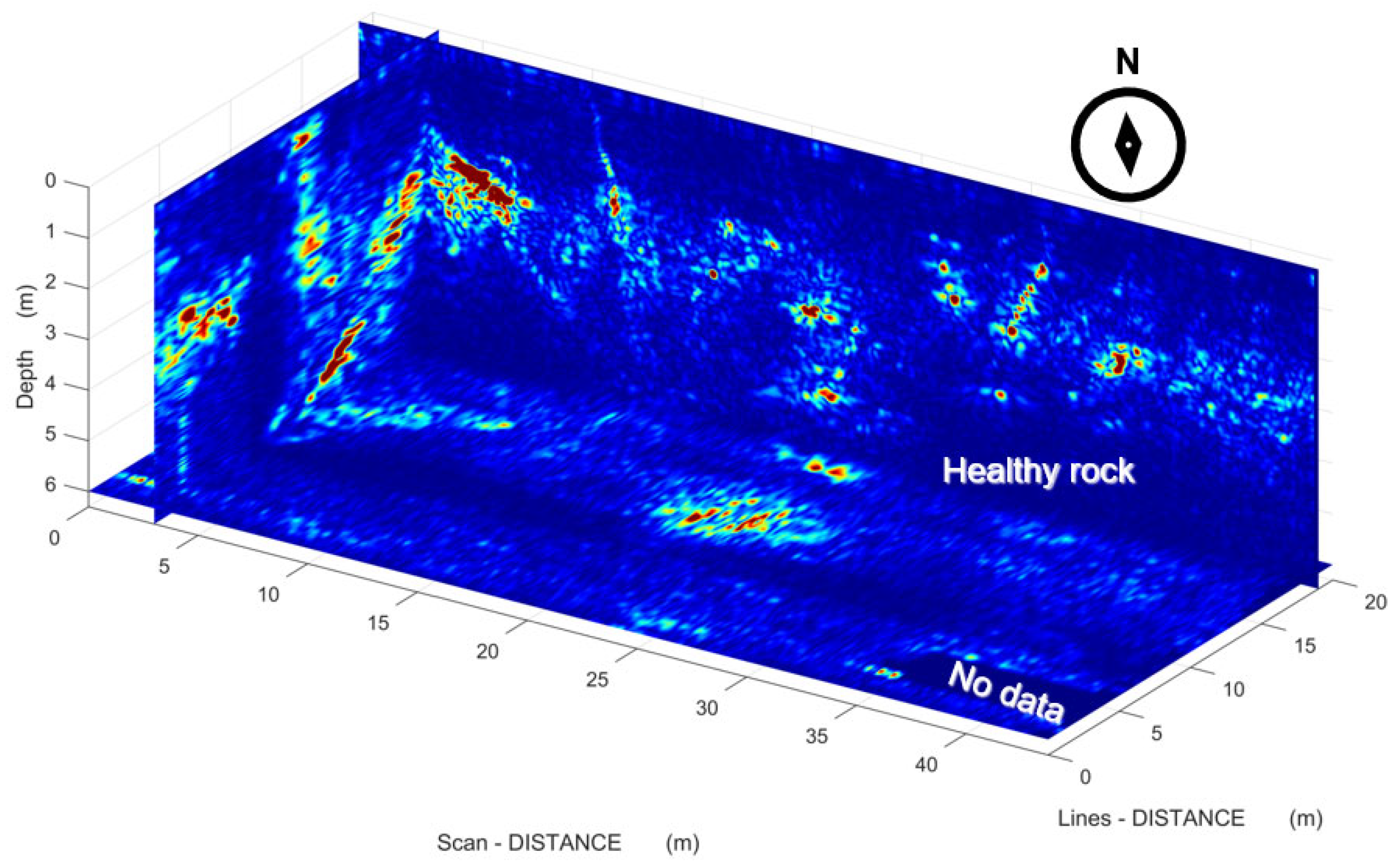
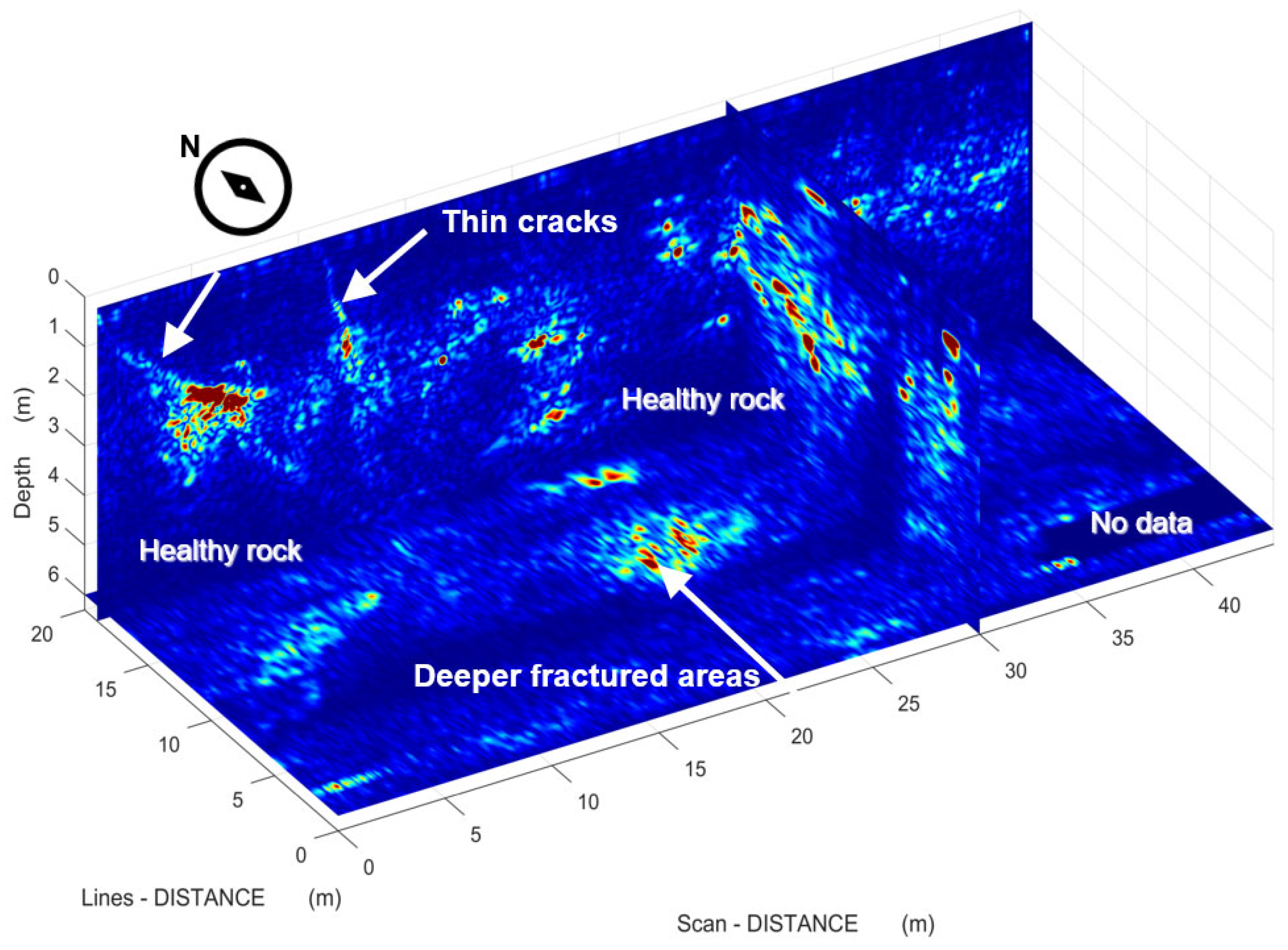
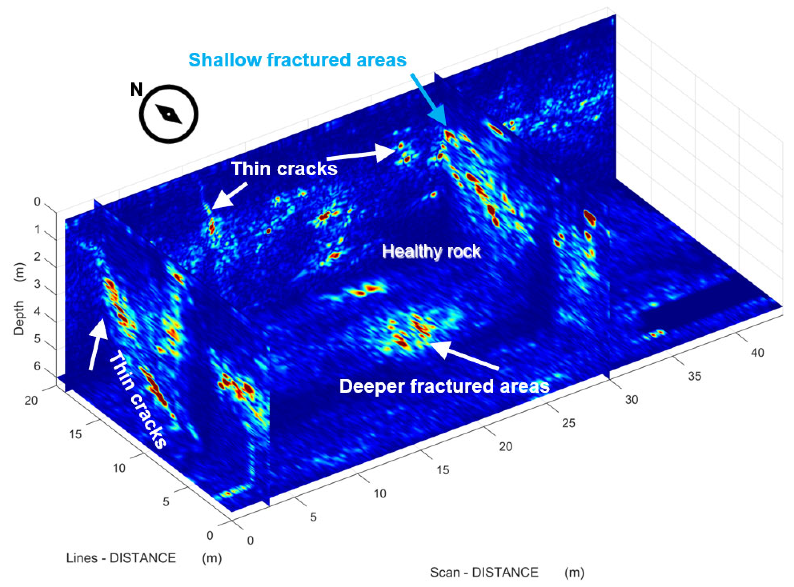
Similarly, one can observe the 3D orientation of the shallow thin cracks (Figure 14, Figure 15 and Figure 16), as well as the deeper fractured areas and the healthy marble volume areas (Figure 15 and Figure 16).

4. Discussion

With the goal of enhancing the resolution of GPR sections for imaging narrow dielectric contrasts like cracks and discontinuities, we developed a methodology based on a novel multipath summation method, which involves 2D stacking weights in the (x, t) plane. The weights, having the same dimensions as the GPR sections, are applied to each section by their Hadamard multiplication, which enhances specific (x, t) areas that are characterized by a specific EM velocity.

An ideal velocity model would focus all the scattered energy efficiently; however, such a model is rarely achievable in practice, as its accuracy depends on the diffraction density across the (x, t) plane. On the other hand, multipath summation focuses each point based on the velocity estimated in the surrounding area, using a series of stacked migrations rather than migrations alone, with the goal of eliminating the hyperbolas’ flanks. As a result, the multipath summation section does not correspond to a specific velocity model, but to a combination of models determined by the 2D weights (Figure 5 and Figure 10).

A comparison of Figure 3d and Figure 6b shows that the 2D weighting methodology provides a slightly better result than the 1D approach. This is evident from the observation that Figure 6b does not emphasize the shallow interface (rightmost black arrow) more than the almost horizontal reflector (leftmost back arrow), as seen in the 1D approach (Figure 3d). However, this small improvement is less significant compared to the reduced number of migrations needed. Only 7 migrations were required, which proved to be as effective as the 26 migrations used in the synthetic example. For the real data example, where we applied the proposed methodology, we used five migrations within the range of 0.07 m/ns–0.11 m/ns. The computing power needed for the gridding of the estimated velocity model did not exceed that needed for additional migrations.

The 1D approach, in addition to the large number of migrations required, also involved a last step of spectral whitening to deal with the blurriness of the signal, which may be the result of the ohmic and relaxation loss, the scattering attenuation, the summation of the constant velocity migrated sections, or the migration itself. Here, we do not observe such severe losses, mainly due to the small number of migrated sections, but, if it is observed, the proposed methodology could be combined with a spectral whitening last step considering the issues above [12].

This example consists of marble GPR lines with a relatively heterogenous velocity. The presence of clays and water altered the EM signal behavior, highlighting the need for using regional weights in the multipath summation, rather than relying on a mean velocity value. Figure 11 demonstrates the effectiveness of the 2D approach (Figure 11c) in comparison with the 1D approach (Figure 11b), especially in areas of large valued velocity heterogeneity (Figure 9c) indicated by black arrows in Figure 11b. This method would also be useful for other subsurface structures with different compositions but a similar heterogeneity.

Using Artificial Intelligence for diffraction localization may be useful for developing a migration model; however, in this case, we employed it to estimate indicative velocities, which were then used to generate x-t stacking weights for multipath summation. It must be highlighted that user supervision may be necessary when estimating the velocity range, especially when the velocity values appear unusually high. This could be due to large diffractors that are not considered point diffractors, or due to diffractors located outside the 2D plane of the GPR section.

The comparison of the estimated velocity model depicted in Figure 5a with the true RMS model of the simulated data in Figure 3a indicates that the lack of sufficient detected apices creates a smooth version of reality, which is met very often with the velocity analysis of real data. For this example, a threshold of a velocity range between 0.09 m/ns and 0.15 m/ns was set, outside which diffractions were discarded. Similarly, for the real dataset example, a threshold of a velocity range between 0.07 m/ns and 0.11 m/ns was set. The threshold set has an impact on the estimated velocity model to be used as an RMS velocity model, but we showed here that it can be sufficient for multipath summation. The reason for this is that the summation of different constant velocity model migrated sections smooths the output, and small details of velocity changes do not affect the output. This was also noticed in the 1D case [12,13].

Two main drawbacks should be mentioned regarding the application of the proposed methodology. The first is that the focused output does not correspond to a specific velocity migrated image, but rather to a combination of the used velocity values. This was a stronger drawback for the 1D multipath summation, as not all diffractions could be sufficiently focused. Here, this is reduced, but it still exists. The second drawback is that, when strong reflections exist, one should use a diffraction–reflection separation tool to enhance the diffractions. This, in addition to a computational increase, suffers also from a crosstalk between reflections and diffractions, enhancing at the same time the energy near the noise level [14].

Further research will study the 3D implementation of weights over dense parallel GPR lines and the use of 3D migrations.

5. Conclusions

We presented a strategy for the diffraction focusing of zero-offset GPR data with the aid of AI for the localization of diffractions to enhance the adaptiveness of the method. The main objective is to enhance the continuity of dielectric discontinuities in sections characterized by moderate to high EM velocity heterogeneity. For this, we introduced 2D stacking weights for a multipath summation methodology which takes into account the regional differentiations within a section.

Using synthetic data, we demonstrated that a velocity model based on diffraction analysis can be used to estimate the 2D weights for weighted multipath summation. However, this model, which is based on kinematic information that is randomly and sparsely distributed, may not guarantee efficiency if used as a migration model.

By utilizing 75% fewer constant velocity migrated GPR sections compared to the 1D weight methodology, we reduced computational time and avoided the blurriness commonly seen in 1D-weighted multipath summations. Still, computational power could be increased if strong reflections require a diffraction–reflection separation tool, or if a spectral whitening last step is required due to blurriness because of the migration summation, but it will never reach the level of the 1D approach.

We further validated the method with real data, successfully focusing the scattered energy for the assessment of marble volumes.

References

1. Harlan, W.S.; Claerbout, J.F.; Rocca, F. Signal/noise separation and velocity estimation. Geophysics 1986, 49, 1869–1880. [Google Scholar] [CrossRef]
2. Grasmueck, M.; Moser, T.; Pelissier, M. Stop Treating Diffractions as Noise. Use Them for Imaging of Fractures and Karst. In Proceedings of the AAPG Hedberg Conference Fundamental Controls on Flow in Carbonates, Saint-Cyr Sur Mer, France, 8–13 July 2012. [Google Scholar]
3. Bradford, J.H. Measuring water content heterogeneity using multi-fold GPR with reflection tomography. Vadose Zone J. 2008, 7, 184–193. [Google Scholar] [CrossRef]
4. Forte, E.; Pipan, M. Review of multi-offset GPR applications: Data acquisition, processing and analysis. Signal Process. 2017, 132, 210–220. [Google Scholar] [CrossRef]
5. Özdemir, C.; Demirci, F.; Yilit, E.; Yilmaz, B. A review on migration methods in B-Scan Ground penetrating radar imaging. Hindawi Publ. Corp. Math. Probl. Eng. 2014, 2014, 280738. [Google Scholar] [CrossRef]
6. Smitha, N.; Bharadwaj, R.; Abilash, S.; Sridhara, S.; Singh, V. Kirchhoff and F-K migration to focus ground penetrating radar images. Geo-Eng. 2016, 7, 4. [Google Scholar] [CrossRef]
7. Dou, Q.; Wei, L.; Magee, D.; Cohn, A. Real-Time Hyperbola Recognition and Fitting in GPR Data. IEEE Trans. Geosci. Remote Sens. 2017, 55, 51–62. [Google Scholar] [CrossRef]
8. Novais, A.; Costa, J.; Schleicher, J. GPR velocity determination by image-wave remigration. J. Appl. Geophys. 2008, 65, 65–72. [Google Scholar] [CrossRef]
9. Giannakis, I.; Martin-Torres, J.; Zorzano, M.; Su, Y.; Warren, C.; Giannopoulos, A. Stochastic hyperbola fitting, probabilistic inversion, reverse-time migration and clustering: A novel interpretation toolbox for in-situ planetary radar. Icarus 2023, 400, 115555. [Google Scholar] [CrossRef]
10. St Clair, J.; Holbrook, W.S. Measuring snow water equivalent from common-offset GPR records through migration velocity analysis. Cryosphere 2017, 11, 2997–3009. [Google Scholar] [CrossRef]
11. Fomel, S. Shaping regularization in geophysical estimation problems. Geophys 2007, 72, R29–R36. [Google Scholar] [CrossRef]
12. Economou, N.; Vafidis, A.; Bano, M.; Hamdan, H.; Ortega-Ramirez, J. Ground-penetrating radar data diffraction focusing without a velocity model. Geophysics 2020, 85, H13–H24. [Google Scholar] [CrossRef]
13. Hamdan, H.; Economou, N.; Vafidis, A.; Bano, M.; Ortega-Ramirez, J. A New Approach for Adaptive GPR Diffraction Focusing. Remote Sens. 2022, 14, 2547. [Google Scholar] [CrossRef]
14. Merzlikin, D.; Fomel, S. Analytical path-summation imaging of seismic diffractions. Geophysics 2017, 82, S51–S59. [Google Scholar] [CrossRef]
15. Landa, E.; Shtivelman, V.; Gelchinsky, B. A method for detection of diffracted waves on common-offset sections. Geophys. Prospect. 1987, 35, 359–373. [Google Scholar] [CrossRef]
16. Economou, N.; Sobhi, N.; Al Abri, S.; Al Shaqsi, B.; Hamdan, H. AI Aided GPR Data Multipath Summation Using x-t Stacking Weights. In Proceedings of the 47th International Conference on Telecommunications and Signal Processing (TSP), Prague, Czech Republic, 10–12 July 2024; pp. 285–288. [Google Scholar] [CrossRef]
17. Wunderlich, T.; Wilken, D.; Majchczack, B.S.; Segschneider, M.; Rabbel, W. Hyperbola Detection with RetinaNet and Comparison of Hyperbola Fitting Methods in GPR Data from an Archaeological Site. Remote Sens. 2022, 14, 3665. [Google Scholar] [CrossRef]
Figure 1. Constant velocity migration of a synthetic GPR section with only one diffractor into a homogeneous velocity halfspace of 0.1 m/ns. (a) Simulated GPR data with additive white noise. Constant velocity migration of (a) using a velocity value of (b) 0.07 m/ns, (c) 0.1 m/ns, and (d) 0.16 m/ns.
Ndt 03 00024 g001
Figure 2. Multipath summation dependency on the number of migrations and stacking weights of the GPR data depicted in Figure 1a. (a) Unweighted stacking of constant velocity migrated sections with velocity values within a range of 0.05 m/ns up to 0.15 m/ns and step 0.1 m/ns. (b) Is similar to (a), but with a velocity step of 0.001 m/ns, and (d) is after the use of an arbitrary Gaussian weighting function (c) for weighted multipath summation (Equation (2)).
Ndt 03 00024 g002
Figure 3. Simulation of GPR data. (a) Velocity model and (b) RMS velocity estimated by (a). (c) The simulated GPR data with 1200 MHz dominant frequency. (d) Multipath summation image using a velocity range of 0.05 m/ns–0.19 m/ns, and (e) is (a) migrated using the model in (b).
Ndt 03 00024 g003
Figure 4. (a) Fitted hyperbolas over the section’s raster image and (b) weighted vector imaging of the weights obtained for the creation of an (x, t) weight matrix for its usage with a constant velocity 0.12 m/ns migrated section.
Ndt 03 00024 g004
Figure 5. x-t stacking weights estimation. (a) Estimated diffraction velocity model based on specific (x, t) points (black circles) and representative 2D weights of (b) 0.11 m/ns, (c) 0.13 m/ns, and (d) 0.15 m/ns.
Ndt 03 00024 g005
Figure 6. Focusing scattered energy of the GPR section depicted in Figure 3c. (a) Kirchhoff migration using a constant velocity value of 0.1 m/ns, and (b) multipath summation section using 2D weights.
Ndt 03 00024 g006
Figure 7. Location of the Sohar Quarry in Northern Oman.
Ndt 03 00024 g007
Figure 8. Photos of the GPR survey at the Sohar Quarry. (a) GPR data acquisition over dry terrain and (b) over wet terrain. (c) Images the fractures expansion in red lines and (d) is detail of (c) marked with the dashed line rectancle.
Ndt 03 00024 g008
Figure 9. (a) GPR data of 400 MHz dominant frequency over a marble quarry after initial processing, (b) the raster image of (a) with the detected hyperbolas superimposed, and (c) the migration velocity obtained after fitting over the hyperbolas indicating velocity values within the range of 0.07 m/ns–0.11 m/ns. (d) Is the weighted vector imaging the weights obtained for the creation of an (x, t) weight matrix for its usage with a constant velocity 0.09 m/ns migrated section.
Ndt 03 00024 g009
Figure 10. Indicative 2D weights of (a) 0.07 m/ns, (b) 0.08 m/ns, (c) 0.09 m/ns, and (d) 0.1 m/ns.
Ndt 03 00024 g010
Figure 11. Comparison of (a) migration using a constant velocity model of 0.1 m/ns, (b) 1D multipath summation within a velocity range of 0.04 m/ns to 0.16 m/ns with 0.005 m/ns step, and (c) 2D-weighted mutipath summation of real data within a velocity range of 0.07 m/ns to 0.11 m/ns with 0.01 m/ns step. Red and black arrows indicate areas of unfocused energy and white arrows indicate cracks.
Ndt 03 00024 g011
Figure 12. GPR multipath summation sections interpretation. (a) is the GPR section along study line 19 m northwest (white line in the next figure), and (b) is at 17.5 m northwest (white dashed line in the next figure).
Ndt 03 00024 g012
Figure 13. Depth slices of the surveyed area. Blue color corresponds to lower values and red the higher values, with the color-scale being a rainbow scale. (a) Is a shallow depth slice in the first 1−2 m depth (white lines are the previous figure’s study lines) and (b) is a deeper depth slice at around 5 m depth.
Ndt 03 00024 g013
Figure 14. Three-dimensional representation fo the GPR scanned area with a view from southwest. Colorscale is similar to Figure 13.
Ndt 03 00024 g014
Figure 15. Three-dimensional representation fo the GPR scanned area with a view from west–southwest. Colorscale is similar to Figure 13.
Ndt 03 00024 g015
Figure 16. Three-dimensional representation fo the GPR scanned area with a view from southwest as imaged in Figure 11, with the difference that a north–south section is added at 3 m west–east. Colorscale is similar to Figure 13.
Ndt 03 00024 g016
Disclaimer/Publisher’s Note: The statements, opinions and data contained in all publications are solely those of the individual author(s) and contributor(s) and not of MDPI and/or the editor(s). MDPI and/or the editor(s) disclaim responsibility for any injury to people or property resulting from any ideas, methods, instructions or products referred to in the content.