Abstract
This work contextualizes the possibility of deriving a unifying artificial intelligence framework by walking in the footsteps of General, Explainable, and Verified Artificial Intelligence (GEVAI): by considering explainability not only at the level of the results produced by a specification but also considering the explicability of the inference process as well as the one related to the data processing step, we can not only ensure human explainability of the process leading to the ultimate results but also mitigate and minimize machine faults leading to incorrect results. This, on the other hand, requires the adoption of automated verification processes beyond system fine-tuning, which are essentially relevant in a more interconnected world. The challenges related to full automation of a data processing pipeline, mostly requiring human-in-the-loop approaches, forces us to tackle the framework from a different perspective: while proposing a preliminary implementation of GEVAI mainly used as an AI test-bed having different state-of-the-art AI algorithms interconnected, we propose two other data processing pipelines, LaSSI and EMeriTAte+DF, being a specific instantiation of GEVAI for solving specific problems (Natural Language Processing, and Multivariate Time Series Classifications). Preliminary results from our ongoing work strengthen the position of the proposed framework by showcasing it as a viable path to improve current state-of-the-art AI algorithms.
1. Introduction
This paper extends our previous work on General, Explainable, and Verified Artificial Intelligence (GEVAI) [1], a machine learning pipeline framework for categorizing different aspects of the machine learning algorithms and determining their role when extracting specifications (i.e., models) from a system (i.e., data) of interest. This framework is also used to describe and categorize each machine learning algorithm with respect to its ability of explaining the system of interest, the inference process, as well as the specification in terms of correlation between specific instances of a system and expected classes. Our analysis remarks how paraconsistent reasoning provides the most desirable and general way to deal with machine learning tasks, which is currently supported by current logical and philosophical arguments on General Artificial Intelligence (Section 2.3). The framework bridges Verified (Section 2.1) with Explainable (Section 2.2) Artificial Intelligence through a cohesive framework as outlined in Figure 1: this not only provides an index to the main sections and approaches being discussed in this work but also provides a generalisation over the main mining and learning algorithms (Section 5).
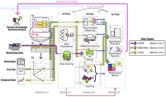
Figure 1.
The General, Explainable, and Verified Artificial Intelligence (GEVAI) Framework [1]. Multimedia, full-text, and temporal data can be considered as instances of Boolean data (BL), while multimodal data can be fit into Relational data (RL). Any domain knowledge coming from a Business Analyst can be encoded into an Upper Ontology expressible within Logic Programs (PL). The latter can also be updated once the analyst gains knowledge from the ex post phase, thus fine-tuning the system through human-in-the-loop intervention. Given the current limitations and open problems in orchestrating different Artificial Intelligence algorithms into a cohesive platform, we demonstrate how current attempts at designing AI pipelines align with our proposed scheme (FIDDP, EMeriTAte, and LaSSI).
2. Related Works
2.1. Verified AI
Verified AI aims to adopt verification mechanisms through correctness checking. Any Verified AI algorithm [2] relies on the notion of a system S, being the object of our study, and an environment E, in which such a system interacts. Specifications can either check whether S abides by it within the given environment (formal verification: ) or summarise system’s properties (specification mining). More formal characterization from the field [3,4,5] freely assume that specifications are explainable as they are expressible in logical form, as the definition of specifications lead to the generation of a system satisfying all the requirements given (formal synthesis). Notwithstanding this, the original survey does not constraint the representation for S, E, and to a specific formal language of choice, thus freely allowing more data-driven approaches. By walking under the assumption that human-like intelligence might be achieved by reasoning paraconsistently and given that the only known algorithms working as such are directly assuming a logical representation [6,7], this paper advocates that, ultimately, verified artificial intelligence should be expressed using a logical formalism. Given that it is always possible to extract a logical representation out of the data by “climbing the data-representation ladder” by further enriching raw data with additional contextual information, then it is always possible to reason paraconsistently over raw data after transforming it in a suitable formal representation. This will be remarked by the latest results from our work over hybrid explainability (Section 3.4.3 and Section 3.4.4). When considering a system varying in time through a set of snapshots [8,9,10], we can freely associate each snapshot to a different class or state , which can be compactly described through a specification . At this point, the agent simply observes the environment, and does not react to external stimuli: to achieve this, the agent has also to learn to associate an action to each state through a transition function , by which the system might potentially evolve through a reaction mechanism . We can then describe the co-evolution of an agent with it system with the following recurrence relationship [1] as discussed in continuous learning settings [11]:
2.2. Explainable AI
As the influence of AI expands exponentially, so does the necessity for systems to be transparent, understandable and, above all, explainable [12]. According to current literature [13,14], an AI algorithm is understood to be explainable when either the formal synthesis or specification mining algorithms return provide a specification that is intuitively understandable by the human. When this representation is perceived to be too distant from a suitable representation being immediately intelligible and appreciated by a human, we need to use other explainers correlating the input data to the predicted class.
On the other hand, this paper considers explainability in all the phases of an AI pipeline: we consider explaining the input data by injecting/enriching and cleaning data representations, the explicability of the inference process allowing us to derive the final reasoning task generating the desired specification, and the possibility of explaining the derived specification and possibly to determine its overall adequacy to fit the expected data. Considering the inference process at the centre of the artificial intelligence process and placing the input data and the results obtained respectively before and after the execution of this algorithm, we identify the phases previously defined as a priori (Section 3.1), ad hoc (Section 3.2), and ex post (Section 3.3). Within this categorization, explainable approaches can fit into two macro-categories, the static approaches (Section 3), considering only one possible kind of Explainable AI methodology where each algorithm might be considered as one single instantiation of a specific subcategory, and the hybrid ones (Section 3.4), considering a combination of multiple possible AI explanation technologies. Figure 1 summarises most of current literature on Explainable AI through the lens of a GEVAI framework (https://github.com/LogDS/GEVAI/releases/tag/v0.1, accessed on 29 May 2029).
As the extracted specifications mainly depend on the data representation of choice, and given that the former also forces a specific algorithm structure, we can achieve different level of algorithmic explanations by varying the data representation. This motivates a preliminary digression on the hierarchy of data representations (Section 2.2.1) before introducing the different types of explainability. Given that data can undergo transformations, thus including the inference process extracting rules as specifications from the data, we also need to consider provenance mechanisms to track the contribution of the original data inputs within the process of deriving the results (Section 2.2.2).
2.2.1. Data Representation Hierarchy
Talking about AI explainability requires first dealing with machine-level expressiveness by adding more contextual information to our data by increasing the amount of structure. Current literature recognises the current hierarchy of structured data representations [15]. As the choice of the final data representation of interest might be highly dependant on the choice of the ad hoc algorithm, the framework should be able to support a rewriting of any given representation into the desired format.
(Logic) Programs (LPs) provide a compact data representation also including logical connectives (S), thus including the notion of entailment when also describing rules (E), while supporting the definition of recursive predicates. We now discuss how we can represent the original complex data into less-structured forms, while loosing part of the inherent contextual information. By applying knowledge expansion algorithms (Section 3.1), we then obtain Relational (RL) data providing records from diverse relationships. It can adapt to both object-oriented and semistructured data models [16]. At this level, we completely lose any cognition of logical rules and connectives. By further degradation, we lose the information of distinct relationships, and we start focussing on just one relationship at a time: this is ultimately the Multi-Instance (MI) representation, we retain as in the former the relaxation of the First Normal Form (1NF) [17], which allows us the usage of nested content to express is-a or part-of hierarchical entailment [18]. Last, we can finitely break down each attribute-value association for each object at this level, thus including nested relationships, through Attribute-Value (AV) associations. It is often assumed that each AV record shall represent at most one fact, which shall also be associated with a probabilistic [19] or uncertainty [20] score. Given that values can only be either nominal (or categorical), ordinal (i.e., totally ordered), or continuous (in or any floating-point truncation), we completely lose any semantic information of nested relationships. Finally, we can further decompose the data by representing data entries as 0-ary atomic predicates [21] with associated truth values; for this reason, we refer to this representation as Boolean (BL). Atomic values can be simple data types and may include uncertainty scores through provenance information [22,23].
In logical frameworks that are as expressive or more so than First Order Logic (FOL), the inherent semi-decidability hampers the creation of converging inference algorithms. Consequently, data science tends to focus on restricted fragments of FOL, such as the alternating sequence of all universal quantifiers followed by existential quantifiers () [24], as well as Horn clauses prevalent in Prolog [25]. This approach allows algorithms to manage higher conceptual levels by treating programs as data, which aligns with the representation objectives in Verified AI domains.
2.2.2. Provenance
A data representation natively supports provenance information if each data record or object either provides a progressive and unique ID if coming from the original data source and provides an expression describing how it was obtained otherwise [23], thus allowing to directly derive the final uncertainty score associated to the resulting data rather than computing this continuously within the pipeline [19]. Provenance enables tracking of how the provided data was produced from the original data sources by taking into account the IDs referring to the original data while keeping track of the operations being applied to provide such results [26]. Provenance enables operational explainability among different phases of the pipeline [27].
2.3. General AI
General Artificial Intelligence has the pursuit of defining agents able to learn all the tasks as humans [28] while not being restrained by learning one single problem at a time (Artificial Narrow Intellignce). By doing so, each automated agent can be clearly be considered as a (human-like) mind [29]. Despite industrial [30] and academic [31] claims of Large Language Models (LLMs) providing early signs of GAI, there is strong evidence for this inadequately providing critical thinking capabilities. As a result of the autoregressive tasks generally adopted by generative LLM models, when the system is asked about concepts on which it was not trained initially, it tends to invent misleading information [32]. This is inherently due to the probabilistic reasoning embedded within the model [33], not accounting for inherent semantic contradiction implicitly resulting from the data through explicit rule-based approaches [34,35]. These models do not account for probabilistic reasoning by contradiction, with facts given as conjunctions of elements, leading to the inference of unlikely facts [36,37]. All these consequences are self-evident in current state-of-the-art reasoning mechanisms. They are currently referred to as hallucinations, which cannot be trusted to verify the inference outcome [38].
To address the former criticalities, this work works on some of the criticisms raised on the Penrose–Lucas argument by assuming one of the two possible alternatives: general intelligence can be achieved through an Turing Machine reasoning using some sort of paraconsistent logic [6,7] (Section 3.2). To achieve this, this work will support the need of pipelining different algorithms to actually achieve robust General AI providing logical representation of the data, while showcasing the limitations of loss minimisation driven algorithms, thus remarking on the limitations derivable from mainly using LLMs [32,33] for Artificial General Intelligence as presented in [31] over biased and contradictory data.
3. A Framework for General, Explainable, and Verified Artificial Intelligence (GEVAI)
This section extends the definitions originally provided in [1] by better reflection on the notion of explainability and categorizing all possible combinations and inter-operations of explainable algorithms. We say that an AI solution provides static explainability if only supports data (a priori, Section 3.1), specification extraction (ad hoc, Section 3.2), or result (ex post, Section 3.3) explanations. On the other hand, we say that an AI algorithm or pipeline provides hybrid explainability (Section 3.4) if it combines together several different types of explainability algorithms. In particular, we consider the following possible form of hybrid explainability: rip-cut, when the algorithm focusses of stacking together multiple different explainable algorithms of the same type (a priori, ad hoc, or ex post) [20], cross-cut, when the algorithm combines different explainability types together (e.g., a priori and ad hoc), and holistic, when any combination of the former is clearly provided. Table 1 summarizes the main type of artificial intelligence algorithms considered in the present paper: by expressing each algorithm of interest in terms of their type as in type theory, solidifies the claims of how to connect algorithms belonging to different phases as illustrated in Figure 1. After observing that each single algorithmic component can be expressed through a sub-instantiation of the GEVAI framework (Section 3.4.1), we also say that a data processing pipelin provides nested hybridation when one of its components is itself an instantiation of a hybridly explainable AI algorithm.

Table 1.
Representation of the input and output data types for all the algorithm considered by the present paper. denotes the subtype relationship, denotes an arbitrary explanation output, and denotes a finite function or record mapping data in X to Y. is used to denote the hyperparameters of interest under the assumption that the learning or mining algorithm will undergo specification search.
Given the impossibility of fully automating the entire approach due to many open problems addressed in our previous work [39], brought us to the decision to evaluate GEVAI from two different perspectives: first, we showcase the possibility of fully-automating current AI algorithms into a single pipeline under the assumption to deal with only AV data for classification tasks (Section 3.4.2); given the aforementioned open problem, we then instantiate GEVAI to perform two distinct classification tasks: multivariate time series classification (Section 3.4.3) and textual classification into entailment, indifference, and contradiction (Section 3.4.4). Section 4 provides an evaluation of these approaches, still under review.
3.1. A Priori
An a priori algorithm explains data by applying data transformations to it so to make it more accessible to the machine. Among these, we mainly distinguish between data cleaning and integration techniques, which mainly keep the data within the same representation and data hierarchy representation, from the ones climbing up the representation ladder, which are transforming less structured data into more structure data through the addition of contextual information. Within the latter case, any a priori explanation algorithm also providing a logical program describing the data is then considered a specification mining algorithm and, given that different ad hoc algorithms support different possible types of S data, enable the hybridation of multiple algorithms by gradually transforming the data. Ultimately, these techniques aim to use the machine itself to better explain the data to both the machine, further processing the data within the downstream process, and the human, which might provide data quality auditing within the loop. This process can be automated by designing an upper ontology serving as an E [40] for both data quality and reasoning purposes.
With respect to data cleaning algorithms, different data representation formats lead to different levels of data curation. When considering data in the AV format, data cleaning tasks fix values within single data fields according to rule-based or statistical data distributions [21,41,42,43,44]. When considering data in RL, we get more advanced data cleaning solutions which do not only replace single values in records, but also add or remove records so to fulfill data integrity constraint requirements [5,45]. When considering data in LP, we ultimately get data integration tasks aiming at uniforming different data representations with different schemas into one single global data representation [46,47], thus transforming records accordingly [48]. In all these scenarios, we can keep track of the uncertainty score reflecting the confidence of the transformation process [39]. Given that each data cleaning algorithm working at a higher data representation level will not tackle finer repairs and that no single data cleaning algorithm fully supports all the aforementioned type of repairs, provenance mechanisms act as an undoubtedly useful mechanism to reconcile data after cleaning has been occurring at different data abstraction levels. This motivates the adoption of an holistic framework for fulfilling all the aforementioned steps. Furthermore, we can also use the same data cleaning principles to actually generate new data from the initial system S [34,35,49,50] to derive inconsistent information. Thus, data cleaning algorithms mainly work as paraconsistent reasoning algorithms discussed in Section 3.2.4, thus generating a loop between ad hoc and a priori algorithms in Figure 1.
By climbing the data representation ladder up, we want to transform raw data, potentially represented in AV, into a higher level representation LP for enabling the usage of different data cleaning algorithms as well as applying more advanced ad hoc algorithms assuming different System representations (Section 3.2). With respect to Natural Language Processing tasks, common machine-learning algorithms do not only enable the transition from BL to MI through (multi-)word named entity recognition [51] aggregating distinct near words into one single entity while associating its type information (e.g., geographical location, geo-political entity, organisation, person), but also enable verb interpretation for extracting domain-dependant relationships, such as location_of and employee_of [52], providing greater human-level explicability. This also enables machine-level explainability, as text can be promptly digested into text to be inferred upon [53,54]. This approach is similar to image data analysis: while a preliminary step called object detection [55] aims to identify single parts of the image as entities, determining their relative position of in space and expressing this with explicit relationships [56] enables full RL data representation, which can be then easily represented in LPs as conjoined prepositions.
3.2. Ad Hoc
An algorithm provides ad hoc explainability if it motivates a specific decision leading to the generation of a specification. We say that such algorithm is marginally explainable if the suitability of the derived specification is compressed into a single numerical value, and we say that it is maximally explainable if each phase can be justified and logged with motivation. Such algorithms act as a black-box when there is a huge representation gap between the way the specification computes the result and the solution expected by a human, and is a white-box if its operation can be promptly translated in human language.
3.2.1. Classical Learning
Given an annotated dataset characterized as a (finite) mapping between data instances and corresponding classes in , the objective of a classical learning problem is to learn (and return) a single function referred to as a specification expressed in a target language while minimizing the classification errors across f [15]. usually varies with the learning problem of interest: while decision trees have as a set of all propositional formulas in disjunctive normal form over a finitary set of atoms bounded by the data values and the attributes occurring within the data, Deep Neural Networks will consider all th possible network configurations obtainable from one or more seed and neuron weight configurations. Thus, we can intend as the desired set of hyperparameters. This can be refined to fit the data through a loss function minimization problem [57]. Different learning algorithms might use different loss functions as well as their dual counterparts: while most statistical distributions exploit maximum likelihood estimation [58], decision trees [59] exploit impurity functions such as entropy measures or diversity indices [60].
Learning algorithms exploit hyperparameter tuning to avoid considering just one single local minimum [61], which is often considered as a time consuming process. More advanced approaches are starting pair the data space with the specification space: Extreme Learning Machines (ELMs) support an efficient weight initialization strategy through for hidden layers by exploiting training data values rather than being randomly assigned; this improves the running time to perform the learning task [62]. Similar approaches have been also been investigating in continuous learning: Broad Learning Structuress (BLSs) enables re-training of pre-trained model by adding augmenting the network structure with additional nodes which weights are also a function of the input training data. Notwithstanding the possibility of deriving a correlation between specification and data space, the process is still returning one possible hypothesis rather than multiple ones exhibiting similar desired characteristics.
The subsequent training process of both ELMs and BLSs will still undergo a loss minimization process: due to the minimisation problem not establishing an explicit explainable correlation between specification, quality measure (loss function), and data space, these methodologies cannot explain the rational of why a specific specification is to be preferred to other ones besides the reaching of a local minimum. Despite they can solve approximations of NP-complete problems [63], not providing an immediate understanding of the thought process while deriving the specification hampers the trustworthiness of the derivation process, which cannot be verified.
3.2.2. Mining
We now observe how the definition of an explicit ≼-generality notion across all specifications and the considering of a monotonic quality metric enables a more detailed explanation on why a given specification should be preferred to another in terms of data quality. When considering RL data, mining algorithms can also be used to derive integrity constraints from clean data [64]. When logical specifications are considered, this corresponds to the notion of entailment [65]. Mining algorithms achieve this [15] by structuring the specification search space as a lattice, where each node corresponds to a specification, while edges can be traversed from the most general towards the most specific through a refinement relationship . This is the preferred direction for efficiency purposes [65,66]. Differently from the learning algorithms, these guarantee the return of multiple possible specifications adhering to a specification space rather than returning just one single specification. The structure of the specification search clearly skews the search to prefer overly-represented data to less frequent one, thus implicitly assuming that the data is cleaned and unbiased. On the other hand, this cannot be generally assumed for real data, where biased content is relatively abundant as it is known to travel faster than reliable information [67], thus dominating in size over trustworthy data.
3.2.3. Relational Learning
The relational learning algorithms restrict the specification language, the System, and Environment to be in LP, usually in the domain of Horn clauses. This is achieved by supporting learning through many different relationships while potentially decomposing data relationships according to functional dependencies in E for then learning rules that are independent from a specific database schema [68]. These approaches improve over the criticisms raised by both of the former approaches, as they can both generate multiple possible specifications as per mining algorithms, while also providing safer learning conditions as they neither require statistically independent and uniformly distributed examples, while also allowing to learn from inconsistent databases being violations to the criteria from E [42]. These algorithms, differently from mining ones, prefer specific-to-general data traversals to ensure good generality properties [42]. Differently from the other two approaches, these algorithms also require the usage of the Environment (e.g., TBox) to strengthen the quality of the data-derived specification. Despite the possibility of using the information from E to derive contradiction, this cannot still completely address real data at its fullest. To prevent the generation of inconsistent hypothesis formulations from the data, these algorithms are focusing on clauses with neither negations nor the universal falsehood as their heads. This implies that every instance of the LP data or S eliminates logical connectors. Consequently, these methods are unable to identify data inconsistencies, even when considering hierarchical data information. Moreover, the same stringent assumption regarding rule formulation restricts the applicability of the learning algorithms, as they cannot be utilized in other, more realistic situations that require comprehensive data transformation operations. Last, these approaches are still relying on explicit data annotations remarking which data samples are positive or negative data, which cannot be always determined from real-world crawled data [69].
3.2.4. Paraconsistent Reasoning
Probabilistic reasoning cannot be trusted for detecting and reasoning over conflicting and contradictory information within the data [36] as “rational acceptance based on a probability threshold cannot be closed under logical consequence” and, most importantly, “it will not be closed under conjunction” as this might derive into the generation of unlikely consequences [37]. This then motivates using paraconsistent reasoningby reasoning in a purely logical way by first ignoring the uncertainty scores, to then use later on within a subset of consistent information. These also overcome limitations from Relational Learning algorithms by not assuming data to be labelled, and by considering data to be fully represented in LP, thus including logical connectors such as negation. Under these conditions, most of the Machine Learning (ML) algorithms will fail, for which it is then important to determine the number of contradictions in S by merely relying on an environment E assumed to contain trustworthy and correct information [69]. This will then require us to pose a greater control to the overall inference mechanism, thus increasing the explainability of the overall inference process to also ponder over conflicting data representations. One possible way to do so is to block trivialization of the reasoning through disjunction-free LPs where rules’ head have no disjunctions, tails can also express weak negation, and where the universal falsehood can only appear within the heads. This process is guaranteed to converge as determining the consistency of such programs is in NP [70]. By only using logical-driven derivations for determining relevant feature informations, this approach is trivially non-biased by data distributions and frequency.
To the best of our knowledge, none of the existing algorithms for paraconsistent reasoning is actually used to derive specifications as per Relational Algorithms, but specifications can be understood as either the sets of Maximally Consistent Specifications (MCS) [71] or deriving Minimal Inconsistent Sets (MIS) through the expansion phase [72]. The latter is the only one being actually implemented for dealing with real world data solutions by making inference mechanisms using the Closed-World Assumption (https://github.com/jackbergus/java_logicalconsistency, accessed on 30 May 2025) [35]. As a consequence of the former, these algorithms are mainly understood as ways to clean the data and find incongruences when expressed in the same language of the specifications, rather than extracting summarized data descriptions as specifications themselves. Future works should address the possibility of hybridize paraconsistent reasoning with relational learning solutions, so to ultimately learn to extract rules while considering as many data classes as coherently set of similar data elements.
3.3. Ex Post
We consider ex post explainability as the ability to characterize a specification, possibly derived from a ad hoc phase by transforming it into a different representation, which can be potentially mediated by the system or environment information. This is marginally explainable if the specification is just compressed into a score, and maximally explainable if the correlation between the data and the expected classification is also encompassing correlations within the data instances. The forthcoming subsections will introduce distinct approaches in order of increasing explainability.
3.3.1. Performance Metrics
Performance metrics used for both classification or mining tasks are interoperable, in the sense that they provide a single numerical value representing the discrepancy from the testing data and the values predicted from it. On the other hand, the resulting explanation cannot be used within other subsequent AI tasks, and so it provides minor interoperability which is mainly related to fine-tuning. As each metric is also well-ground and defined in literature, they are easily interpretable by a human, despite providing none to little information to the motivations leading to the potential classification outcome.
3.3.2. Specification Agnostic
Specification-agnostic explainers [14] extract correlations between input data and expected classification outcome, where correlations across input data is limited. Thus, they place themselves halfway through performance metrics and simple specification extractors. As such explainers require additional re-training, they often act as an ad-hoc algorithm paired with some immediately understandable graphical representation of the final classification outcome. While LIME [73,74] returns a linear specification tangent to the predicted data points, SHAP [75,76] assign a value to each feature similarly to a logistic regression specification, thus providing confidence score predictions for each of the arguments. Their adaptability to support explanations for disparate data representations such as images [73] or full-text [74] enhances their interpretability. When considered as ad hoc algorithms, their performance cannot be promptly tested using the aforementioned metrics directly, while requiring some additional specification post-processing [77].
3.3.3. Extractors
Ex Post explainers can be also operate as extractors, simply rewriting the specification from a data driven into a mathematical representation. In particular, this phase mainly trasforms the specification from a description easily digestible for a machine, into a notation which is understandable by a human. Then, the explainability of the extracted specification will be highly dependant on the white- or black-box nature of the ad-hoce phase itself. When considering the interpretation of dense layers under the assumption that each neuron within the same layer will be associated with the same activation function [78], we can then obtain the following algebraic formulation of a feed-forward network:
On the other hand, the extraction of a specification from a specification from a white-box model such as a decision tree generates one propositional formula in disjunctive-normal-form for each class occurring within the training dataset. In both circumstances, the interpretability of the result is highly dependant on the distance between the final specification language and a notation more easily digestible by a human. This should also include the compactness of the specification being originally derived. Notwithstanding the former, these solutions are maximally explainable, as they provide clear correlation not only between data input and output, but also remark how correlations across data inputs lead to the classification outcome.
3.4. Hybrid Explainability
3.4.1. Financial Institution DeDuplication Pipeline (FIDDP)
This section showcases the generality of the framework by remarking how previous data processing pipelines can fit the aforementioned framework. In particular, we consider the FIDDP [20] as a specific instance of the baseline data deduplication pipeline (BLDDP), both working over AV data. As this pipeline provides data cleaning capabilities, FIDDP acts as an a priori algorithm. Notwithstanding this, each of its phases can be mapped within the GEVAI framework, thus providing an instance of an holistic hybrid explainability pipleine, as it composes both a priori and ad hoc algorithms. FIDDP considers two main a priori algorithms for preliminary data pre-processing and a final ad hoc clustering algorithm; while the former first determines the region of records that might be potential duplicates for then “blocking” the most similar ones into one region through pairwise record similarity, the latter uses the pairwise record similarity computation to cluster similar records, thus coalescing all the ones likely to refer to the same physical person. As these phases are also used to pick the best hyperparameters and algorithms for the subsequent tasks, each task works as a fine tuning mechanism (Figure 1) for the following phases through an implicit ex post phase.
3.4.2. Automating AI Benchmarking with AV-GEVAI
This section considers a specific preliminary implementation of the GEVAI framework, AV-GEVAI, showcasing how GEVAI can be also used as a benchmarking tool for testing multiple machine learning (ad hoc) and explainers (ex post) while also considering their performance in terms of both running time and classification scores (ex post) by assuming data being expressed in AV, thus in tabular or matrix format. In this scenario, the data cleaning strategy is minimal and highly dependant on the specificity of the ad hoc algorithm receiving the data: if the algorithm supports only numerical data (e.g., DecisionTree implementation from scikit-learn [79]), then we exploit one hot encores to map categorical data into their numerical counterpart. When multiple other representations are preferred, it is a common practice on AI pipelines to provide multiple possible data transformation solutions, to then decide which of these is the best fit for the specific task of interest [80]. Furthremore, given that most algorithms do not need explicit attribute information, this is discarded in the a priori phase, but still retained for further processing.
Within each algorithm of the ad hoc phase, we also perform hyperparameter tuning to return the best model configuration leading to the best prediction outcome. To remark the possibility of integrating together disparate types of learning algorithms, this paper considers the following solutions: Decision Trees [81], which construct a hierarchical, tree-like structure to map features to outcomes, RipperK [82], a rule-based algorithm that generates a concise set of if-then rules by iteratively growing and pruning conditions to cover training instances, and Neural Networks with Network Architecture Search [83] which employs a automated search strategy to determine an optimal Neural Network (NN) architecture, rather than relying on a manually predefined structure. While the first two are examples of white-box classifiers, the last one is an example of a black-box one. At this stage, we also perform additional data transformation if required by the algorithm: As RipperK was designed to solve a binary classification problem and not a multi-class one, we further pre-process the dataset to transform it into a binary problem so to solve the one-vs.-rest problem [84], through which we train as many classifiers as the number of classes within the dataset, while requiring the algorithm to recognize one class against the rest; we then use the following ensemble method for determining the predicted class out of each singularly trained classifier: we return the class which was predicted with the highest confidence. We then consider all types of ex post algorithms with for mainly benchmarking the solutions; a similar approach is also considered in EMeriTAte(+DF) (Section 3.4.3), where the ex post phase is mainly used to test the specification resulting from the multivariate time series classification problem. LaSSI (Section 3.4.4), on the other hand, subverts the categorization provided by Section 3.3, for which the derivation of an explanation of the classification outcome requires an inference process for producing a single result, which can be represented as both a specification and a single numerical value.
3.4.3. (DataFul)Explainable Multivariate Correlational Temporal Artificial Intelligence (EMeriTAte+DF)
EMeriTAte+DF [9] is a hybrid explainability pipeline for multivariate time-series classification with holistic features, where time series classifications’ explanation comes from a white-box decision tree classifier enabling the correlation of the different trends occurring within the numerical data discretized and summarized in a preliminary ad hoc phase. This work was originally designed for characterising dyskinetic events in Parkinsonian patients, where each dimension might refer to a different motor sensor and estimated blood concentration level of a specific active principle given a pointwise drug assumption pattern. While doing this, the clinician must gain medical insight from the MTS classification, thus requiring an explainable and declarative representation of the motivations leading to the dyskinetic event.
The correlation between numerical trends occurring across dimensions is enabled by a preliminary climb of the representation ladder, where for each time series dimension the a priori phase extracts data trends (DT) [85] describing arbitrary increase, decrease, or volatility patterns while considering them with different lengths. These discretised data trends are then transformed into durative events where, differently from both the previous work [8,85] itself, each durative event was extended to support summarized statistics (Catch22 [86]) concerning the specific dimension to which the durative event refers to. Such event information is then collected into a log: in a second a priori step, such log is transformed into as many logs as the classes present across all MTSs, where each trace will represent a maximal contiguous set of events always associated with the same classification label. Next, two ad hoc phases first mine temporal clauses with data predicate using a dataful extension of Bolt2 [65], where clauses co-occurring in different time series classes are extended with data features considering values from Catch22 statistics. Then, the extracted temporal clauses are assembled through a white-box classifier (DecisionTrees) describing each temporal class with a set of temporal behaviour occurring. Last, an ex post extractor returns the learned decision tree providing a temporal explanation of the different possible behaviours distinguishing different temporal classes.
3.4.4. Logical, Structural, and Semantic Text Interpretation (LaSSI)
LaSSI [53,54] provides for the first time a fully-explainable pipeline for full-text interpretation. This research paper introduces a novel cross-cut hybrid explainability pipeline that combines graphs and logic to generate First-Order Logic (FOL) representations, accurately capturing full-text similarity. The paper aims to address issues with current Machine Learning (ML) techniques and classifiers trained on generative language models, which struggle to differentiate between logical implication, indifference, and inconsistency for text classification tasks. The ad hoc phase extracts the logical representation from the given full text; graphs are generated as intermediate representations from dependency parsing [87]. Dependency graphs are then rewritten to uniform the syntax (active/passive voice) to a similar reprsentation according to the grammatical rules of the language [16]. When sentences with equivalent meaning produce structurally disparate graphs, equality formulae are obtained. Overall sentence similarity is then derived by reconciling such formulae with minimal propositions. This phase exploits contextual information as retrived through the a priori phase to facilitate the preliminary identification of entities within the text: not only authors extract and identify multi-word entities by cross-comparing terms occurring from online word nets, but also associate specific type information to each entity occurring in the text. For example, authors also extract temporal (SUTime [88]) and spatial (GeoNames [89]) information: this distinction is then retained to differentiate between the disparate logical functions of propositions occurring within the text. This phase appears to be crucial, as missing this early identification phase leads to a degradation in classification performance by lacking the necessary context and relational information to interpret the text semantically. The final logical representation returned by the ad hoc phase employs a straightforward extension of First-Order Logic (FOL), whereby entities can be associated to modalities (some, all). Last, the ex post phase proposes a novel specification agnostic explainer for LP data: it takes the sentences as rewritten in the ad hoc phase and utilizes logical rewriting techniques to finally produce a confidence score embedding whether the two sentence are implying, indifferent, or contradictory. Thus, the confidence score provides a sentence similarity score capturing the possible world where the two sentences, when represented logically, hold. This achieves simplistic paraconsistent reasoning by removing all the worlds where different atoms cannot jointly hold. The pipeline carries out reasoning through a preliminary Upper Ontology and some logical rules for deriving the similarity of the atoms occurring within each formula. Thus, the proposed ex post phase exploits an ad hoc reasoning
4. Evaluation
4.1. AV-GEVAI
The evaluation tests different learning algorithms embedded in GEVAI over the wine preferences dataset [90] providing both numerical and categorical data, and use this to train both decision trees as a representative of white-box learning algorithms [91], deep neural networks with network architecture search as a representative of black-box learning algorithms [83], and RipperK as a representative of white-box relational learning algorithms [82]. We consider both LIME and SHAP as model agnostic explainers, while considering accuracy, F1, Precision, and Recall as performance metrics. We consider micro averaging, for an easily understandable metric for overall model performance regardless of class, and macro averaging, to treat all classes equally. Despite this paper choosing some of the results produced by this pipeline, the online repository disclose the full set of the results produced by the pipeline (https://osf.io/6jf5z/?view_only=112ebdd0156444ddbb8cf6ea53729949, accessed on 30 May 2025).
4.1.1. Efficiency
For classical learning tasks, RipperK’s training process (Generating model) is the most time-consuming, as shown in Figure 2 (except for the white box explanation). This arises from its logical-driven methodology, which involves an initial rule-growing stage, followed by iterative pruning of rules using a separate pruning set, and finally, an optimisation phase for the entire rule set to enhance accuracy and reduce complexity, a thorough approach that, while fostering robust rule generation, is computationally intensive. This is also motivated by the adoption of a brute-force approach for generating the rules and navigating the data space, which does not reflect the same structure from other relational learning algorithms, while also requiring to re-run the algorithm for each class appearing within the dataset. On the other hand, Decision trees provide the most efficient solution, as they use an effective greedy impurity-based heuristic to derive predicates, while testing predicates over lesser and lesser data samples.
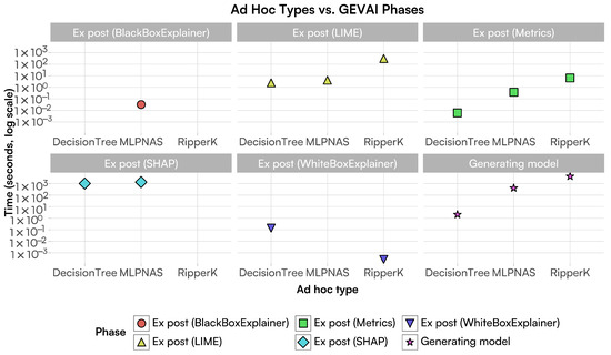
Figure 2.
Comparison of different phases of the GEVAI framework, showing how long training time takes for collecting the ad hoc models, as well as five different ex post phases.
The derivation of LIME explanations is globally more efficient than extracting SHAP ones. The reason has to be sought in the different implementation of the two solutions. For a given instance to be explained, LIME generates a new dataset of perturbed samples in the vicinity of that instance, then obtains predictions for these perturbed samples from the original model. Finally, LIME trains an interpretable model on this dataset, where samples are weighted by their proximity to the instance of interest, where the explanation is derived (https://christophm.github.io/interpretable-ml-book/lime.html, accessed on 30 May 2025). On the other hand, the calculation of Shapley values for SHAP is computationally demanding, requiring the evaluation of the model’s output for all possible subsets of features, known as coalitions. For a model with p features, there are such subsets, consequently making the computation time exponential (https://christophm.github.io/interpretable-ml-book/shapley.html, accessed on 30 May 2025). This motivates why using a SHAP explainer produces the longest training times out of all the ex post methods, with RipperK meeting our computation timeout, still not producing a result after two days, thus never succeeding in producing an explanation in a reasonable time frame.
4.1.2. Explainability
The following compares and explains the different ex post phases, where examples for just Decision Trees are given, as it was the second best performing model according to the Performance Metrics in Table 2. These results aim to show that all these approaches provide orthogonal observations describing trained specifications under different perspectives, thus motivating their simultaneous adoption within a solution benchmarking pipeline.
Table 2.
Classification metrics for different ad hoc pipelines within GEVAI framework. Numbers in blue and red highlight the best and worst scores respectively per metric type and average.
Performance Metrics
We now discuss the results coming from the classification performance metrics applied to all the ad hoc algorithms of interest, and reported in Table 2.
Despite RipperK typically producing the largest running times for explanations, it performs the best for at least one average for each metric type. This could be attributed to RipperK constructing rules by iteratively adding conditions to cover positive examples of a class while excluding negative ones. A crucial aspect is its pruning mechanism, which simplifies rules based on their performance on a validation set, which helps to avoid overfitting to the training data and improve generalisation on unseen instances. MLPNAS performs the worst in all metrics, this may be caused by over or underfitting by being too complex or simplistic for the given dataset, a common problem when training NNs as modification of many hyperparameters can be difficult to optimise. This then postulates that logical based approaches, despite being generally slower to train due to simplistic algorithmic implementations, usually provide better accuracy results by using explainable and traceable motivations on why specific specification might be refined or discarded.
Extractors
Black-box extractors for MPLNAS were very hard to interpret, as the provision of several different equations interconnected with each input dimension generated a substantially huge file, which was hardly interpretable. This mainly motivates the adoption of specification agnostic ex post algorithms for NN solutions.
Given that white-box extractors either rewrite the generated model into a high level representation (Decision Tree) or are directly provided in the suitable logical representation (RipperK), these type of explanations are quite efficient to extract, without any further data processing or learning tasks.
The output in Figure 3a describes four distinct decision rules from a Decision Tree model, each outlining a specific path to a classification. Each rule consists of one or more conditions on input features, such as feature_11 <= 10.11667, where data is split based on whether a feature’s value meets a certain threshold. The and operator signifies that all conditions within a rule must be met. The => Label=X part indicates the predicted class if an instance satisfies all the rule’s conditions. Finally, the (0/0) at the end of each rule represents (misclassified instances / total instances) for that specific path, suggesting that these particular rules perfectly classified all training instances they covered. For instance, the first rule means if feature_11 is less than or equal to 10.11667 and feature_2 is less than or equal to 0.23750, the model predicts Label=2 with no misclassifications for the data fitting this rule. A more graphical visualisation of this can be seen in Figure 3b.
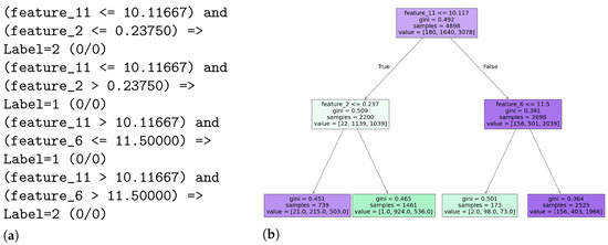
Figure 3.
Side-by-side comparison of Decision Tree rule explanations and visualisation for the same rules: (a) a textual representation versus (b) a tree visualisation.
Specification Agnostic
While performance metrics mainly focus on the adequacy of the specification to describe the system and extractors mainly are an explicable way to derive the motivation that the specification generates to derive the classification outcome, specification agnostic classifiers mainly focus on the significance of each feature to influence the final classification outcome. This feature importance is also conveniently plot into easily interpretable representations.
LIME plots (Figure 4) display bar charts where each bar corresponds to a feature. The length of the bar illustrates the feature’s importance for that particular prediction. By examining the features with the longest bars, we can easily understand which factors were most influential in the model’s decision for that instance.
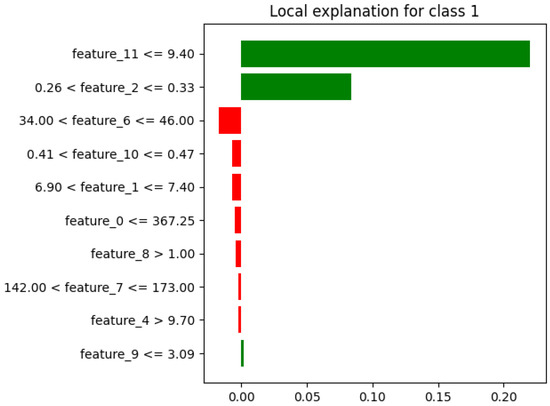
Figure 4.
Example LIME plot output for class 1 for a Decision Tree model.
SHAP plots show which features most influenced the model’s prediction for a single observation: features coloured in red increase the confidence of the prediction, while ones in blue lower the estimation. These values are laid along a horizontal axis while meeting along the line reflecting the classification outcome. This allows us to identify the most significant features and observe how their varying values correlate with the model’s output.
Figure 5 shows a summary SHAP plot, providing a global overview of how each feature impacts a given Decision Tree’s predictions across many instances. Features are ranked vertically by their overall importance, with the most influential feature at the top. A distribution of its Shapley values are displayed for every instance in the dataset, where the horizontal position of each point indicates the SHAP value for that instance, showing whether the feature pushed the prediction higher or lower compared to the baseline. Furthermore, these points are often coloured based on the actual value of the feature for that instance (red for high values, blue for low values), so values can be visualised to show positive or negative impact on the prediction.
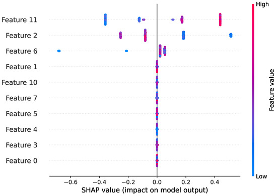
Figure 5.
Example Summary SHAP plot for a Decision Tree model’s output.
4.2. (DataFul) Explainable Multivariate Correlational Temporal Artificial Intelligence (EMeriTAte)
These experiments remark on the possibility of using a fully-fledged logical-based approach to learn from numerical data. This paper presents a subset of the results discussed in [9], to which we refer the reader for more in-depth analysis. Such results suggest that competing state-of-the-art approaches, thus including ones considering Deep Neural Networks (DNNs) with attention mechanisms, fail to correctly classify the resulting events due to their impossibility of explicitly deriving explicative correlations across different dimensions for complex multidimensional patient data. This proves that achieving a better human-driven explanation can also help the machine to draw better machine specifications.
Figure 6 remarks that the proposed methodology exhibits similar behaviour if compared to other state-of-the-art approaches when considering simpler datasets, while significantly outperforming them over novel datasets with a considerable number of dimensions and exhibiting complex interactions across different numerical dimensions. This remarks that, as far as the current datasets are concerned, the proposed methodology is not only able to not lose relevant information for the classification task, but it is also able to extract further information deemed relevant to address classification tasks in more challenging datasets.
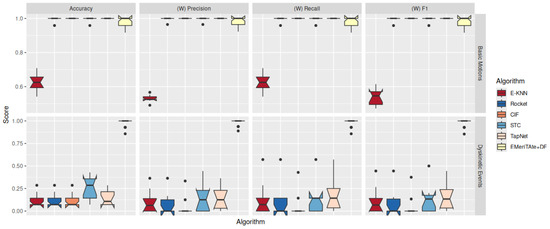
Figure 6.
Classification Performance Metrics for two mobility datasets, one for basic mobility (Basic Motions, multi-class classification) and the other for Diskinetic events (binary classification) in Parkinson Disease patients. We provide weighted scores for multi-class classifications [9].
Figure 7 shows that the price that needs to be paid to obtain this improvement on performance is an increase of computational cost for training the algorithm, mainly hampered by establishing all the correlations occurring within the data across different time series dimensions. EMeriTAte+DF is even more affected by this due to an additional clause refinement process leveraging data features associated with the DT patterns and considered within the Declare clauses composing the final propositional model. For smaller datasets exhibiting lesser interactions, its training time is still comparable with neural-network based approaches (TapNet) which are not providing explanations for the classification outcome.
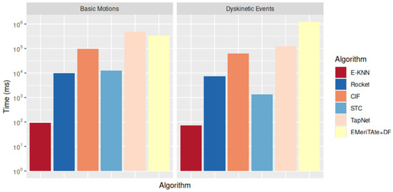
Figure 7.
Running times from two datasets for multivariate time series classifications (Basic Motions and Diskinetic Events) [9].
4.3. Logical, Structural, and Semantic Text Interpretation (LaSSI)
As LaSSI also enables the comparison between LaSSI and other pre-trained model for carrying out a sentence classification task, this pipeline also achieves holistic explainability, as it also enables the usage of specification-agnostic explainers over the results derived from other methodologies and to compare with the results provided by LaSSI.
The latest results from the authors [54] remark that, despite LIME and SHAP might provide explanations for both classical text and pre-trained text classifier that might be easier to read, the resulting explanations might be wrong for two distinct and opposite reasons: either the traditional sentence classifier provides correct predictions but targets wrong explanations why sentences should entail each other (Figure 8a,c), or the classifier itself provides the wrong prediction, thus nullifying the meaningfulness of the final explanation (Figure 8b,d). When asked to return to derive sentence similarity for information present within the Upper Ontology, LaSSI provides correct explanations which are not only considering single words occurring within the full text, but whole atoms referring to specific, as it does not rely on a third party explainer to derive the explanations, rather than actually explaining the internal inference process leading to the provided result (Figure 9).
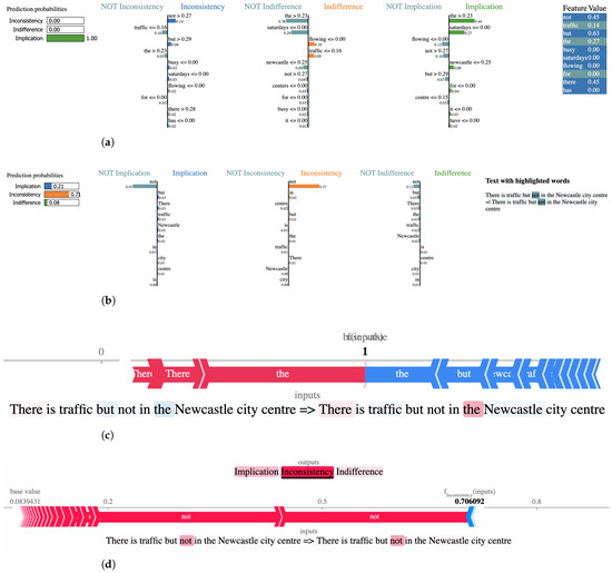
Figure 8.
LIME and SHAP explanations comparing “There is traffic but not in the Newcastle city centre” against itself [54]. (a) LIME explanation using TF-IDFVec+DT, highlighting the word “the” in both NOT Indifference and Implication, leading to a 100% confidence for an Implication classification. (b) LIME explanation using DistilBERT+Train, highlighting the word “not” leading to a NOT implication and Inconsistency classifications, ultimately resulting in an Inconsistency classification. (c) SHAP explanation using TF-IDFVec+DT, highlighting the model’s confidence in the word “the” leading to a Implication classification (1 for the image above). (d) SHAP explanation using DistilBERT+Train, highlighting the model’s confidence in the word “not” leading to an Inconsistency classification.
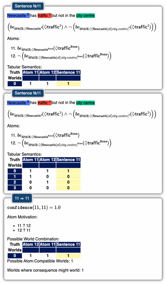
Figure 9.
LaSSI explanation shows 100% implication between the same sentence from Figure 8. Highlighted parts refers to entities captured in the a priori phase, the logical formulae refer to the final result of the ad hoc phase, while the computation of the confidence score refers to the computation from the ex post phase [54].
Additional experiments evaluating the pipeline’s capabilities in understanding and processing sentences that involve spatiotemporal nuances also remarked the shortcomings of state-of-the-art pre-trained models. The experiments considered sentence transformers for deriving sentence similarity scores (T1 and T2: All-MiniLM-L6/12-v2 [92], T3: All-mpnet-base-v2 [93], T4: All-roberta-large-v1 [94]), GPT-based classifiers distinguishing between entailment and indifference in text (T5: DeBERTaV2+AMR-LDA [95]), and neural information retrieval approaches (ColBERTv2+RAGatouille [96]). None of the former approaches were also been used to explicitly target inconsistency or conflicting information. Hybrid explainability helps the machine to derive correct results by mimicking similar logical-based reasoning that are common in humans, while the machine-driven numerical approximation cannot correctly grasp for the textual nuances by not deriving explanations for entire passages, while focussing on single word compositions with no explicit correlation provided as an input (see Table 3).
Table 3.
Classification Performance Metrics for spatiotemporal sentences, with the best value for each row highlighted in bold, blue text and the worst values highlighted in red. The classes are distributed as such: Implication: 32, Inconsistency: 27, Indifference: 110. Numbers in blue and red highlight the best and worst scores respectively per metric type, average, and clustering metric for deriving the classes’ cut off.
5. Discussion and Future Works
This work provides preliminary results showcasing the benefits of exploiting verified artificial intelligence to achieve human-level explanations that not only correlate input features with classification outcomes, but also establishes correlations across features. By comparing different AI solutions and by reflecting on the criticisms on the Penrose-Lucas argument, we also outline how paraconsistent reasoning should be used to reason over data within complex scenarios which, when backed up with a full-fledged Upper Ontology, outperform state-of-the-art artificial intelligence solutions. Preliminary results over the AV fragment of data representations show the possibility of automating data analysis pipelienes to solve simple tasks, while remarking the possibility of using the same framework not only to solve machine learning problems, but also to benchmark already existing solutions.
Notwithstanding the former, the codebase only provides these pieces singularly, with no current automation for orchestrating these pieces. This is also a common problem with other data science approaches [97], as they require the user to connect the components manually. Similar considerations can be made for AI pipelines, which still require a huge amount of manual intervention. Fully automating this framework to achieve AGI require to solve open problems from current literature, which are also related to the problem of orchestrating multiple agents [39]: first, current machine learning pipelines do not fully support the integration of disparate data sources into a cleaned and cohesive framework as relationship are mainly merged into one single universal relationship [98], despite the foundational basis on data integration and data cleaning also considering data information evolving through time [47]. Furthermore, some data processing tasks still require human-in-the-loop assistance [99]. By pairing this contextual and semantic data information with the type properties associated with each algorithm (Table 1) and after expressing the user information needs as goals to be achieved by a task, we can then straightfowardly exploit planning algorithms [100] to orchestrate the combination of different pipeline tasks to orchestrate different algorithms. Such orchestration can be dynamically updated to reflect sudden changes to the user needs or to adapt to different environmental set-ups [101]. Future works will address the theoretical possibility of defining this orchestration by including both planners and data integration features as major components of the GEVAI framework.
Author Contributions
Conceptualisation, G.B.; methodology, G.B.; software, G.B. and O.R.F.; validation, G.B.; formal analysis, G.B.; investigation, G.B.; resources, G.B.; data curation, G.B. and O.R.F.; writing—original draft preparation, G.B.; writing—review and editing, G.B. and O.R.F.; visualisation, O.R.F.; supervision, G.B.; project administration, G.B.; funding acquisition, G.B. All authors have read and agreed to the published version of the manuscript.
Funding
This research received no external funding.
Institutional Review Board Statement
Not applicable.
Informed Consent Statement
Not applicable.
Data Availability Statement
The preliminary release of the GEVAI project is available at: https://github.com/LogDS/GEVAI (accessed on 28 July 2025). Result data can be found at: https://osf.io/6jf5z/?view_only=112ebdd0156444ddbb8cf6ea53729949 (accessed on 28 July 2025).
Conflicts of Interest
The authors declare no conflicts of interest.
References
- Bergami, G.; Fox, O.R.; Morgan, G. Extracting Specifications Through Verified and Explainable AI: Interpretability, Interoperability, and Trade-Offs. In Explainable Artificial Intelligence for Trustworthy Decisions in Smart Applications; Springer: Cham, Switzerland, 2025; Chapter 2; in press. [Google Scholar]
- Seshia, S.A.; Sadigh, D.; Sastry, S.S. Toward verified artificial intelligence. Commun. AC2 2022, 65, 46–55. [Google Scholar] [CrossRef]
- van der Aalst, W.M.P. Process Mining-Data Science in Action, Second Edition; Springer: Berlin/Heidelberg, Germany, 2016. [Google Scholar]
- Bergami, G.; Maggi, F.M.; Montali, M.; Peñaloza, R. A Tool for Computing Probabilistic Trace Alignments. In Proceedings of the Intelligent Information Systems-CAiSE Forum 2021, Melbourne, VIC, Australia, 28 June–2 July 2021; Nurcan, S., Korthaus, A., Eds.; Lecture Notes in Business Information Processing; Springer: Berlin/Heidelberg, Germany, 2021; Volume 424, pp. 118–126. [Google Scholar]
- Bergami, G.; Maggi, F.M.; Marrella, A.; Montali, M. Aligning Data-Aware Declarative Process Models and Event Logs. In Business Process Management; Polyvyanyy, A., Wynn, M.T., Van Looy, A., Reichert, M., Eds.; Springer: Cham, Switzerland, 2021; pp. 235–251. [Google Scholar]
- Megill, J.L. Are we paraconsistent? On the Luca-Penrose argument and the computational theory of mind. Auslegung J. Philos. 2019, 27, 23–30. [Google Scholar] [CrossRef]
- LaForte, G.; Hayes, P.J.; Ford, K.M. Why Gödel’s theorem cannot refute computationalism. Artif. Intell. 1998, 104, 265–286. [Google Scholar] [CrossRef]
- Bergami, G.; Packer, E.; Scott, K.; Del Din, S. Predicting Dyskinetic Events Through Verified Multivariate Time Series Classification. In Database Engineered Applications; Chbeir, R., Ilarri, S., Manolopoulos, Y., Revesz, P.Z., Bernardino, J., Leung, C.K., Eds.; Springer: Cham, Switzerland, 2025; pp. 49–62. [Google Scholar]
- Bergami, G.; Packer, E.; Scott, K.; Del Din, S. Towards Explainable Sequential Learning. arXiv 2025, arXiv:2505.23624. [Google Scholar]
- Camacho, A.; Toro Icarte, R.; Klassen, T.Q.; Valenzano, R.; McIlraith, S.A. LTL and Beyond: Formal Languages for Reward Function Specification in Reinforcement Learning. In Proceedings of the Twenty-Eighth International Joint Conference on Artificial Intelligence, IJCAI-19, Macao, China, 10–16 August 2019; Volume 7, pp. 6065–6073. [Google Scholar]
- Maltoni, D.; Lomonaco, V. Continuous learning in single-incremental-task scenarios. Neural Netw. 2019, 116, 56–73. [Google Scholar] [CrossRef] [PubMed]
- Tammet, T.; Järv, P.; Verrev, M.; Draheim, D. An Experimental Pipeline for Automated Reasoning in Natural Language (Short Paper). In Automated Deduction–CADE 29; Pientka, B., Tinelli, C., Eds.; Springer: Cham, Switzerland, 2023; pp. 509–521. [Google Scholar]
- Zini, J.E.; Awad, M. On the Explainability of Natural Language Processing Deep Models. ACM Comput. Surv. 2023, 55, 103:1–103:31. [Google Scholar] [CrossRef]
- Dwivedi, R.; Dave, D.; Naik, H.; Singhal, S.; Omer, R.; Patel, P.; Qian, B.; Wen, Z.; Shah, T.; Morgan, G.; et al. Explainable AI (XAI): Core Ideas, Techniques, and Solutions. ACM Comput. Surv. 2023, 55, 1–33. [Google Scholar] [CrossRef]
- de Raedt, L. Logical and Relational Learning: From ILP to MRDM (Cognitive Technologies); Springer: Berlin/Heidelberg, Germany, 2008. [Google Scholar]
- Bergami, G.; Fox, O.R.; Morgan, G. Matching and Rewriting Rules in Object-Oriented Databases. Mathematics 2024, 12, 2677. [Google Scholar] [CrossRef]
- Elmasri, R.A.; Navathe, S.B. Fundamentals of Database Systems, 7th ed.; Pearson: London, UK, 2016. [Google Scholar]
- Johnson, J. Hypernetworks in the Science of Complex Systems; Imperial College Press: London, UK, 2011. [Google Scholar]
- Fuhr, N.; Rölleke, T. A Probabilistic Relational Algebra for the Integration of Information Retrieval and Database Systems. ACM Trans. Inf. Syst. 1997, 15, 32–66. [Google Scholar] [CrossRef]
- Andrzejewski, W.; Bębel, B.; Boiński, P.; Wrembel, R. On tuning parameters guiding similarity computations in a data deduplication pipeline for customers records: Experience from a R&D project. Inf. Syst. 2024, 121, 102323. [Google Scholar]
- Rekatsinas, T.; Chu, X.; Ilyas, I.F.; Ré, C. HoloClean: Holistic Data Repairs with Probabilistic Inference. Proc. VLDB Endow. 2017, 10, 1190–1201. [Google Scholar] [CrossRef]
- D’Agostino, G.; Reed, C.A.; Puccinelli, D. Segmentation of Complex Question Turns for Argument Mining: A Corpus-based Study in the Financial Domain. In Proceedings of the 2024 Joint International Conference on Computational Linguistics, Language Resources and Evaluation, LREC/COLING 2024, Torino, Italy, 20–25 May 2024; pp. 14524–14530. [Google Scholar]
- Green, T.J.; Karvounarakis, G.; Tannen, V. Provenance semirings. In Proceedings of the Twenty-Sixth ACM SIGMOD-SIGACT-SIGART Symposium on Principles of Database Systems, New York, NY, USA, 11–13 June 2007; pp. 31–40. [Google Scholar]
- Harrison, J. Handbook of Practical Logic and Automated Reasoning; Cambridge University Press: Cambridge, UK, 2009. [Google Scholar]
- Clocksin, W.F.; Mellish, C.S. Programming in Prolog, 4th ed.; Springer: Berlin/Heidelberg, Germany, 1994. [Google Scholar]
- Chapman, A.; Lauro, L.; Missier, P.; Torlone, R. Supporting Better Insights of Data Science Pipelines with Fine-grained Provenance. ACM Trans. Database Syst. 2024, 49, 6:1–6:42. [Google Scholar] [CrossRef]
- Ferrucci, D.A. Introduction to “This is Watson”. Ibm J. Res. Dev. 2012, 56, 1:1–1:15. [Google Scholar] [CrossRef]
- Goertzel, B. Artificial General Intelligence: Concept, State of the Art, and Future Prospects. J. Artif. Gen. Intell. 2014, 5, 1–48. [Google Scholar] [CrossRef]
- Searle, J.R. Minds, brains, and programs. In Mind Design; MIT Press: Cambridge, MA, USA, 1985; pp. 282–307. [Google Scholar]
- Bubeck, S.; Chandrasekaran, V.; Eldan, R.; Gehrke, J.; Horvitz, E.; Kamar, E.; Lee, P.; Lee, Y.T.; Li, Y.; Lundberg, S.M.; et al. Sparks of Artificial General Intelligence: Early experiments with GPT-4. arXiv 2023, arXiv:2303.12712. [Google Scholar]
- Dhar, V. The Paradigm Shifts in Artificial Intelligence. Commun. ACM 2024, 67, 50–59. [Google Scholar] [CrossRef]
- Hicks, M.T.; Humphries, J.; Slater, J. ChatGPT is bullshit. Ethics Inf. Technol. 2024, 26, 38. [Google Scholar] [CrossRef]
- Bender, E.M.; Gebru, T.; McMillan-Major, A.; Shmitchell, S. On the Dangers of Stochastic Parrots: Can Language Models Be Too Big? In Proceedings of the 2021 ACM Conference on Fairness, Accountability, and Transparency, New York, NY, USA, 3–10 March 2021; pp. 610–623. [Google Scholar]
- Chen, Y.; Wang, D.Z. Knowledge expansion over probabilistic knowledge bases. In Proceedings of the International Conference on Management of Data, SIGMOD 2014, Snowbird, UT, USA, 22–27 June 2014; Dyreson, C.E., Li, F., Özsu, M.T., Eds.; ACM: New York, NY, USA, 2014; pp. 649–660. [Google Scholar]
- Bergami, G. A framework supporting imprecise queries and data. arXiv 2019, arXiv:1912.12531. [Google Scholar]
- Kyburg, H.E. Probability and the Logic of Rational Belief; Wesleyan University Press: Middletown, CT, USA, 1961. [Google Scholar]
- Brown, B. Inconsistency measures and paraconsistent consequence. In Measuring Inconsistency in Information; Grant, J., Martinez, M.V., Eds.; College Press: Harare, Zimbabwe, 2018; Chapter 8; pp. 219–234. [Google Scholar]
- Graydon, M.S.; Lehman, S.M. Examining Proposed Uses of LLMs to Produce or Assess Assurance Arguments. NTRS-NASA Technical Reports Server: Washington, DC, USA, 2025. [Google Scholar]
- Bergami, G. Towards automating microservices orchestration through data-driven evolutionary architectures. Serv. Oriented Comput. Appl. 2024, 18, 1–12. [Google Scholar] [CrossRef]
- Niles, I.; Pease, A. Towards a standard upper ontology. In Proceedings of the 2nd International Conference on Formal Ontology in Information Systems, FOIS, Ogunquit, ME, USA, 17–19 October 2001; ACM: New York, NY, USA, 2001; pp. 2–9. [Google Scholar] [CrossRef]
- Yu, Z.; Chu, X. PIClean: A Probabilistic and Interactive Data Cleaning System. In Proceedings of the 2019 International Conference on Management of Data, SIGMOD Conference 2019, Amsterdam, The Netherlands, 30 June–5 July 2019; Boncz, P.A., Manegold, S., Ailamaki, A., Deshpande, A., Kraska, T., Eds.; ACM: New York, NY, USA, 2019; pp. 2021–2024. [Google Scholar]
- Picado, J.; Davis, J.; Termehchy, A.; Lee, G.Y. Learning Over Dirty Data Without Cleaning. In Proceedings of the 2020 International Conference on Management of Data, SIGMOD Conference 2020, online conference, Portland, OR, USA, 14–19 June 2020; Maier, D., Pottinger, R., Doan, A., Tan, W., Alawini, A., Ngo, H.Q., Eds.; ACM: New York, NY, USA, 2020; pp. 1301–1316. [Google Scholar]
- Koller, D.; Friedman, N. Probabilistic Graphical Models—Principles and Techniques; MIT Press: Cambridge, MA, USA, 2009. [Google Scholar]
- Jäger, S.; Allhorn, A.; Bießmann, F. A Benchmark for Data Imputation Methods. Front. Big Data 2021, 4, 693674. [Google Scholar] [CrossRef]
- Dallachiesa, M.; Ebaid, A.; Eldawy, A.; Elmagarmid, A.; Ilyas, I.F.; Ouzzani, M.; Tang, N. NADEEF: A commodity data cleaning system. In Proceedings of the 2013 ACM SIGMOD International Conference on Management of Data, New York, NY, USA, 22–27 June 2013; pp. 541–552. [Google Scholar]
- Euzenat, J.; Shvaiko, P. Ontology Matching, Second Edition; Springer: Berlin/Heidelberg, Germany, 2013. [Google Scholar]
- Groß, A.; Hartung, M.; Kirsten, T.; Rahm, E. Mapping Composition for Matching Large Life Science Ontologies. In Proceedings of the 2nd International Conference on Biomedical Ontology, Buffalo, NY, USA, 26–30 July 2011. [Google Scholar]
- Melnik, S. Generic Model Management: Concepts and Algorithms; Lecture Notes in Computer Science; Springer: Berlin/Heidelberg, Germany, 2004; Volume 2967. [Google Scholar]
- Buchanan, B.G.; Shortliffe, E.H. Rule-Based Expert Systems: The MYCIN Experiments of the Stanford Heuristic Programming Project; Addison-Wesley: Boston, MA, USA, 1984. [Google Scholar]
- Xie, X.; Chang, J.; Kassem, M.; Parlikad, A. Resolving inconsistency in building information using uncertain knowledge graphs: A case of building space management. In Proceedings of the 2023 European Conference on Computing in Construction and the 40th International CIB W78 Conference, Heraklion, Greece, 10–12 July 2023; Computing in Construction. Volume 4. [Google Scholar]
- Finkel, J.R.; Manning, C.D. Nested Named Entity Recognition. In Proceedings of the 2009 Conference on Empirical Methods in Natural Language Processing, EMNLP 2009, Singapore, 6–7 August 2009; A Meeting of SIGDAT, a Special Interest Group of the ACL. ACL: Cambridge, MA, USA, 2009; pp. 141–150. [Google Scholar]
- Detroja, K.; Bhensdadia, C.; Bhatt, B.S. A survey on Relation Extraction. Intell. Syst. Appl. 2023, 19, 200244. [Google Scholar] [CrossRef]
- Fox, O.R.; Bergami, G.; Morgan, G. LaSSI: Logical, Structural, and Semantic Text Interpretation. In Database Engineered Applications; Chbeir, R., Ilarri, S., Manolopoulos, Y., Revesz, P.Z., Bernardino, J., Leung, C.K., Eds.; Springer: Cham, Switzerland, 2025; pp. 106–121. [Google Scholar]
- Fox, O.R.; Bergami, G.; Morgan, G. Verified Language Processing with Hybrid Explainability. arXiv 2025, arXiv:2507.05017. [Google Scholar]
- Zhao, Z.Q.; Zheng, P.; Xu, S.T.; Wu, X. Object Detection With Deep Learning: A Review. IEEE Trans. Neural Netw. Learn. Syst. 2019, 30, 3212–3232. [Google Scholar] [CrossRef]
- Wang, L.; Lin, P.; Cheng, J.; Liu, F.; Ma, X.; Yin, J. Visual relationship detection with recurrent attention and negative sampling. Neurocomputing 2021, 434, 55–66. [Google Scholar] [CrossRef]
- Hastie, T.; Friedman, J.H.; Tibshirani, R. The Elements of Statistical Learning: Data Mining, Inference, and Prediction; Springer Series in Statistics; Springer: Berlin/Heidelberg, Germany, 2001. [Google Scholar]
- Eliason, S.R. Maximum Likelihood Estimation: Logic and Practice; SAGE: Thousand Oaks, CA, USA, 1993. [Google Scholar]
- von Winterfeldt, D.; Edwards, W. Decision Analysis and Behavioral Research; Cambridge University Press: Cambridge, UK, 1986. [Google Scholar]
- Zaki, M.J.; Meira, W., Jr. Data Mining and Machine Learning: Fundamental Concepts and Algorithms, 2nd ed.; Cambridge University Press: Cambridge, UK, 2020. [Google Scholar]
- Feurer, M.; Hutter, F. Hyperparameter optimization. In AutoML: Methods, Systems, Challenges; Hutter, F., Kotthoff, L., Vanschoren, J., Eds.; Springer: Berlin/Heidelberg, Germany, 2019; Chapter 6; pp. 113–134. [Google Scholar]
- Romero, E. Benchmarking the selection of the hidden-layer weights in extreme learning machines. In Proceedings of the 2017 International Joint Conference on Neural Networks (IJCNN), Anchorage, AK, USA, 14–19 May 2017; pp. 1607–1614. [Google Scholar] [CrossRef]
- Prates, M.; Avelar, P.H.C.; Lemos, H.; Lamb, L.C.; Vardi, M.Y. Learning to solve NP-complete problems: A graph neural network for decision TSP. In Proceedings of the Thirty-Third AAAI Conference on Artificial Intelligence and Thirty-First Innovative Applications of Artificial Intelligence Conference and Ninth AAAI Symposium on Educational Advances in Artificial Intelligence, Honolulu, HI, USA, 27 January–1 February 2019; AAAI’19/IAAI’19/EAAI’19. AAAI Press: Washington, DC, USA, 2019. [Google Scholar]
- de Raedt, L.; Bruynooghe, M. A unifying framework for concept-learning algorithms. Knowl. Eng. Rev. 1992, 7, 251–269. [Google Scholar] [CrossRef]
- Bergami, G.; Appleby, S.; Morgan, G. Specification Mining over Temporal Data. Computers 2023, 12, 185. [Google Scholar] [CrossRef]
- Petermann, A.; Micale, G.; Bergami, G.; Pulvirenti, A.; Rahm, E. Mining and ranking of generalized multi-dimensional frequent subgraphs. In Proceedings of the Twelfth International Conference on Digital Information Management, ICDIM 2017, Fukuoka, Japan, 12–14 September 2017; IEEE: Piscataway, NJ, USA, 2017; pp. 236–245. [Google Scholar]
- Vosoughi, S.; Roy, D.; Aral, S. The spread of true and false news online. Science 2018, 359, 1146–1151. Available online: https://www.science.org/doi/pdf/10.1126/science.aap9559 (accessed on 28 July 2025). [CrossRef] [PubMed]
- Picado, J.; Termehchy, A.; Fern, A.; Ataei, P. Logical scalability and efficiency of relational learning algorithms. VLDB J. 2019, 28, 147–171. [Google Scholar] [CrossRef]
- Zhang, T.; Subburathinam, A.; Shi, G.; Huang, L.; Lu, D.; Pan, X.; Li, M.; Zhang, B.; Wang, Q.; Whitehead, S.; et al. GAIA - A Multi-media Multi-lingual Knowledge Extraction and Hypothesis Generation System. In Proceedings of the2018 Text Analysis Conference, TAC 2018, Gaithersburg, MD, USA, 13–14 November 2018; NIST: Gaithersburg, MD, USA, 2018. [Google Scholar]
- Eiter, T.; Gottlob, G. On the Computational Cost of Disjunctive Logic Programming: Propositional Case. Ann. Math. Artif. Intell. 1995, 15, 289–323. [Google Scholar] [CrossRef]
- Malouf, R. Maximal Consistent Subsets. Comput. Linguist. 2007, 33, 153–160. Available online: https://direct.mit.edu/coli/article-pdf/33/2/153/1798390/coli.2007.33.2.153.pdf (accessed on 28 July 2025). [CrossRef]
- Hunter, A.; Konieczny, S. Measuring Inconsistency through Minimal Inconsistent Sets. In Proceedings of the Principles of Knowledge Representation and Reasoning: Proceedings of the Eleventh International Conference, KR 2008, Sydney, Australia, 16–19 September 2008; Brewka, G., Lang, J., Eds.; AAAI Press: Washington, DC, USA, 2008; pp. 358–366. [Google Scholar]
- Ribeiro, M.T.; Singh, S.; Guestrin, C. “Why Should I Trust You?”: Explaining the Predictions of Any Classifier. In Proceedings of the 22nd ACM SIGKDD International Conference on Knowledge Discovery and Data Mining, San Francisco, CA, USA, 13–17 August 2016; Krishnapuram, B., Shah, M., Smola, A.J., Aggarwal, C.C., Shen, D., Rastogi, R., Eds.; ACM: New York, NY, USA, 2016; pp. 1135–1144. [Google Scholar]
- Ribeiro, M.T.; Singh, S.; Guestrin, C. Anchors: High-Precision Model-Agnostic Explanations. Proc. AAAI Conf. Artif. Intell. 2018, 32, 1527–1535. [Google Scholar] [CrossRef]
- Watson, D.S.; O’Hara, J.; Tax, N.; Mudd, R.; Guy, I. Explaining Predictive Uncertainty with Information Theoretic Shapley Values. In Proceedings of the Advances in Neural Information Processing Systems 36: Annual Conference on Neural Information Processing Systems 2023, NeurIPS 2023, New Orleans, LA, USA, 10–16 December 2023; Oh, A., Naumann, T., Globerson, A., Saenko, K., Hardt, M., Levine, S., Eds.; Curran Associates Inc.: Red Hook, New York, NY, USA, 2023. [Google Scholar]
- Lundberg, S.M.; Lee, S.I. A unified approach to interpreting model predictions. In Proceedings of the 31st International Conference on Neural Information Processing Systems, Red Hook, NY, USA, 4–9 December 2017; pp. 4768–4777. [Google Scholar]
- Lundberg, S.M.; Erion, G.; Chen, H.; DeGrave, A.; Prutkin, J.M.; Nair, B.; Katz, R.; Himmelfarb, J.; Bansal, N.; Lee, S.I. From local explanations to global understanding with explainable AI for trees. Nat. Mach. Intell. 2020, 2, 56–67. [Google Scholar] [CrossRef]
- Chollet, F. Deep Learning with Python; Manning Publications: Greenwich, CT, USA, 2017. [Google Scholar]
- Buitinck, L.; Louppe, G.; Blondel, M.; Pedregosa, F.; Mueller, A.; Grisel, O.; Niculae, V.; Prettenhofer, P.; Gramfort, A.; Grobler, J.; et al. API design for machine learning software: Experiences from the scikit-learn project. In Proceedings of the ECML PKDD Workshop: Languages for Data Mining and Machine Learning; 2013; pp. 108–122. Available online: https://dtai.cs.kuleuven.be/events/lml2013/informal_proceedings_lml_2013.pdf (accessed on 28 July 2025).
- Tsamardinos, I.; Charonyktakis, P.; Papoutsoglou, G.; Borboudakis, G.; Lakiotaki, K.; Zenklusen, J.C.; Juhl, H.; Chatzaki, E.; Lagani, V. Just Add Data: Automated predictive modeling for knowledge discovery and feature selection. Npj Precis. Oncol. 2022, 6, 38. [Google Scholar] [CrossRef]
- Loh, W.Y. Classification and regression trees. WIREs Data Min. Knowl. Discov. 2011, 1, 14–23. Available online: https://wires.onlinelibrary.wiley.com/doi/pdf/10.1002/widm.8 (accessed on 28 July 2025). [CrossRef]
- Cohen, W.W. Fast Effective Rule Induction. In Machine Learning Proceedings 1995; Prieditis, A., Russell, S., Eds.; Morgan Kaufmann: San Francisco, CA, USA, 1995; pp. 115–123. [Google Scholar] [CrossRef]
- Pham, H.; Guan, M.; Zoph, B.; Le, Q.; Dean, J. Efficient Neural Architecture Search via Parameters Sharing. In Proceedings of the 35th International Conference on Machine Learning, Stockholm, Sweden, 10–15 July 2018; Volume 80, pp. 4095–4104. [Google Scholar]
- Bishop, C.M. Pattern Recognition and Machine Learning, 5th ed.; Information science and statistics; Springer: Berlin/Heidelberg, Germany, 2007. [Google Scholar]
- Huo, X.; Hao, K.; Chen, L.; Song Tang, X.; Wang, T.; Cai, X. A dynamic soft sensor of industrial fuzzy time series with propositional linear temporal logic. Expert Syst. Appl. 2022, 201, 117176. [Google Scholar] [CrossRef]
- Lubba, C.H.; Sethi, S.S.; Knaute, P.; Schultz, S.R.; Fulcher, B.D.; Jones, N.S. catch22: CAnonical Time-series CHaracteristics - Selected through highly comparative time-series analysis. Data Min. Knowl. Discov. 2019, 33, 1821–1852. [Google Scholar] [CrossRef]
- Chen, D.; Manning, C.D. A Fast and Accurate Dependency Parser using Neural Networks. In Proceedings of the 2014 Conference on Empirical Methods in Natural Language Processing, EMNLP 2014, Doha, Qatar, 25–29 October 2014; A Meeting of SIGDAT, a Special Interest Group of the ACL; Moschitti, A., Pang, B., Daelemans, W., Eds.; ACL: Cambridge, MA, USA, 2014; pp. 740–750. [Google Scholar]
- Chang, A.X.; Manning, C.D. SUTime: A library for recognizing and normalizing time expressions. In Proceedings of the Eighth International Conference on Language Resources and Evaluation, LREC 2012, Istanbul, Turkey, 23–25 May 2012; Calzolari, N., Choukri, K., Declerck, T., Dogan, M.U., Maegaard, B., Mariani, J., Odijk, J., Piperidis, S., Eds.; European Language Resources Association (ELRA): Paris, France, 2012; pp. 3735–3740. [Google Scholar]
- Bond, F.; Bond, A. GeoNames Wordnet (geown): Extracting wordnets from GeoNames. In Proceedings of the 10th Global Wordnet Conference, GWC 2019, Wroclaw, Poland, 23–27 July 2019; Vossen, P., Fellbaum, C., Eds.; Global Wordnet Association: Wroclaw, Poland, 2019; pp. 387–393. [Google Scholar]
- Cortez, P.; Cerdeira, A.; Almeida, F.; Matos, T.; Reis, J. Modeling wine preferences by data mining from physicochemical properties. Decis. Support Syst. 2009, 47, 547–553. [Google Scholar] [CrossRef]
- Quinlan, J.R. C4.5: Programs for Machine Learning; Morgan Kaufmann Publishers Inc.: San Francisco, CA, USA, 1993. [Google Scholar]
- Wang, W.; Bao, H.; Huang, S.; Dong, L.; Wei, F. MiniLMv2: Multi-Head Self-Attention Relation Distillation for Compressing Pretrained Transformers. In Findings of the Association for Computational Linguistics: ACL-IJCNLP 2021; Zong, C., Xia, F., Li, W., Navigli, R., Eds.; ACL Anthology: Stroudsburg, PA, USA, 2021; pp. 2140–2151. [Google Scholar] [CrossRef]
- Song, K.; Tan, X.; Qin, T.; Lu, J.; Liu, T. MPNet: Masked and Permuted Pre-training for Language Understanding. arXiv 2020, arXiv:2004.09297. [Google Scholar]
- Liu, Y.; Ott, M.; Goyal, N.; Du, J.; Joshi, M.; Chen, D.; Levy, O.; Lewis, M.; Zettlemoyer, L.; Stoyanov, V. RoBERTa: A Robustly Optimized BERT Pretraining Approach. arXiv 2019, arXiv:1907.11692. [Google Scholar] [CrossRef]
- Bao, Q.; Peng, A.Y.; Deng, Z.; Zhong, W.; Gendron, G.; Pistotti, T.; Tan, N.; Young, N.; Chen, Y.; Zhu, Y.; et al. Abstract Meaning Representation-Based Logic-Driven Data Augmentation for Logical Reasoning. In Proceedings of the Findings of the Association for Computational Linguistics: ACL 2024, Bangkok, Thailand, 16–21 June 2024; Ku, L.W., Martins, A., Srikumar, V., Eds.; ACL Anthology: Stroudsburg, PA, USA, 2024; pp. 5914–5934. [Google Scholar] [CrossRef]
- Santhanam, K.; Khattab, O.; Saad-Falcon, J.; Potts, C.; Zaharia, M. ColBERTv2: Effective and Efficient Retrieval via Lightweight Late Interaction. In Proceedings of the 2022 Conference of the North American Chapter of the Association for Computational Linguistics: Human Language Technologies, Seattle, WA, USA, 10–15 July 2022; pp. 3715–3734. [Google Scholar] [CrossRef]
- Verbeek, E.; Buijs, J.C.A.M.; van Dongen, B.F.; van der Aalst, W.M.P. ProM 6: The Process Mining Toolkit. In Proceedings of the Proceedings of the Business Process Management 2010 Demonstration Track, Hoboken, NJ, USA, 14–16 September 2010; Rosa, M.L., Ed.; CEUR-WS.org, 2010, CEURWorkshop Proceedings; Volume 615.
- Grafberger, S.; Groth, P.; Schelter, S. Automating and Optimizing Data-Centric What-If Analyses on Native Machine Learning Pipelines. Proc. ACM Manag. Data 2023, 1, 1–26. [Google Scholar] [CrossRef]
- Chen, S.; Tang, N.; Fan, J.; Yan, X.; Chai, C.; Li, G.; Du, X. HAIPipe: Combining Human-generated and Machine-generated Pipelines for Data Preparation. Proc. ACM Manag. Data 2023, 1, 1–26. [Google Scholar] [CrossRef]
- Ghallab, M.; Nau, D.S.; Traverso, P. Automated Planning-Theory and Practice; Elsevier: Amsterdam, The Netherlands, 2004. [Google Scholar]
- Chondamrongkul, N.; Sun, J. Software evolutionary architecture: Automated planning for functional changes. Sci. Comput. Program. 2023, 230, 102978. [Google Scholar] [CrossRef]


Disclaimer/Publisher’s Note: The statements, opinions and data contained in all publications are solely those of the individual author(s) and contributor(s) and not of MDPI and/or the editor(s). MDPI and/or the editor(s) disclaim responsibility for any injury to people or property resulting from any ideas, methods, instructions or products referred to in the content. |
© 2025 by the authors. Licensee MDPI, Basel, Switzerland. This article is an open access article distributed under the terms and conditions of the Creative Commons Attribution (CC BY) license (https://creativecommons.org/licenses/by/4.0/).