Article

LUME 2D: A Linear Upslope Model for Orographic and Convective Rainfall Simulation

RSE S.p.A—Ricerca Sistema Energetico, 20134 Milan, Italy
*
Author to whom correspondence should be addressed.
Meteorology 2025, 4(4), 28; https://doi.org/10.3390/meteorology4040028
Submission received: 1 August 2025 / Revised: 19 September 2025 / Accepted: 25 September 2025 / Published: 3 October 2025
(This article belongs to the Special Issue Early Career Scientists' (ECS) Contributions to Meteorology (2025))

Abstract

Rainfalls are the result of complex cloud microphysical processes. Trying to estimate their intensity and duration is a key task necessary for assessing precipitation magnitude. Across mountains, extreme rainfalls may cause several side effects on the ground, triggering severe geo-hydrological issues (floods and landslides) which impact people, human activities, buildings, and infrastructure. Therefore, having a tool able to reconstruct rainfall processes easily and understandably is advisable for non-expert stakeholders and researchers who deal with rainfall management. In this work, an evolution of the LUME (Linear Upslope Model Experiment), designed to simplify the study of the rainfall process, is presented. The main novelties of the new version, called LUME 2D, regard (1) the 2D domain extension, (2) the inclusion of warm-rain and cold-rain bulk-microphysical schemes (with snow and hail categories), and (3) the simulation of convective precipitations. The model was completely rewritten using Python (version 3.11) and was tested on a heavy rainfall event that occurred in Piedmont in April 2025. Using a 2D spatial and temporal interpolation of the radiosonde data, the model was able to reconstruct a realistic rainfall field of the event, reproducing rather accurately the rainfall intensity pattern. Applying the cold microphysics schemes, the snow and hail amounts were evaluated, while the rainfall intensity amplification due to the moist convection activation was detected within the results. The LUME 2D model has revealed itself to be an easy tool for carrying out further studies on intense rainfall events, improving understanding and highlighting their peculiarity in a straightforward way suitable for non-expert users.

1. Introduction

In recent decades, climate change studies have pointed out the possible intensification of heavy and extreme rainfall [1,2]. Increasing the mean temperature increases the water vapour availability in the atmosphere, leading to a potential increment of the amount of rainfall during a certain event, following the Clausius–Clapeyron equation [3,4]. Unfortunately, rainfall is a non-linear phenomenon, scattered in space, intermittent in time and driven by warm air uplifts [5,6]. The latter can be triggered by mechanical/physical obstacles (such as mountains, i.e., orographic uplift), by thermal processes (moist convection), and by synoptic forces (fronts) [7].
Trying to disentangle all these aspects is difficult, and this is why meteorological models are complex and sometimes not simple to use or present challenges in glimpsing their underlying physics [3]. On the other hand, in the scientific field dealing with extreme rainfall phenomena, there is a rising need to better understand these phenomena, and not only just when analysing models’ outputs (i.e., rainfall series) [8,9]. People and researchers need to understand the heavy rainfall precursors and predisposing atmospheric conditions to try to prevent, within the frameworks of risk assessment and resilience plans, possible negative effects of extreme rainfall phenomena [4]. The main drawbacks of extreme rainfall episodes are related to the large amount of water falling on the ground in a relatively short time [4,10]. The negative side effects are essentially flash-flood generation, debris flow and landslides triggering on the slope, which may hit and destroy infrastructures, buildings, and injure or kill people [11,12,13,14,15,16]. In this regard, Italy is a country that has experienced, in the recent past, several episodes of geo-hydrological issues triggered by heavy rainfall phenomena [15,17,18,19,20]. The historical records report that heavy rainfall may occur anywhere, and in whatever season of the year [15,20]. Their magnitude, temporal evolution, and spatial distribution are essentially driven by meteorological variables, which depend on the state of the atmosphere [21]. Moreover, some characteristic signs can be detected within each event, distinguishing stratiform precipitation (with lower intensities and longer duration) with respect to convective showers (high intensity and shorter duration) [3,5]. The first are generally widespread, while the second are more spatially scattered [22,23,24]. So, rainfalls are complicated to study and model, but attempts to try to recognise, simulate, and reproduce them have been made in the scientific literature.
Fortunately, within the extensive panorama of meteorological models able to interpret all the atmospheric processes at different spatial and time scales [5], a small class of them, mainly focused on studying precipitation processes, exists. They are called “rainfall-generator” models [7,25] and are able to evaluate the precipitation rates of a heavy rainfall event, adopting a simplified analysis of the atmosphere predisposing factor and more accurately addressing the mechanism able to generate rain over an area. Among them [26,27,28], the LUME model (Linear Upslope Model Extension) [8] was created by developing the theory of the linear upslope model proposed by [25] and adding further insight about its possible application to localised rainfall events occurring across the Alps and Apennines ranges. The model is based on a solid analytical framework inherited from the study conducted by [26,27,28,29] on orographically triggered upslope precipitation, where several initial conditions (ICs) have been specified to reproduce past orographically induced heavy rainfall [8,23]. In the previous studies, even though the model has performed well, several limitations were pointed out [8,23], such as the one-dimensional structure (where the rainfall field is typically 2D), the very-simple mathematical description of the rain generator processes (no microphysical model was included) and the neglect of the moist convection contribution (remaining significant especially during summer periods).
LUME development has been maintained, and in this work, the new version of the code is presented: the LUME 2D model. The latter was designed to overcome the cited constraint, using a 2-dimensional domain for the computation, a new bulk-microphysical parameterisation adapted from the COSMO model [30], and including a raw interpretation of the moist convection [24]. In the following sections, LUME 2D is described from a theoretical viewpoint, including the new equations included in the code, written in Python. The Materials and Methods section is organised in paragraphs, where the new features of the model are presented. At the end of this section, the heavy rain case study that happened on 15–17 April 2025 in Piedmont (Northern Italy) [31,32], utilised for testing the model, is described. This event was characterised by intense and prolonged rainfall, in which up to 500 mm of rain fell over 48–72 h across the Alpine mountain range, triggering several geo-hydrological issues (floods and rainfall-induced landslides) across the entire region [31]. In the Results section, the outcomes of the back-analysis simulations have been commented upon, pointing out the attention to the boundary condition (BC) and initial condition (IC) settings, to the microphysical routine (warm–cold rain schemes with and without moist convection) tested, and to the comparison of the simulated rainfall series with respect to the ones measured with the rain gauge (i.e., the reference data). Then, in the Discussion section, a critical evaluation of the model performance was carried out, highlighting the strengths and the weak points and the possible further improvements of the code. In the Conclusions section, a summary of the LUME 2D testing main outcomes is reported.

2. Materials and Methods

In this section, all the LUME model advancements are reported. Firstly, we present how radiosonde data have been elaborated within a 2D domain, considering the interpolation techniques adopted for reconstructing variable fields in time and space. The latter are crucial to recreate the transient atmospheric conditions (i.e., ICs and BCs) able to drive the model. Secondly, the microphysical schemes implemented in LUME are described [33]. Two bulk-microphysical routines inherited from the COSMO model have been included, the warm-rain scheme (Kessler scheme) [34,35,36] and the cold-rain scheme. The first one is the classical Kessler model [34], where only three categories of microphysical quantities are investigated (namely qv, qc, and qr), while the second is more complete, also including the cold precipitation in terms of hail (qh) and snow (qs) [30]. The quantities qv, qc, qr, qs, and qh are expressed in terms of densities (mm or l m−2 or kg m−2, considering water density = 1000 kg m−3 = 1000 l m−3). The conversions among variables are parametrised using Kessler, Upslope, and COSMO model indications. Water vapour in the atmosphere qv, transforms into cloud qc, through a condensation/evaporation term that depends on upslope/downslope updraft (see Equation (2)). Cloud-condensed water vapour qc can generate rain qr, snow qs or hail qh by simply transforming qc through time using the τc and τf coefficients (the conversion and fallout timescales). Depending on temperature constraint (see Equation (9)), at every timestep, if the conditions are satisfied, snow and hail may generate while rainfalls is always the “default” product of microphysical transformations.
In the last part of the chapter, the case study selected to test the LUME behaviour over a 2D domain is reported: it corresponds to the northwest area of Italy (Piedmont) that experienced heavy and prolonged rainfall during 15–17 April 2025, which caused several geo-hydrological issues in the region [31]. Addressing LUME 2D’s new features has required a complete rewriting of the software into three main sections using Python (Figure 1). The first one is dedicated to preparing the radiosonde data, creating an interpolation of atmospheric variables and convective parameters. The second one contains the COSMO bulk-microphysical schemes included to study warm-rain and cold-rain precipitation-generation processes. In the third part, the tools for the statistical error analysis of the results and for plotting simulated rainfall fields are stored.

2.1. Two-Dimensional Data Preprocessing

LUME 2D works at the local scale but requires some initial and boundary conditions to be applied. In the previous 1D version of the model, the input data came from the nearest radiosonde station. The latter can record the state of the atmosphere in terms of temperature, wind components, humidity, pressure, etc., every 12 h, which are representative of the surrounding area of the station but may vary significantly in another location [3]. Working with a 2D domain, it is necessary to reconstruct the behaviour of the atmosphere in space and in time to feed the model correctly.

2.1.1. WMO Data

The WMO (World Meteorological Organisation) radiosonde data gathered and processed by the University of Wyoming represent a freely accessible and consultable database containing all the current and historical radiosonde stations’ data widespread around the world [37]. To apply the LUME 2D model, it is necessary to retrieve a set of radiosonde stations for the period of the investigation. As an example, if our domain is located across the Alps mountain range, the required radiosounding stations to be included for a representative reconstruction of the atmospheric state are listed in Table 1.
Increasing the number of available stations is important for carrying out a high-quality interpolation. To achieve this, an “enlarged domain” 2D domain compared to the “investigated domain” is advisable, including at least 3–4 radiosounding stations for carrying out high-order spatial interpolations such as the “spline” technique [38]. Generally speaking, the radiosounding stations network is rather uniformly distributed across the globe [37], but since the atmospheric state can change abruptly, especially across an orographic landscape, mixing station data located upwind and downwind of the mountain range is advisable.
All the radio soundings, downloaded from [37], show measurements of atmospheric variables at different height (or pressure) level: PRES (pressure, hPa), HGHT (height, m), TEMP (temperature, °C), DWPT (dew point temperature, °C), RELH (relative humidity, %), MIXR (mixing ratio, gkg−1), DRCT (wind direction, °), and SPED (wind speed, ms−1). Since the data are recorded for each height layer following an internal radiosonde timestep, the radiosonde data may not overlap along the vertical coordinate. Therefore, an aggregation of the data considering the canonical meteorological pressure levels [5] (1000 hPa, 900 hPa, 850 hPa, 700 hPa, 500 hPa, 300 hPa and 200 hPa) has been performed. In this way, all the selected radiosonde data have been uniformed to an identical structure suitable for the interpolation step.

2.1.2. Interpolation Techniques

The LUME 2D model requires 2D boundary conditions that are also varying in time. The former can be retrieved from spatially interpolating the radiosonde data for each timestep of the model. Unfortunately, the radiosonde data are delivered every 12 h, so the model should be “updated” every 12 h with a new boundary condition obtained from 2D spatial interpolation of the radiosonde station within the enlarged 2D domain [38,39,40]. This could represent a strong limitation, since the model may not be updated for 12 h: this length could be comparable to the duration of the investigated rainfall phenomena. This is the key difference between using a “steady-state” model (neglecting temporal dependence) with respect to a “dynamic” routine (where time controls BCs as well).
To solve this issue, the strategy we followed was to invert the procedure: carry out a temporal interpolation of each radiosonde station and then use these data to perform the spatial interpolation within the enlarged 2D domain. More specifically:
For each piece of radiosonde data, the temporal interpolation of each variable for each reference pressure layer was designed using a 1D “spline” technique. Firstly, an average state was computed by roughly describing the 6:00 am (averaging the previous 00:00 am and the subsequent 12:00 pm) and the 18:00 pm (averaging the previous 12:00 pm and the subsequent 00:00 am) atmosphere state for every day of the simulation. This method can double the amount of available data for the temporal interpolation, giving the spline further degrees of freedom to better reconstruct the continuous polynomial function. Several tests (not reported here) have verified the errors of the interpolation with respect to the reference data, indicating a very good data-series reproduction (absolute and relative errors < 10%). After that, the interpolator was sampled with a 1h timestep and the new interpolated temporal series were saved as a table in a .csv file.
For the 2D enlarged domain, the spatial interpolation was performed using the 2D polynomial “spline”. Since a spline requires several spatially and uniformly distributed points across the interpolation domain, the procedure has been partitioned into 2 different steps. Firstly, a “nearest-neighbour” interpolator has been evaluated within the 2D enlarged domain for the selected atmospheric variable. The obtained 2D field was then spatially sampled using a regular grid scheme where each sample point’s relative distance was about 100 km. These points were then passed to a 2D spline algorithm, obtaining the final spatial data reconstruction across the enlarged domain. Several tests (not reported here) have verified the accuracy and the good reproduction of the interpolated field with respect to the reference radiosonde station, showing rather small errors (absolute and relative errors <10%). Since spatial interpolation was initialised by the .csv dataset provided after the temporal interpolation, the obtained data were saved in a stack of matrices (distinguishing the reference layer and the atmospheric variable) within a .netcd file format.
The WMO data preprocessing is mandatory to feed the LUME 2D model as conveniently as possible. With respect to the 1D LUME version, where the initial conditions were derived from 1 piece of radiosonde data, reconstructing a 2D field is also very useful for computing the convective indexes in 2D, which are needed for studying moist convection triggers. Moreover, from a metrological viewpoint, describing the atmospheric behaviour using a 2.5D approach (spatial 2D + aggregated vertical layer) increases the details if compared to a fully vertically integrated approach. The preprocessing procedure has been automated in Python, implementing the interpolation functions available from statistical and mathematical libraries [41].

2.2. LUME 2D Core

In this section, a description of the LUME 2D model with some specifications about constitutive equations, settings, and microphysical schemes is presented.

2.2.1. Boundary Conditions and Key Parameters

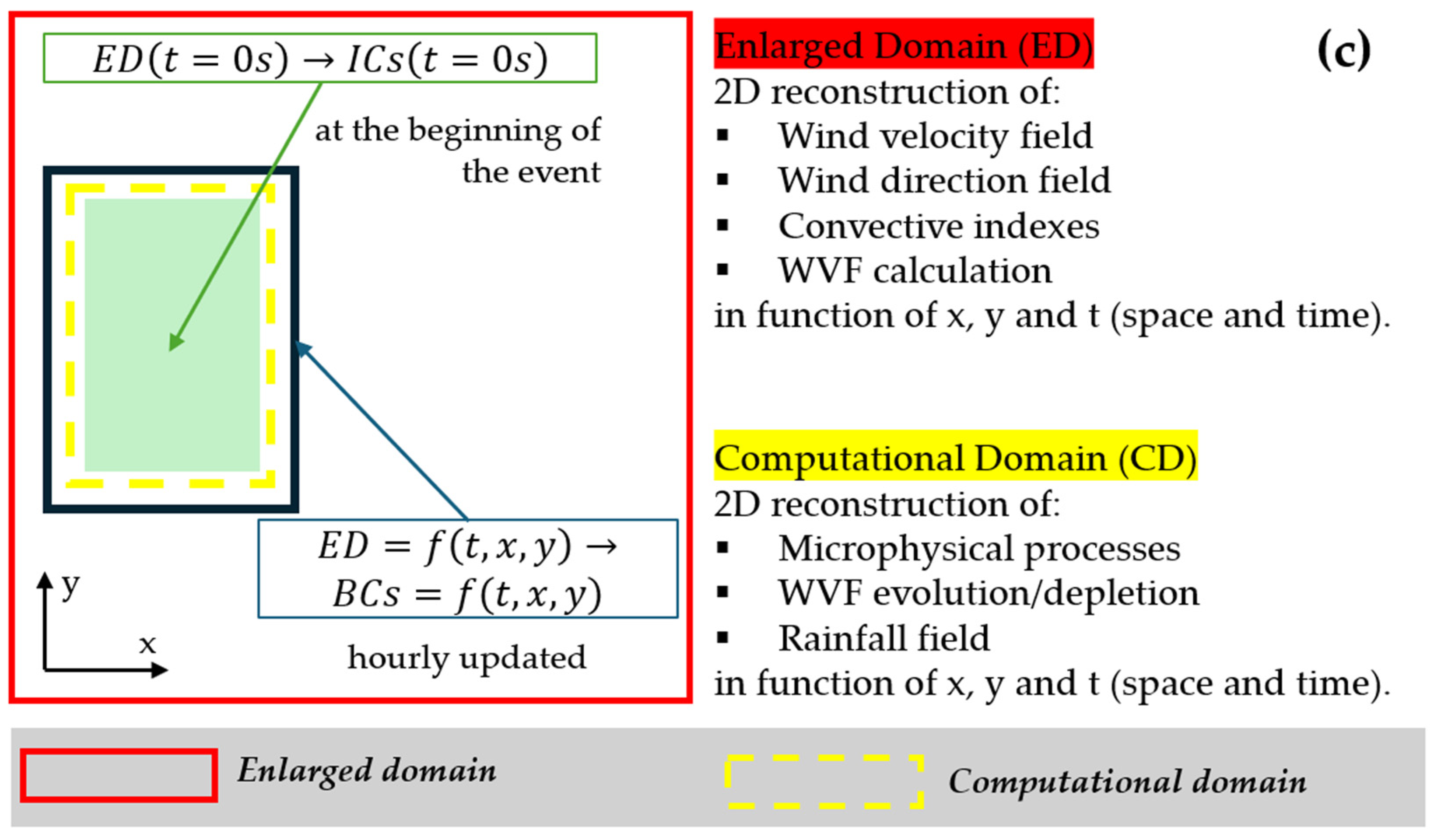
Before running the LUME 2D model, boundary conditions and some key parameters need to be specified within the investigated domain. The latter has a smaller dimension compared to the enlarged domain. Therefore, boundary conditions can be specified in a rather simple way, nesting into the investigated domain the key parameters and the atmospheric variables fields computed for the enlarged domain, using the .netcdf file previously obtained. The model initialisation is carried out by importing the following 3 groups of data as listed in Table 2:
Atmospheric variables: Tref, γ e n v , Γ m o i s t , N m o i s t , ρ r e f , R H r e f , U and D.
Convective parameters: CAPE, CIN, LCL, LFC, EL, PW, PE, G1 and G2.
Boundary-layer height.
Starting from these data, other key variables are derived from the principal ones: WVF (wind vapour flux), Hw (water-scale height) and τc and τf (time-scale parameters for rainfall generation and fallout processes). Since all the variables and parameters are critical, their accuracy is always analysed before the model is run. This passage permits us to assess if the preprocessing has been performed correctly in reproducing realistic time-series of the atmospheric conditions. In the Appendix A, Appendix B and Appendix C, some insights are reported about the convective parameters, τc and τf evaluation and boundary-layer height estimation.

2.2.2. Microphysical Routines

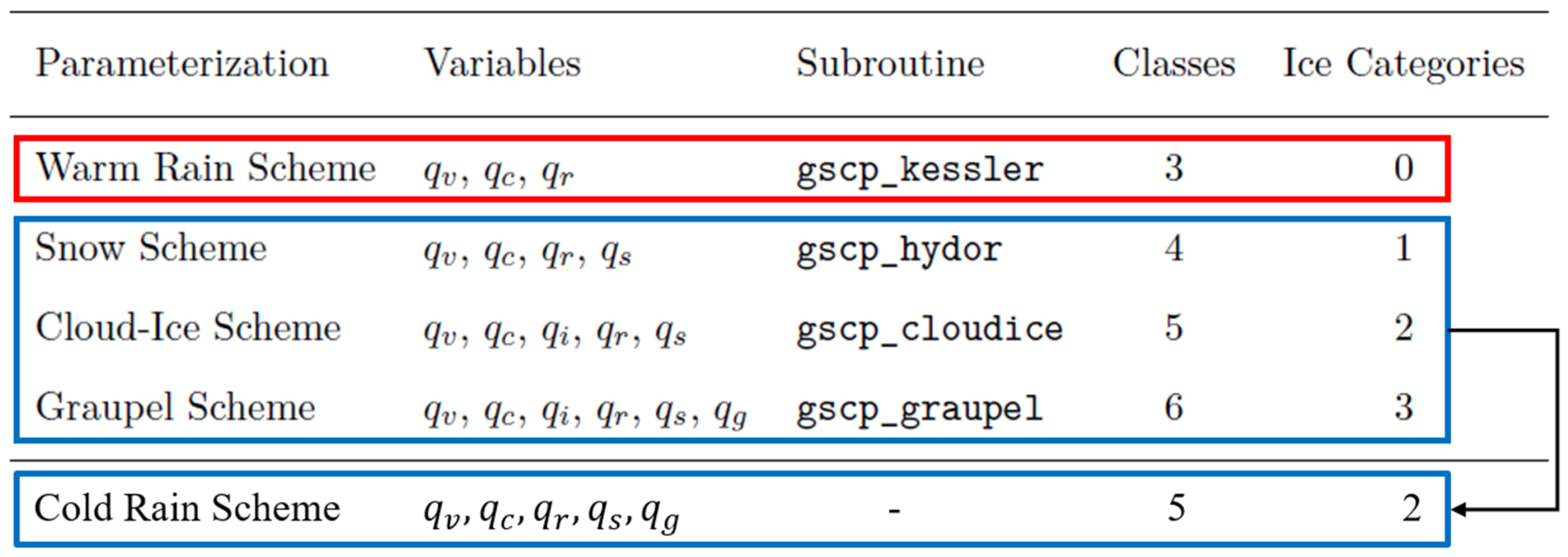
Now, LUME 2D includes a formalisation of the microphysical process according to simple rain schemes elaborated in the literature [30] (Figure 2): two bulk schemes (“warm-rain” and “cold-rain”) are implemented:
In the warm-rain scheme, only 3 microphysical categories are allowed: qv, qc, and qr. They are the same as those proposed in the previous version of LUME, but with a different microphysical parameterisation of the source terms, suggested by the COSMO model.
In the cold-rain scheme, two “cold” categories are added to the system: qh (hail) and qs (snow). The former is a simplification of the full cold scheme proposed in COSMO, where the qi (ice) category has been neglected. This choice was motivated by the fact that the microphysics of ice is highly non-linear and it is difficult to implement straightforwardly, assuring the numerical stability of the code [30].
Warm-Rain Model
The warm-rain scheme is based on the simple Kessler idea [34]. The model is able to compute the evolution in time of the 2 components of the cloud qc and qr in a straightforward way, expressed in mm = l m−2 ≈ kg m−2. qc is the condensed water vapour within the cloud that is provided from the surrounding atmosphere, while qr is the precipitating water (i.e., rain) that is transformed starting from condensate qc. In the COSMO model, these two differential equations are applied for each atmospheric layer and describe the overall cloud mass balance. However, to close the system, two more equations are needed. One describes the qv mass balance, the evolution of the water vapour available in the atmosphere, able to trigger the cloud formation. qv evolution depends mainly on the atmospheric state variables and on their advection through the investigated spatial domain. Their physical transformations (condensation when qv > qc, or conversely evaporation when qc > qv) are able to influence the energetic state of the atmosphere (i.e., local temperature may change due to the latent heat of condensation/evaporation) [42].
With respect to the previous LUME version, now the warm-rain scheme is fully written following the COSMO notation. It is a linear system of partial differential equations (PDE) (1): qv, qc, and qr are variables in space (x,y) and time (t) and represent the vertically integrated cloud vapour, the cloud water, and the hydrometeor densities (in mm ≈ kg m−2). Sources and sinks are functions of the microphysical variables (2), (3), and (4). In Equation (2), the condensation ratio Cw is defined as a product of ρ air, which is the reference density of the atmosphere near the ground, the moist lapse rate Γm (0.0065 °C m−1), and the γ environmental lapse rate. In Equation (4), the water-scale height Hw (or the depth of the moist layer) is defined as a function of Rv = 461 J kg−1 K−1; Tref = reference temperature on the ground, Lv = 2.5 · 106 J kg−1 and γ. Equation (4) expresses the source term in integral form as a function of elevation z. The lower limit corresponds to z1 = LCL (Lifted Condensation Level), while the upper limit corresponds to z2 = EL (Equilibrium Level). The cloud water source Sc is a sum of the upslope condensation [8,23] ( H d e m 0 ) and the eventual super-saturation of the air mass (2); evaporation is calculated separately to condensation only for downslope areas ( H d e m < 0 ) (3), while the microphysical process of accretion and nucleation is simplified according to COSMO model parameterisation (4).
T t = A T + L v c p d   S c S e v q v t = A q v S c + S e v q c t = A q c + S c S a u S a c q r t = A q r S e v + S a u + S a c   P r w h e r e   A q x = U q x   q x U   a d v e c t i o n   t e r m   c o n s i d e r i n g   q x = 0     a n d   P r = q r / τ f  
S c c o n d e n s a t i o n   s o u r c e   + = S u p s l o p e + S C O S M O ( w h e n   q v > q v s a t ) S u p s l o p e = C w H w z 1 z 2 w x , y , t exp z H w d z w h e r e   w x , y , t = U x , y , t H d e m   w i t h   H d e m 0   ( u p s l o p e   w i n d ) w h e r e   C w = ρ r e f Γ m / γ e n v w h e r e   H w = R v T r e f 2 L v γ e n v S d o w n s l o p e = | S u p s l o p e |   w h e n   H d e m < 0   ( d o w n s l o p e   w i n d ) S C O S M O = q v q v s a t τ c o s m o w h e r e   τ c o s m o   1000   s
S e v e v a p o r a t i o n   s i n k   = S d o w n s l o p e + S C O S M O ( w h e n   q v < q v s a t )
S a u + S a u a u t o c o n v e r s i o n   a n d   a c c r e t i o n   s o u r c e   + q c / τ c
Cold-Rain Model
The cold-rain scheme is similar to the warm one but also includes the cold precipitation categories, the qs (snow) and qh (hail). Both are representative of the two opposite seasonalities of the cloud processes. Generally, snow precipitation happens during the winter season and is characterised by smoother rates, even though a significant amount may be accumulated [28,43], especially in the upper parts of the mountains (where temperatures are more frequent when T < 0 °C). Conversely, hail formation is typical of the summer periods [44], where intense storms driven by strong updrafts may hit a mountain range, triggering microphysical processes able to produce it. Hail production is, in fact, a highly non-linear process that is parameterised in COSMO by non-linear equations (not reported for brevity; see [30]). The system of PDE is presented in Equation (5), where 2 more equations for qs and qh have been added. The fallout timescales of snow (τfs) and hail (τfh) categories are slightly different from rain (τfr), since they take into account the different terminal velocity reached by this type of precipitation. According to the literature [6,28], τfs > τfr > τfh, since their terminal velocities are 1–2 ms−1 < 5–6 ms−1 < 10–12 ms−1. Rain, snow, and hail may happen simultaneously, but some weight terms in the function of the ground temperature Tground and updraft intensity w have been included to disentangle the three types. These functions reported in (9) are similar to the one proposed by the COSMO parameterisation, but simplified. The sources Sv (6) and Sc (7) are the same as the warm-rain scheme.
T t = A T + L v c p d   S c + S r + L s c p d   S h + S s q v t = A q v + S v q c t = A q c + S c q r t = A q r + S r P r q s t = A q s + S s S n q h t = A q h + S h H l w h e r e   A q x = U q x   q x U   a d v e c t i o n   t e r m   c o n s i d e r i n g   q x = 0   a n d   P r = q r τ f r ,   S n = q s τ f s ,   H l = q h τ f h τ f r = r a i n   f a l l o u t   t i m e s c a l e τ f s = s n o w   f a l l o u t   t i m e s c a l e   τ f r · 2 τ f h = h a i l   f a l l o u t   t i m e s c a l e   τ f r / 2  
S v v a p o u r   s o u r c e = ( S u p s l o p e d o w n s l o p e + S C O S M O )
S c c o n d e n s a t e   s o u r c e = + ( S u p s l o p e d o w n s l o p e + S C O S M O ) q c / τ c    
S r r a i n   s o u r c e = q c τ c   w h e r e   T g r o u n d > 0   ° C
S s s n o w   s o u r c e = q c 2 τ c   w h e r e   T g r o u n d < 0   ° C   a n d   w x , y , t 0   ( w e a k   u p d r a f t ) S h h a i l   s o u r c e = q c 0.5 τ c w h e r e   T g r o u n d < 0   ° C   a n d   w x , y , t 0   ( s t r o n g   u p d r a f t )                             P s t o n g   u p d r a f t = 0.2 w x , y , t 0.5 e m p i r i c a l
Numerical Integration
Even if the warm-rain and the cold-rain schemes are linear systems of PDE, their solution was not computed analytically but integrated numerically using the “upwind” numerical method [45]. The upwind method is a numerical technique used to solve advection equations, frequently adopted in computational fluid dynamics. It approximates derivatives in the direction of the flow (the “upwind” direction) determined by the advection equation. This method has been revealed to be rather powerful in maintaining good stability in the integration with respect to a temporal-adaptive timestep that was addressed by verifying the stability condition of the Courant number [45,46]. The explicit “upwind” method was selected for the sake of simplicity, but other numerical methods (such as the implicit ones) could be considered to avoid the constraint imposed by the stability condition. Simple upwind schemes are typically only first-order accurate in space, meaning they have a relatively large truncation error. Higher-order upwind schemes can be developed to improve accuracy; however, they might be more complex to implement [47].

2.3. Atmospheric Convection

The third innovation included in the 2D LUME model is the ability to interpret the moist convection within the warm-rain or the cold-rain microphysical schemes. Moisture convection is a process that leads to thunderstorm cell formation, which is very different from stratiform precipitation (i.e., the type modelled by LUME) [6]. Thunderstorms and associated convective precipitation are spatially localised, exhibit higher rainfall ratios, and last for a few hours (typically, if regenerative thunderstorms are excluded) [3,5]. Moisture convection is triggered by intense updrafts that could be thermally induced (due to the boundary-layer processes), mechanically induced (orographic lift) or caused by a frontogenesis mechanism [24,48]. These processes are distinguished in the literature, but often they happen simultaneously, leading to difficulty in interpreting the thunderstorm formation and evolution. Moisture convection involves a high amount of energy exchange that can also perturb the microphysical processes [6]. Therefore, the possible energetic feedback caused by energy and heat exchanges within microphysical processes cannot be fully neglected [24].
The scope of this work does not aim to solve the convection mechanism explicitly but tries to find a way to include it within the upslope model, keeping a reasonable physical interpretation. Therefore, two components were added to the previous rain-scheme specifying when and where convective rainfall may activate, contributing to the total rainfall:
When: The triggering functions to determine when the convection may activate during a storm are available in the literature [49]. Using the convective parameters or a combination of them, these functions can detect when moist convection may develop. These functions could be continuous or discrete, but generally are represented as a critical value (threshold) of a specific convective index (CI). If |CI|< threshold, moist convection does not occur, while if |CI| ≥ threshold, it is likely to start. In Table 3, the convective indices are specified (CAPE, CIN, LI, KI, SI and DCI) and the relative thresholds are applied in this study according to the indications in the literature [49].
Where: Triggering functions can be applied at each radiosonde location simply by considering the local estimation of the convective indices. However, due to the significant spatial variability of CI (stations may lie several hundred kilometres apart, experiencing different convective environments), it is advisable to carry out the study considering a spatial interpolation of the convective parameters. This could help determine the location where moist convection is more likely to occur, i.e., when the CIs overcome the triggering thresholds.
Knowing when and where the moist convection occurs, the probability of its activation can be estimated. The probability function retrieved from each CI is a simple normalisation of the index between the “threshold maxima” and its minimum. Therefore, when the index exceeds the threshold, the probability of triggering convection becomes = 1. The necessity of normalisation comes from the fact that every triggering function has its own history and has been elaborated under certain conditions, using a particular model, where thresholds and mathematical formulations may be very different [24]. Therefore, trying to compare different triggering functions is not always feasible when keeping the “original” formulations, but it is necessary since each function can describe or emphasise a certain aspect of convection (total energy, thermal profile, etc.) which may contribute to increasing the probability of moist convection occurring. Bearing in mind this fact, for each timestep and for the enlarged domain, the continuous convective triggering functions have been normalised between 0 and 1 and then averaged together (see Equations (10) and (11)) for the probability. In particular, pconv1 was calculated considering only the CAPE and CIN “energy related” index in their normal and “virtual” versions (using virtual temperature), and pconv2 was calculated for the other “operative” indexes LI, TT, KI, SI, and DCI, normally adopted in thunderstorm forecasts. Then, the two probabilities have been averaged together, retrieving the unique indicator pconv for moist convection triggering. The latter has been evaluated at each timestep of the model, considering the temporal interpolation of each CI. Namely, a probability of 0.8 (80%) states a favourable situation for starting convection, while with 0.3 (30%), it may not occur properly. These probabilities have been exported in a .netcdf file.
p c o n v 1 = ( p C A P E + p C I N + p C A P E v + p C I N v ) / 4
p c o n v 2 = ( p L I + p L I v + p T T + p K I + p S I + p D C I ) / 6
p c o n v = ( p c o n v 1 + p c o n v 2 ) / 2
In addition, boundary-layer convergence and upper-layer divergence were calculated as a proxy for moisture convection activation [3]. These highlight how the wind dynamics at the synoptic scale in the lower and upper troposphere can enhance/reduce the vertical updraft velocity. Equations (13) and (14) are based on the continuity equation of horizontal flows impinging on the ground (i.e., boundary-layer pumping) to the upper layers, where jet stream acceleration may happen [15]. Therefore, the Wmid-BL and Wmid-JS (expressed in ms−1) have been considered to calculate the probability pwind (15) of moist convection due to enhanced updraft.
W m i d B L = C o n v B L · H e i g h t B L B L   u p d r a f t C o n v B L = U x B L x + V y B L x
W m i d J S = D i v g J S · H e i g h t J S J S   u p d r a f t D i v g J S = + U x J S x + V y J S x
p w i n d = ( W m i d B L + W m i d J S ) / m a x ( W m i d B L + W m i d J S )
Up to this point, the magnitude of the rainfall associated with moist convection still needs to be defined. The Magnitude of the convection source has been established from [35], following the one-dimensional cloud model proposed by Kessler [34]. The simple idea is that the strength of the moisture convection is a function of the updraft velocity w that could, in principle, be estimated starting from some convective parameters [44]. Therefore, in the absence of convection (i.e., when convective parameters have their lowest value), updraft velocity is negligible and the contribution to the “stratiform” source term is close to zero. Equations from (16) to (19) report the calculation of “convective magnitude” as a function of the maximum updraft calculated for CAPE and CIN convective indexes, expressed in J kg−1. Gi functions also depend on convective heights EL and LFC (m), which are characteristics of the moist convective environment [34]. Gconv is the mean of G1 and G2, and is expressed in mm h−1. As presented here, the moist convection that contributes to precipitation is described at grid bases (the same resolution of the DEM), not explicitly resolving the sub-grid moist convection. The Gconv function is established considering a “mean vertical state” of the atmosphere. However, to be resolved explicitly, sub-grid moist convection should take into account the vertical profile of the atmosphere and a higher DEM resolution (namely <1 km, at least) [6,24], which conflicts with the purpose of keeping LUME 2D simple. Moreover, the energy balance (i.e., CAPE closure [50]) is not considered at this level of the model development, though it is a “necessary” assumption in order to solve the moist convection evolution and dissipation mechanisms that may occur at sub-scales. Further details about the possible improvements of LUME 2D in representing moist convection are also reported in the Discussion section.
g 1 = c 4 · E L + ( c 5 · E L 2 ) / 2 g 2 = c 4 · L F C + ( c 5 · L F C 2 ) / 2 w h e r e   c 4 = 3   10 3   a n d   c 5 = 3   10 7
w m a x 1 = 2 · C A P E 0.5   w i t h   C A P E > 0   J k g 1 w m a x 2 = 2 · ( 100 + C I N ) 0.5   w i t h   C I N < 0   J k g 1
G 1 = 0.6 · w m a x 1 · g 1 g 2 G 2 = 0.6 · w m a x 2 · ( g 1 g 2 )
G c o n v = ( G 1 + G 2 ) 2
Knowing the location, the timing, and the magnitude of the moist convection source, the strategy employed to include it within the LUME 2D model is described. This was a challenging aspect that has been resolved by looking at the mathematical structure of the model, which is a linear system of PDEs [30]. Keeping in mind that one of the properties of linear systems is the superimposition of the effect [47], the final solution of the system (i.e., the total precipitation) can be obtained in principle by adding to the “stratiform-orographic” solution the “convective” one. But how? The choice made in 2D LUME was to add to the upslope source (Supslope triggered by mechanical uplift) the additional term Gconv weighted by the probability pconv. In this way, the convection term remains a spatially and temporally dependent term which can intensify the precipitation when it is activated. This choice aims to keep the convection contribution mathematically tractable, simple to understand, and straightforward to implement. Equations (20) and (21) show the inclusion of the convective term into Sc sources for warm-rain and cold-rain schemes. Existing interferences among the stratiform and convective evolution of the source have been neglected, considering only the storm intensification due to the presence of convection [6,9,24,44,51,52].
f o r   w a r m r a i n   s c h e m e S c ( W R + m o i s t   c o n v e c t i o n )   = S u p s l o p e d o w n s l o p e + S C O S M O + G c o n v q c t = A q c + S c S a u S a c + S c o n v S c o n v = p c o n v · G c o n v
f o r   c o l d r a i n   s c h e m e S c ( C R + m o i s t   c o n v e c t i o n )   = S u p s l o p e d o w n s l o p e + S C O S M O + G c o n v q c t = A q c + S c + S c o n v S c o n v = p c o n v · G c o n v  

2.4. Data Analysis

Any model requires an accurate revision of the results to spot possible errors or bad parameter conditioning. In this paragraph, LUME 2D performance was evaluated through an error analysis. The results (i.e., rainfall amounts, microphysical quantities, sources, etc., at each timestep) are reported as a matrix stack in .netcdf formats. After any simulation, they can be saved and then compared to the reference rain-gauge series recorded within the investigated domain. Sampling the .netcdf files at the reference rain-gauge location, a “global statistic” and a “local statistic” analysis on simulated rainfall series have been developed.

2.4.1. Global Statistics of the Total Rainfall Field

Global error statistics are evaluated considering the total rainfall field calculated at the end of the simulated event (Pmod) and using the total rainfall cumulated at each reference rain gauge (Pref). This analysis is similar to the one reported in [23], and its aim is to highlight whether the spatial distribution of the modelled rainfall field is in accordance with the rain-gauge recordings across the territory. In this light, the “global error indices” reported in Equations (25)–(27) have been calculated by comparing Pref and Pmod [23]. BIAS represents the absolute error, evaluating the offset between the reference and the predicted quantities. RMSE is the Root Mean Square Error and measures the differences between true or predicted values on the one hand and observed values. AIS is All Indicator Scores, which is the sum of the BIAS and RMSE, evaluating both considering additive and multiplicative error models. They are expressed in mm.
The comparison has been carried out considering two types of error models: the additive and multiplicative [53,54]. According to [53], the additive model (22) is generally applied with variables characterised by a Gaussian distribution (such as the temperature) where median and mean are very close together. On the other hand, multiplicative error (23) is suitable for log-normal distribution (such as rainfall intensity), where median and mean could be significantly different depending on the dataset analysed. A linearised version of the multiplicative errors consists of converting Equation (22) with logarithms (24), again obtaining an additive error model of the logarithm of the investigated quantities. However, the two error models (additive and multiplicative) have been kept separated in the analysis.
Y i = a + b · X i + ε
Y i = a · X i b e ε i
l n ( Y i ) = ln a + b · l n ( X i ) + ε i
Other “normalised” indices (i.e., with 0–1 scale) have been tested in the analysis [29,55]. The Mean Absolute Percentage Error (MAPE) is a measure of prediction accuracy. Due to some inconsistencies when the data approaches 0 (it cannot be used if there are zero or close-to-zero values, because this would involve a division by zero or values of MAPE tending to infinity), the SMAPE was evaluated instead (28). The Symmetric Mean Absolute Percentage Error (SMAPE) is a statistical measure used to assess the accuracy of predictions that considers both overestimation and underestimation by comparing the absolute difference between actual and predicted values to the average of their absolute values. A lower SMAPE indicates a more accurate prediction: the resulting score ranges between 0 and 1, where a score of 0 indicates a perfect match between the actual and predicted values, and a score of 1 indicates no match at all. The correlation coefficient (CC) measures the model’s ability to predict precipitation patterns, independent of magnitude, and gives a score between 0 and 1 (29). According to [29], a reference value for C C r e f   is 0.637. If C C > C C r e f , the model results and observations are significantly correlated. Perfect pattern agreement between data and model would give C C = 1.
B I A S a d d = 1 n i = 1 n P r e f P m o d           B I A S m u l = 1 n i = 1 n ln P r e f l n ( P m o d )
R M S E a d d = 1 n i = 1 n P r e f P m o d 2   0.5       R M S E m u l = 1 n i = 1 n ln P r e f l n ( P m o d ) 2   0.5
A I S = B I A S a d d + B I A S m u l + R M S E a d d + R M S E m u l
S M A P E = 1 n i = 1 n P r e f P m o d P r e f + P m o d 2
C C = i = 1 n ( P r e f + P m o d ) / i = 1 n P r e f + P m o d 2 0.5  

2.4.2. Local Statistics on a Single Rain Gauge

Error statistics can also be evaluated for each station. The rainfall intensity (I) and the rainfall cumulated (C) evolution during the event can be compared to corresponding rain-gauge measurements, showing whether the temporal evolution of the model reconstruction was consistent with reality. The following error statistics have been evaluated for Pref and Pmod, considering both the rainfall intensity and the cumulated series [56]. The Nash–Sutcliffe Efficiency (NSE) is calculated as one minus the ratio of the error variance of the modelled time-series divided by the variance of the observed time-series (30). In the situation of a perfect model with an estimation error variance equal to zero, the resulting Nash–Sutcliffe Efficiency equals 1 (NSE = 1). Conversely, a model that produces an estimation error variance equal to the variance of the observed time-series results in a Nash–Sutcliffe Efficiency of 0.0 (NSE = 0). NNSE is a rescaled NSE that lies solely within the range of [0, 1]. Note that NSE = 1 corresponds to NNSE = 1, NSE = 0 corresponds to NNSE = 0.5, and NSE = −∞ corresponds to NNSE = 0. The Kling–Gupta Efficiency (KGE) is a goodness-of-fit indicator, where r is the Pearson correlation coefficient, α is a term representing the variability of prediction errors, and β is a bias term (31). The KGE ranges between −∞ and 1, where a value of 1 indicates perfect agreement between the model predictions and the observed data. NKGE is a normalised version of KGE (similar to NNSE) where the range is rescaled between [0–1].
N S E = 1 i = 1 n P r e f P m o d 2 P r e f P m o d ¯ 2 P m o d ¯ = 1 n i = 1 n P m o d N N S E = 1 2 N S E
r = 1 n   i = 1 n P m o d P m o d ¯ · P r e f P r e f ¯ v a r P m o d 0.5 · v a r P r e f 0.5 P r e f ¯ = 1 n i = 1 n P r e f α = P m o d ¯ / P r e f ¯ β = v a r P m o d 0.5 / v a r P r e f 0.5 K G E = 1 r 1 2 + α 1 2 + β 1 2 0.5   N K G E = 1 2 K G E

2.5. Case-Study Description

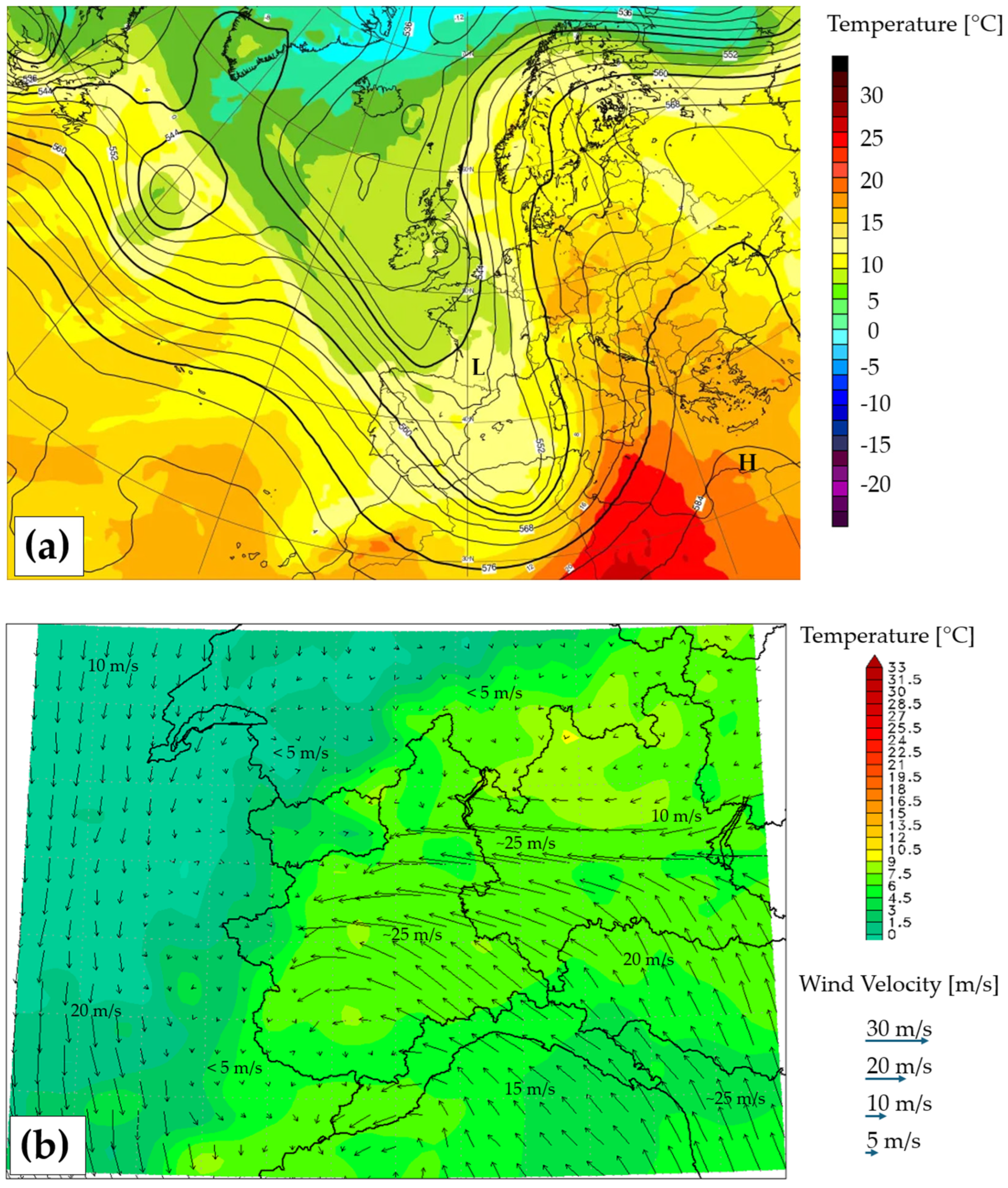
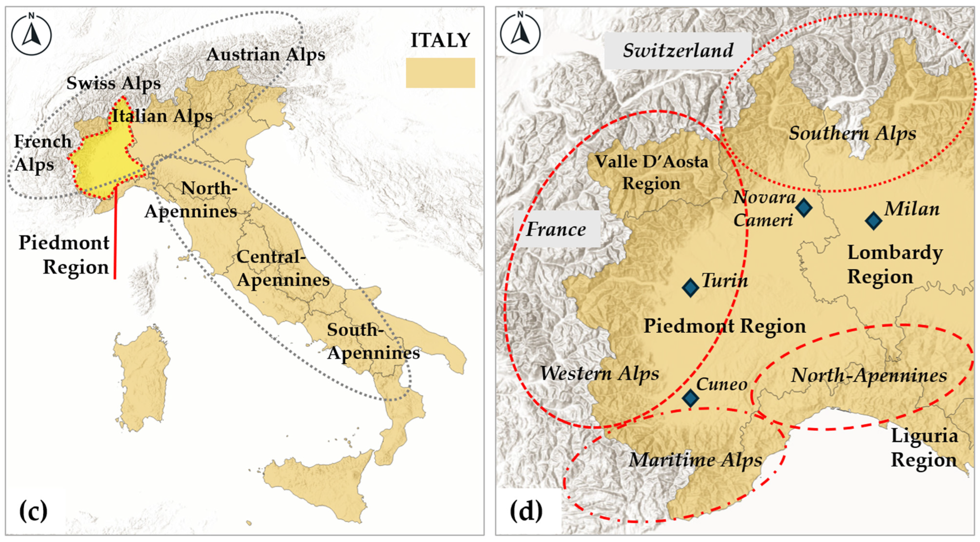
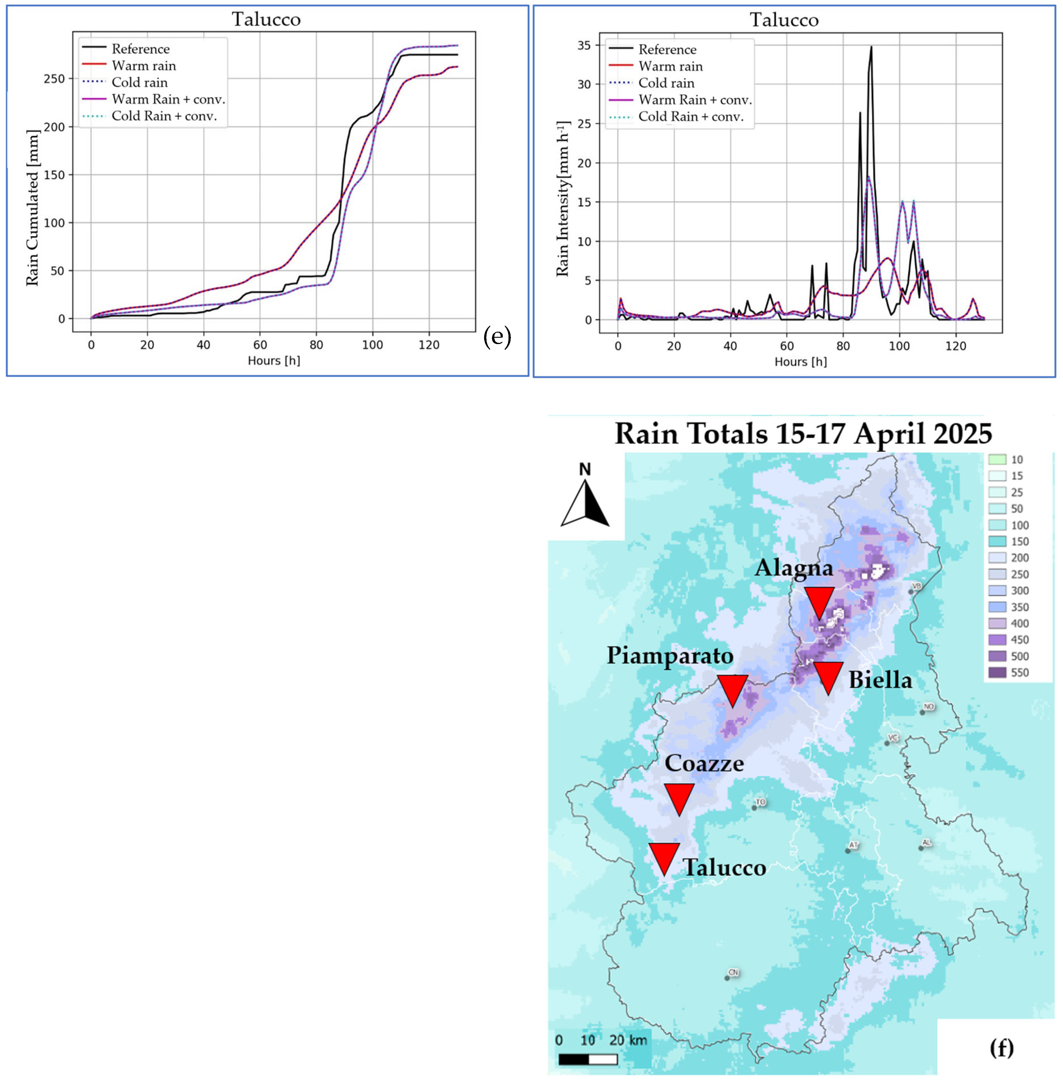
The LUME 2D model was extensively tested on a southern alpine orographic precipitation event that hit the area of Piedmont (Figure 3c,d), in Italy, during spring 2025 [31,32]. Between the evening of Tuesday 15 and Thursday 17 of April 2025, an intense sirocco episode—linked to the deepening of the “Hans” depression over the Ligurian Gulf—produced the most copious rainfall in northwest Italy. The intense perturbed episode involved a preparatory phase over the previous few days, first with a predominantly Atlantic matrix and modest phenomena. Then, a Mediterranean component exacerbated the supply of humid air towards the south of the Alps with the activation of very intense phenomena. From Monday 14 April, the descent of the cold air mass from the North Atlantic to the western Mediterranean continued to feed the humid advection towards the Alpine regions with currents at high altitude first from the south, then from the southeast. From this secondary cyclogenesis, the minimum pressure, called “Hans”, a vortex responsible for the most acute phase of precipitation, was formed [31] (Figure 3a). Over the course of 24 h between Wednesday 16 and Thursday 17 April, the ground pressure between the coasts of Western Liguria and the Côte d’Azur dropped from 1008 to 1010 hPa to 991 hPa, with an almost “explosive” cyclogenesis that activated strong easterly winds from the upper Adriatic towards western Piedmont (Figure 3b).
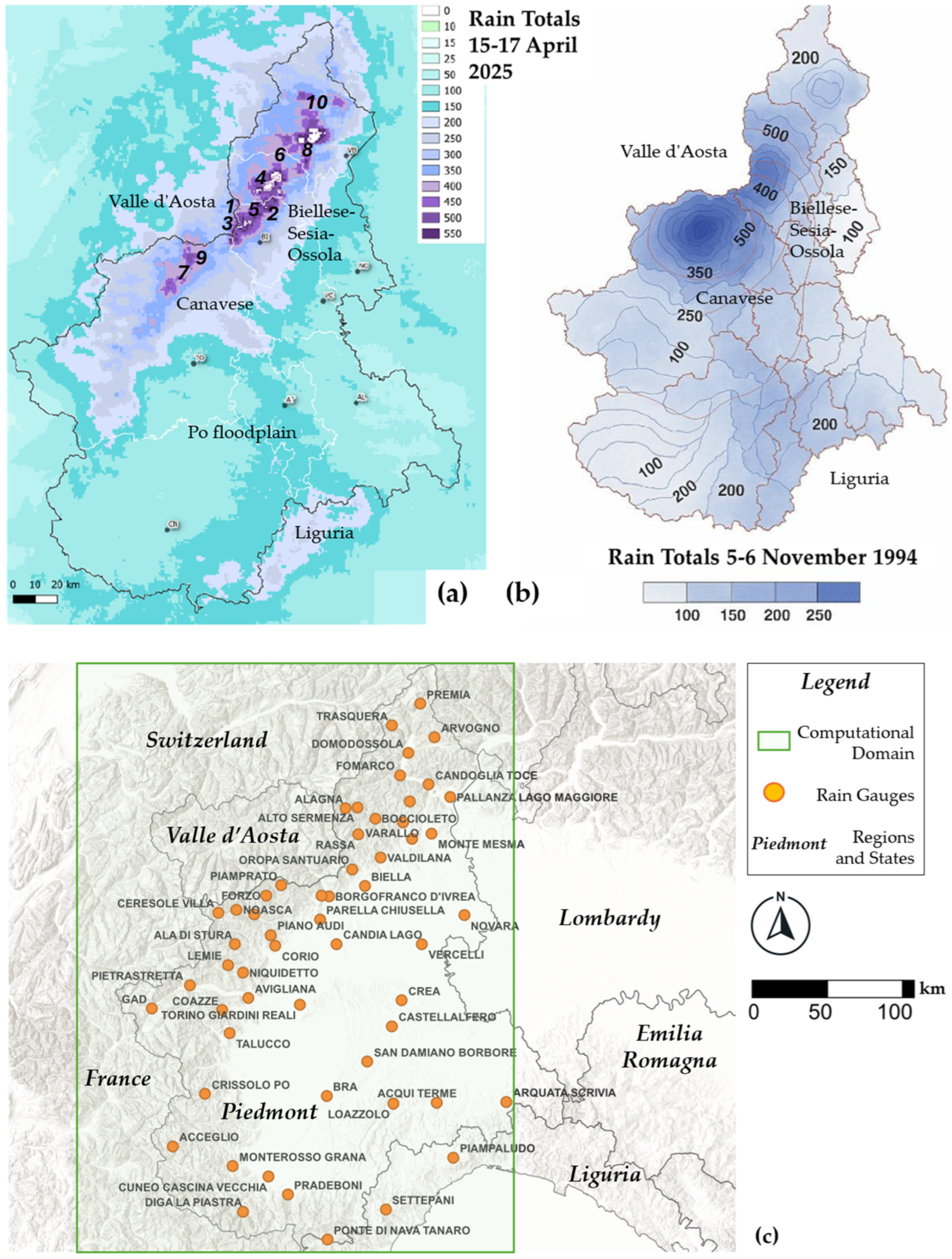
The event lasted 72 h (around three days) and was characterised by a huge amount of rainfall that fell locally in the Northern Piedmont Alps (in the Biella and Verbania provinces). Huge quantities of rain, up to over 400–500 mm on the reliefs between the upper Canavese, lower Valle d’Aosta, and Biellese-Sesia-Ossola (sometimes recorded over intervals of 1–2 days) had a heavy impact on the territory, with large watercourse floods (especially of the Po River and its tributaries), widespread overflows and floods, landslides, and debris flows on roads and hill and mountain settlements. Focusing on the areal distribution of rainfall, the event shows even greater similarities with what happened in 1994, albeit with much lower quantities in the areas bordering Liguria (Figure 4). The total rainfall field-recorded at the end of the event exhibits a sharp gradient of cumulates if the floodplain and the Alps ranges are compared, as reported in [31,32]. The rainfall was characterised by persistent rainfall rates but also convective episodes, and snow thunderstorms were recorded, making the event rather complex and variegated (Table 4).

3. Results

In this section, the results obtained from LUME 2D tests are reported, carrying out the rainfall reanalysis of the event of April 2025. All the time-series show the x-axis ranging from 0 to 144 h, which corresponds to the period from 13 to 18 April 2025. The investigated rainfall event occurred between 48 h and 120 h, corresponding to 15–17 April 2025.

3.1. Two-Dimensional Data: The Wind Influences the Event Strength

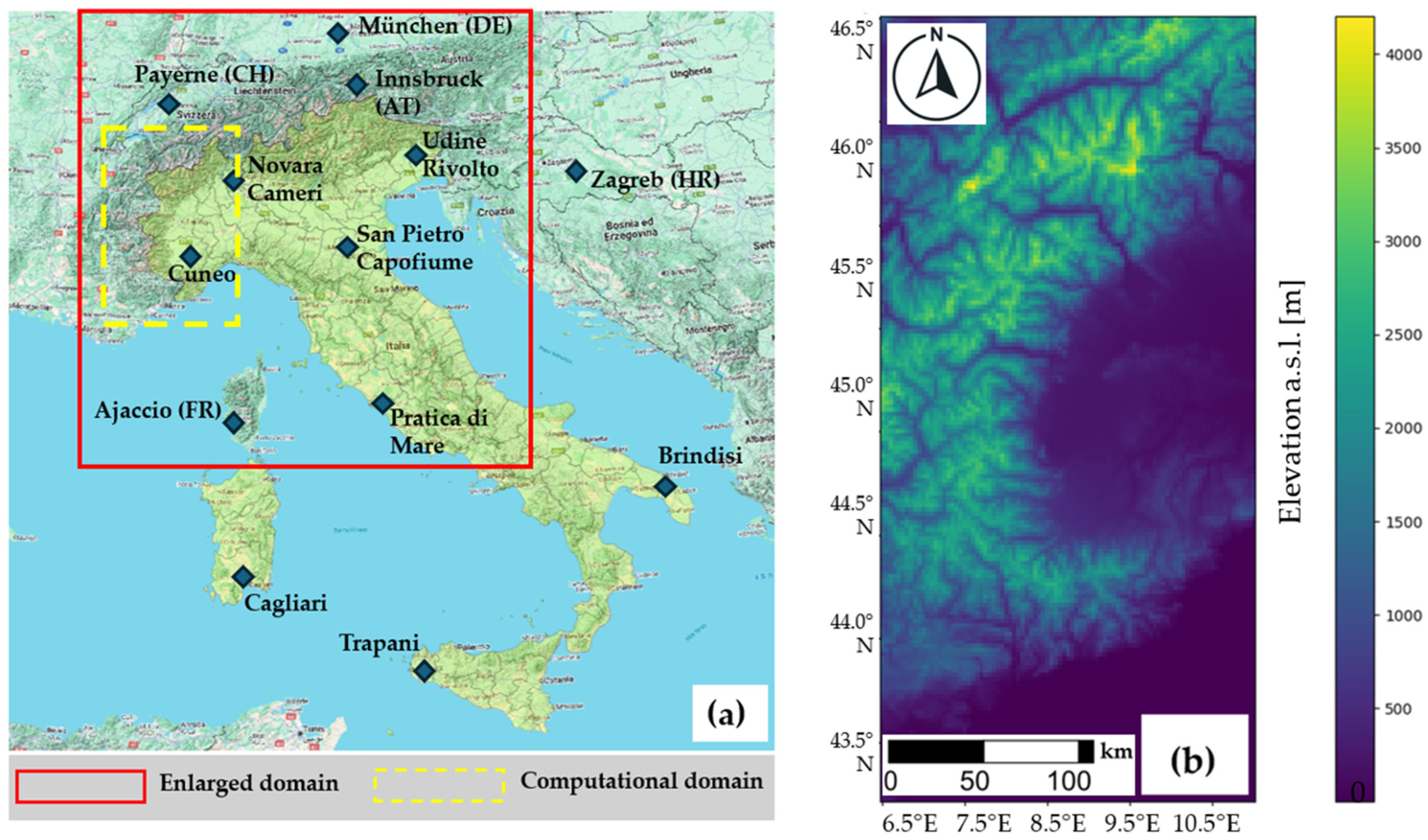
Two-dimensional data are necessary to feed the model, and two spatial domains are required for computation. The first one, called “investigated domain”, should relate to the area of investigation (in this case, the Piedmont area in northwestern Italy), while the second should be an “enlarged domain” useful for spatial interpolation of radiosonde stations. In Figure 5a, the two domains are represented: red box > enlarged domain and yellow box > investigated domain. The latter is considered for clipping the digital elevation model (DEM) necessary for the upslope wind-component calculation. DEM has a spatial resolution of 2 km and was resampled from [57] (Figure 5b). The resampling method adopted to reduce uncertainties is the “nearest neighbour”. Nearest-neighbour interpolation is a simple, fast, and efficient method for estimating unknown data values within a dataset by assigning the value of the closest known data point to the new location [58]. It is the default method adopted in the “gdal-functions” implemented in the GIS environment [59]. The interpolation method has appeared to be sufficient to pass from 90 m to 2000 m, not losing accuracy in reproducing mountain range features (principal valleys and peaks) and not introducing algorithm artefacts.
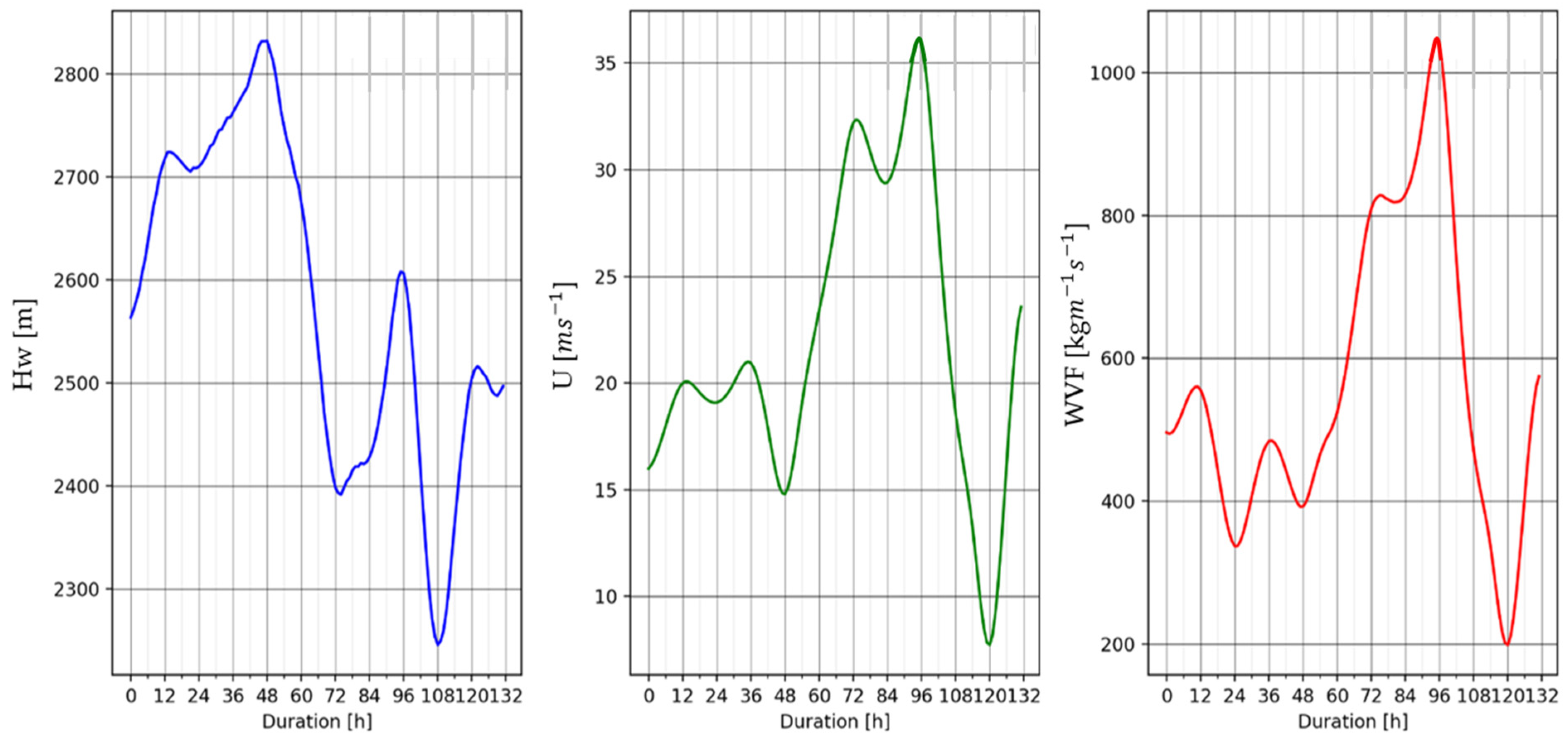
For atmospheric variable and parameter reconstruction, both southern and northern radiosonde stations across the Alps range were spatially and temporally interpolated. As can be observed, the radiosonde location is rather spatially uniform. Particular attention was paid to the reconstruction of the wind velocity and wind direction fields, which exhibit higher spatial variability and gradients. An accurate description is required to avoid under- or overestimation of WVF. The WVF quantity (water vapour flux) and its spatial derivation are representative of the advection of water vapour flux through the calculation domain (see the second equations of the PDE systems (1) and (5)). As described by [7], WVF depends strongly on PW magnitude and vertically integrated U. PW variation (in Equation (33)) is rather smooth since it depends indirectly on temperature T and RH through qv (32); vertically integrated U may be a significant variable in space and along the vertical dimension Even though other terms of the equation may be influential, wind plays a major role in defining WVF magnitude (34), conditioning orographic upslopes in triggering the most intense rainfalls.
q v a p o u r = q v = 0.622 e p e   w h e r e   e = R H   e s ( T )
P W = 1 ρ w a t e r g z = 0 m z = E L ρ v a p o u r d z 1 g p = 1 a t m p = 0 a t m q v a p o u r d p
W V F = ρ a i r H w U = P W   U H w = P W / ρ a i r
In Figure 6 the Hw, vertically averaged U, and WVF terms for the investigated event are reported. As can be observed, the peak of WVF was recorded during the principal phase of the event and lasted 48 h from 15–17 April 2025. These data come from the radiosounding station of Novara Cameri (ex Milano Linate), which is the closest one to the Piedmont area and is located upwind (see Figure 5a). The peak of WVF is synchronous with respect to U, which exhibits a significant increase during the central phase of the event according to [31], while Hw shows a smoother variation.

3.2. Synoptic and Convective Data: Probability and Magnitude

Convective data analysis was carried out using a combination of atmospheric variables and parameters evaluated from 2D interpolated data. In Figure 7, some wind-dependent variables are reported, which have been calculated in order to assess the area of wind convergence and divergence both in the lower (BL—boundary layer) and upper levels (JS—jet stream) of the troposphere. The behaviour is quite different between the two levels, but during the central phase of the analysed event (16th of April), the vertical velocity updrafts calculated from BL and JS (Wmid-BL and Wmid-JS) were recorded as positive across the Piedmont area, highlighting a possible significant contribution of the synoptic configuration to air-mass condensation.
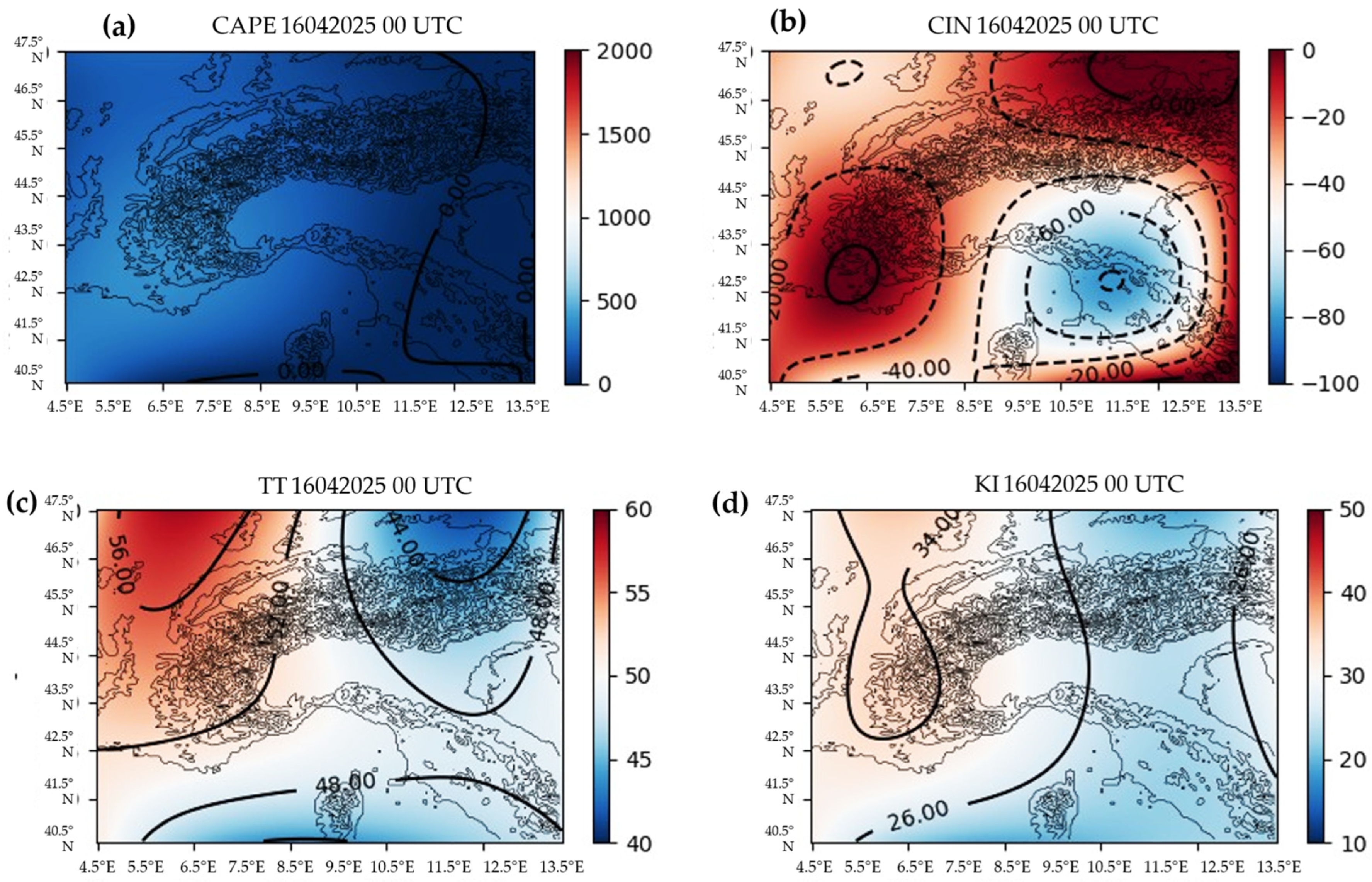
In Figure 8, the convective indexes are shown. The signals able to promote and trigger moist convection are well depicted in a 2D field: even if CAPE is not so pronounced (that is normal if we consider the spring season), TT and KI are quite high, and also CIN (that exhibits an inverse scale) is in agreement, showing a possible favourable condition for local convections across the Piedmont. The same analysis was carried out for other convective indices, LI, SI, etc., (not reported for brevity), showing similar results.
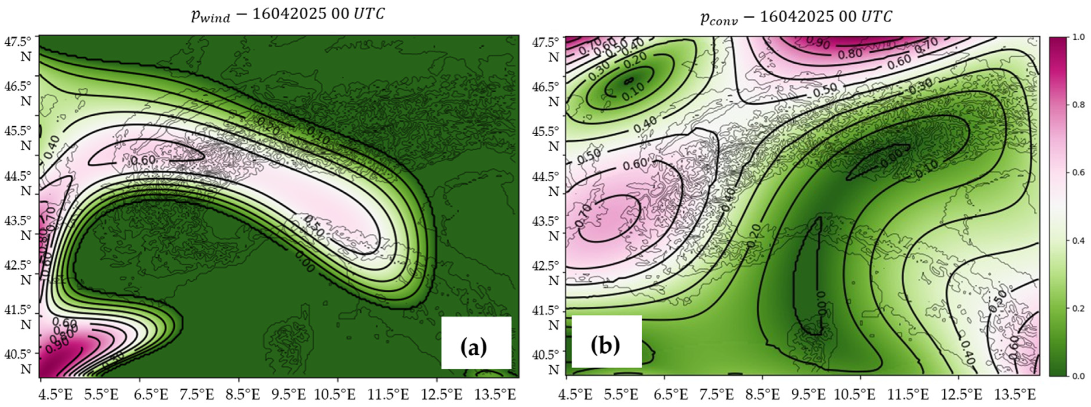
The synoptic winds and the convective index have been merged to compute the probability of moisture convection (Figure 9). After normalisation, the data were averaged, obtaining a depiction of the probability, which has shown (consistently with the single-parameter investigation) a favourable convective environment between the 15th and 17th of April. Magenta areas are those where the probability of moist convection is the highest: for pwind and pconv, moist convection is likely to occur across the Piedmont area, in accordance with the evidence of the meteorological analysis. As can be noticed, the spatial and temporal evolution of convective parameters and triggering functions is quite variegated, and strong gradients are expected across the domain.
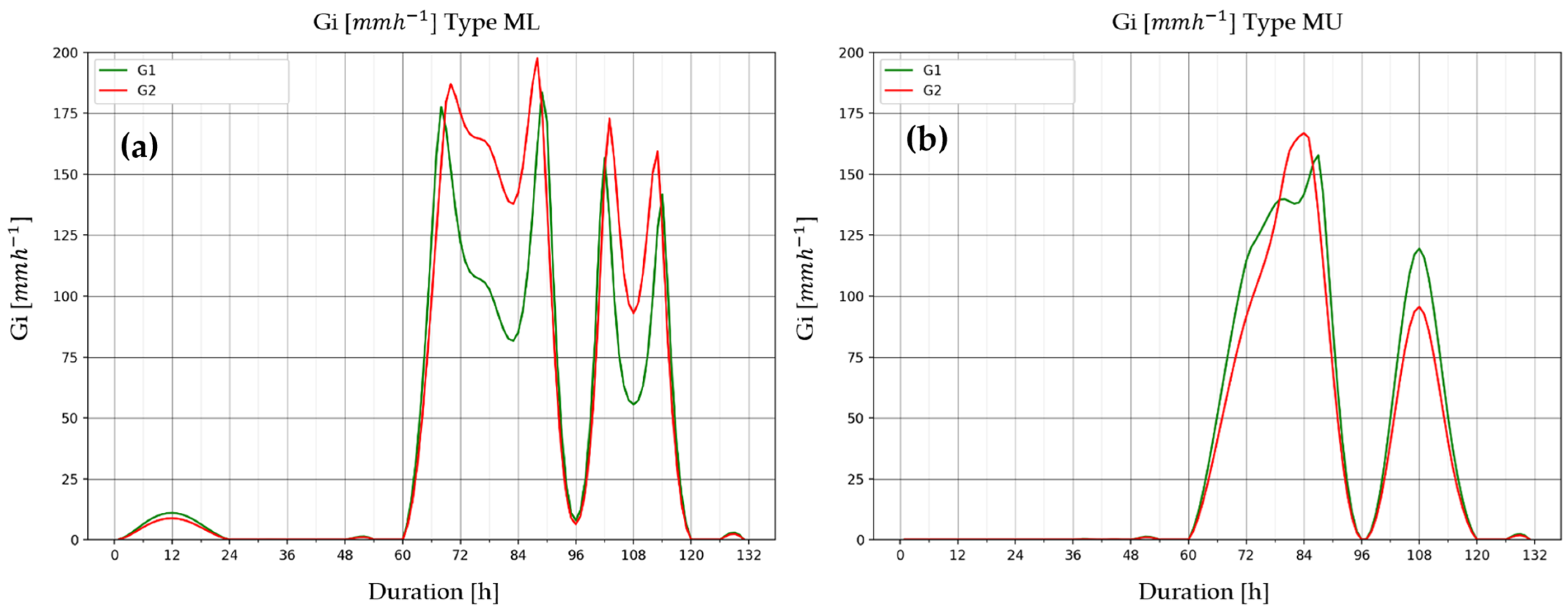
The moist convection magnitude has been evaluated by computing the Gi value under the two scenarios, ML and MU. These two scenarios consider different situations of the “raising particle” method for estimating the convective height LFC and EL: mixed layer (ML) and most unstable (MU) [3,5,6]. As can be observed, the differences are rather small: ML and MU are similar in magnitude (the terms G1 and G2 reach up to 150–200 mm/h), and are representative of the two main phases of the event (occurring between the 15th and 17th of April). Looking at Figure 10a, the ML shows a double-peak graph, while the MU (in Figure 10b) is similar but much smoother. The subsequent computations have considered the ML condition (i.e., the critical one) for Gi calculation.

3.3. Initial Conditions

In this section, the initial conditions computed for the 2D LUME model are presented in three main groups: precipitation efficiencies, conversion and fallout time-scale parameters, and boundary-layer characterisation.
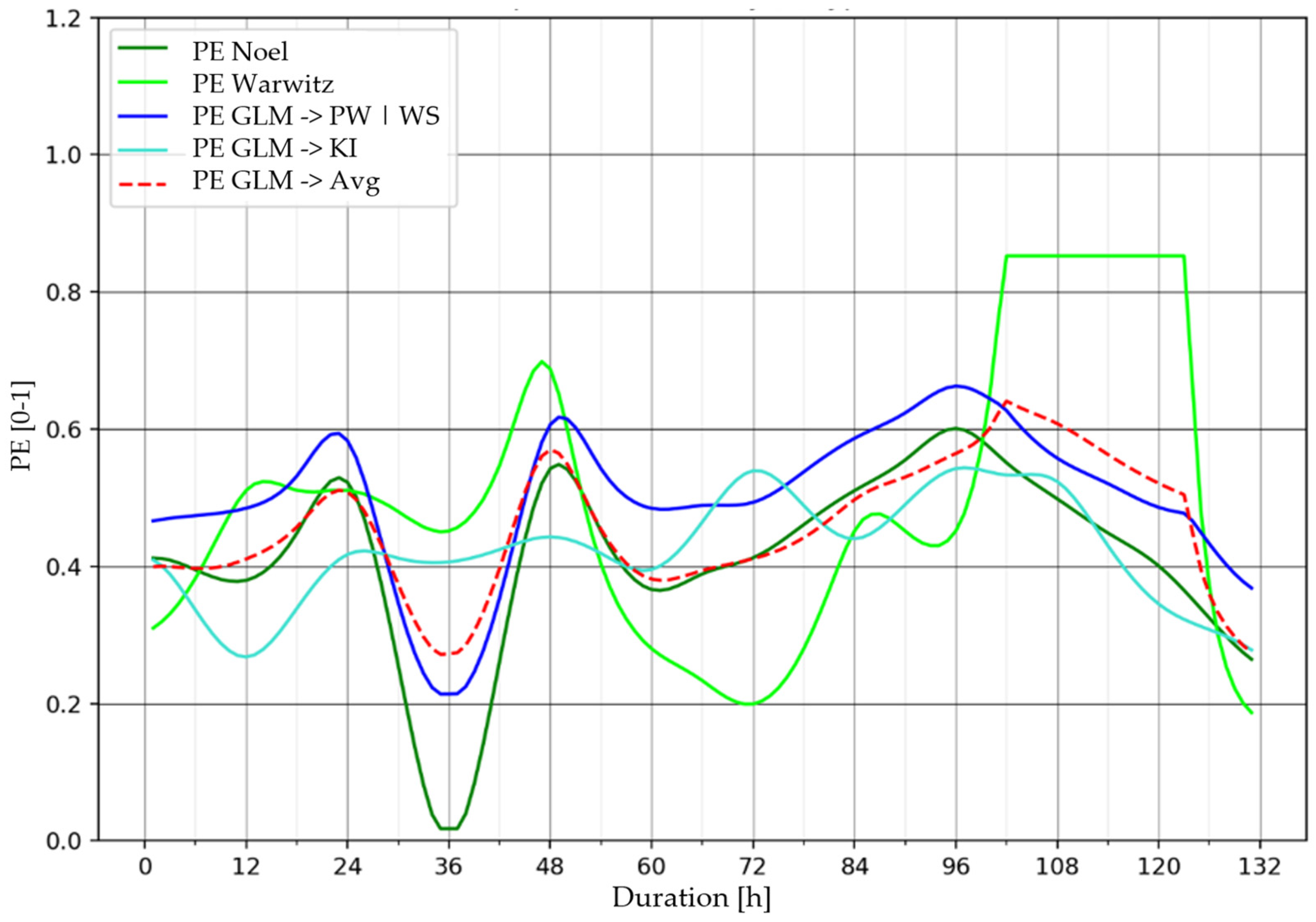
Precipitation efficiency is a parameter that could be, in principle, estimated from the analysis of the radiosonde [26]. In Figure 11, the time evolution of the PE during the event for the radiosonde station of Novara Cameri is described. Several formulations, see Appendix A, have been considered for reproducing the fluctuation of the PE, and an average value comprised between 0.3 and 0.5 was evaluated. Highest PEs, reaching up to 0.6, were evaluated in correspondence with the central phase of the event, between 72 and 108 h, confirming an increased efficiency of the microphysical process in rainfall production. Namely, a higher WFV means a higher qv that could be injected into clouds and considerably increase qc and qr (rain), speeding up the process of vapour–rainfall conversion. PE estimation is critical since it can perturb the conversion and fallout time-scale coefficients [26] (see Appendix B). Generally, higher PE involves a lower timescale while, conversely, lower PE involves a higher timescale. This is an average behaviour that may sometimes change due to the significant variability of PE at the local scale. Figure 11 reports the temporal fluctuation of PE.
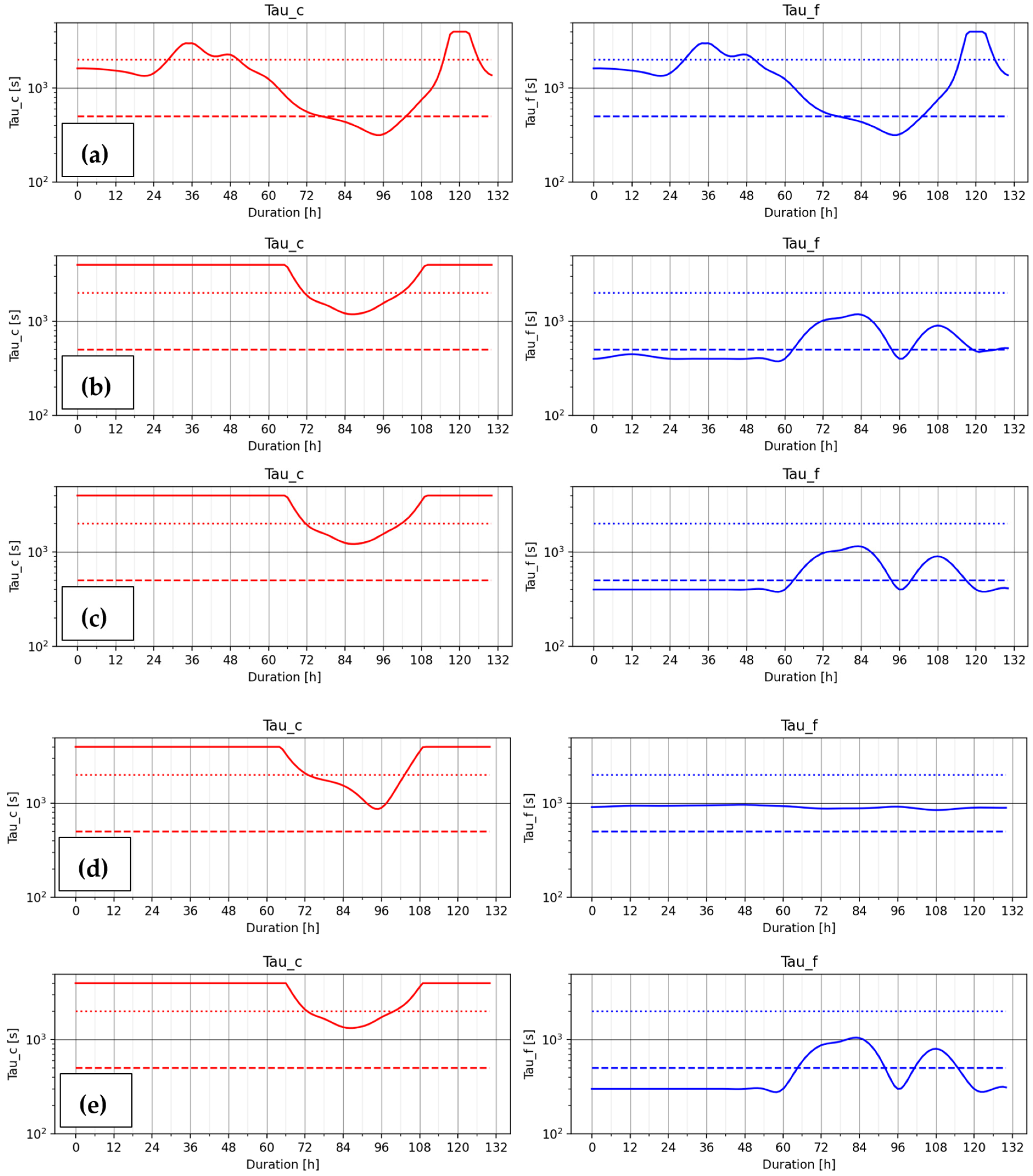
After the PE evaluation, the timescales for the conversion τc and fallout τf time-scales (expressed in s) were calculated. According to the formulae listed in Appendix B, five different options exist for tau computation, and Figure 12 shows their fluctuation during the event. Increasing the PE corresponds to a general decrease in τc (from 2000 to 3000 s to 500–1000 s) that was experienced in the central phase of the event (72–108 h). Conversely, the fallout terms exhibit less pronounced modification or a slight increase (from 500 s to 1000 s), except for the first graph, where the condition τc = τf is considered, so the two paths are the same. Looking at a sensitivity analysis, the τf variation from τf1 to τf4 is not dramatic, while the solution is quite different considering τf0, where τc = τf.
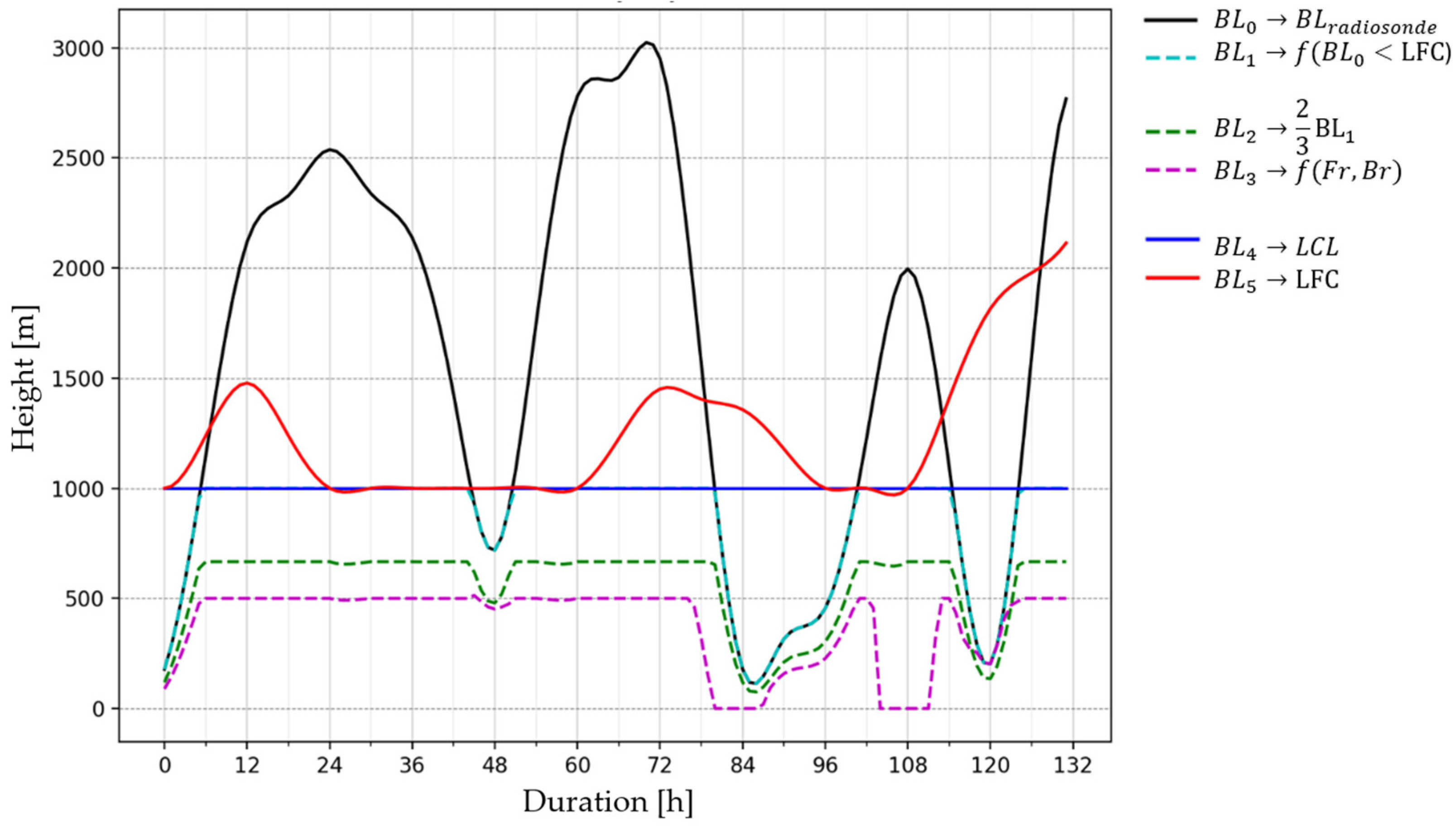
Another critical parameter is the boundary-layer elevation (BL). The former is rather difficult to evaluate explicitly due to its high spatial and temporal variability. According to the formulae listed in Appendix C, the BLi functions calculated from the Novara Cameri radiosonde data are represented in Figure 13. The fluctuation of BLi follows the day–night alternance with significant amplitude (from 0 up to 3000 m). However, the former should at least be corrected (i.e., decreased and remodulated) considering the wind flux dynamics at local and synoptic scales (see Appendix C). Including some of these corrections, six BLi functions have been reported, showing a significant reduction in the temporal variability around the mean value of 1000 m, typically recorded in the Po valley. Among them, the heights of BL3 and BL5 were retained as representative for defining a reasonable BL height range, where BL3 is the minimum (BL ≈ 500 m) while BL5 is the maximum (BL ≈ 1200 m). This range was tested within the sensitivity analysis, showing the importance and the influence of BL regarding the rainfall generation.

3.4. Global Error Analysis: Total Rainfall Fields Comparison

The 2D LUME model was tested considering four model routine combinations: warm–cold rain schemes with and without moist convection activated. As was reported in the case-study description, the event involved not only warm-rain precipitation, but significant amounts of snow (deriving from cold microphysics) were also extensively recorded. Moreover, the scirocco current plays the role of a humid southerly flow, carrying a large amount of water vapour and energy across the Piedmont area, which triggers sparse convective precipitation.
To appreciate the role played by ICs and BCs, a sensitivity analysis has been carried out using only the warm-rain scheme. In Table 5, the simulations that were carried out are listed, principally varying τi and BL configuration and evaluating the performances through the error metrics. The main outcomes of the sensitivity analysis on τi and BL are described here, looking at the total rainfall balance at the end of each simulation. Decreasing the BL height brings a non-negligible increase in precipitation. Generally speaking, BL can reduce the amount of “orographic updrafts”, since under the BL, the upslope flow can be considered not in motion, not contributing to the orographic process. However, evaluating BL as too high a value could be unrealistic, especially during a significant rainy event where the airflow dynamics and precipitation downdraft can mix all the atmospheric layers. An intermediate BL configuration (BL3 or BL5) has shown the best results, giving the lowest BIAS, RMSE, and SMAPE, and the highest values of CC. Among others, the lowest errors were reached for the simulation n°4 and n°6, where the BIAS, RMSE, SMAPE, and CC index were rather comparable, highlighting the negligible influence of τi change from 1 to 4 configuration. In both cases, the error analysis has suggested applying the “additive” error. In simulations n°4 and n°6, BL3 shows the lowest the BIAS errors, less than 4 mm on average (3.96 and 3.78 mm), and the lowest SMAPE (0.38 and 0.39), while CC displays the order of 0.92 >> 0.7. Looking at the cumulative errors (AIS statistic), both simulations n° 4 and 6 have shown the lowest values.
To explore the τi influence better, three control simulations, n°11, 12, and 13, have been conducted, testing the stationary condition of τf = τc assumed equal to 200 s (n°11), 500 s (n°12), and 2000 s (n°13). Increasing the microphysical time scales, the final rainfall field becomes much more dispersed, and the total amounts tend to decrease sensibly due to the spatial dispersion and the rainfall evaporation (increased by larger times of conversion and fallout). This is in accordance with the previous studies [23,26], confirming the critical role of τi in modulating the rainfall signal in the 2D domain as well. Statistical errors yield higher BIAS and RMSE with respect to the more realistic simulations, especially for lower values of τi, showing how the τi temporal dependence is better than the stationary option. Despite this, SMAPE (<0.5) and CC (>0.7) show that the rainfall field reconstructed is not so different from the real one.
The sensitivity analysis was extensively explored for the warm-rain case, while for the other three model configurations, only the BL layer influence, assuming τf = τf1 configuration, was evaluated. In Table 6, the best-score simulations conducted for the 4-model configuration are shown: warm and cold rain with and without convection activation. The error statistics have shown rather low BIAS errors (in the order of a few millimetres of rain), highlighting that the overall amount of precipitation is correctly reproduced: BIAS is less than 10 mm while RMSE is in the order of 100/20 mm for additive/multiplicative error models. Regarding the total field-cumulated rainfall, the model predicted the spatial rainfall pattern with CC ≥ 0.9 and SMAPE < 0.5 (in the order of 0.4) quite accurately. Moreover, RMSE is in the order of 100 mm, showing the significance of the spatial gradient in the precipitation results. AIS statistics have been recorded as higher for the convective case with respect to the non-convective case, ranking the cold scheme as the most representative.
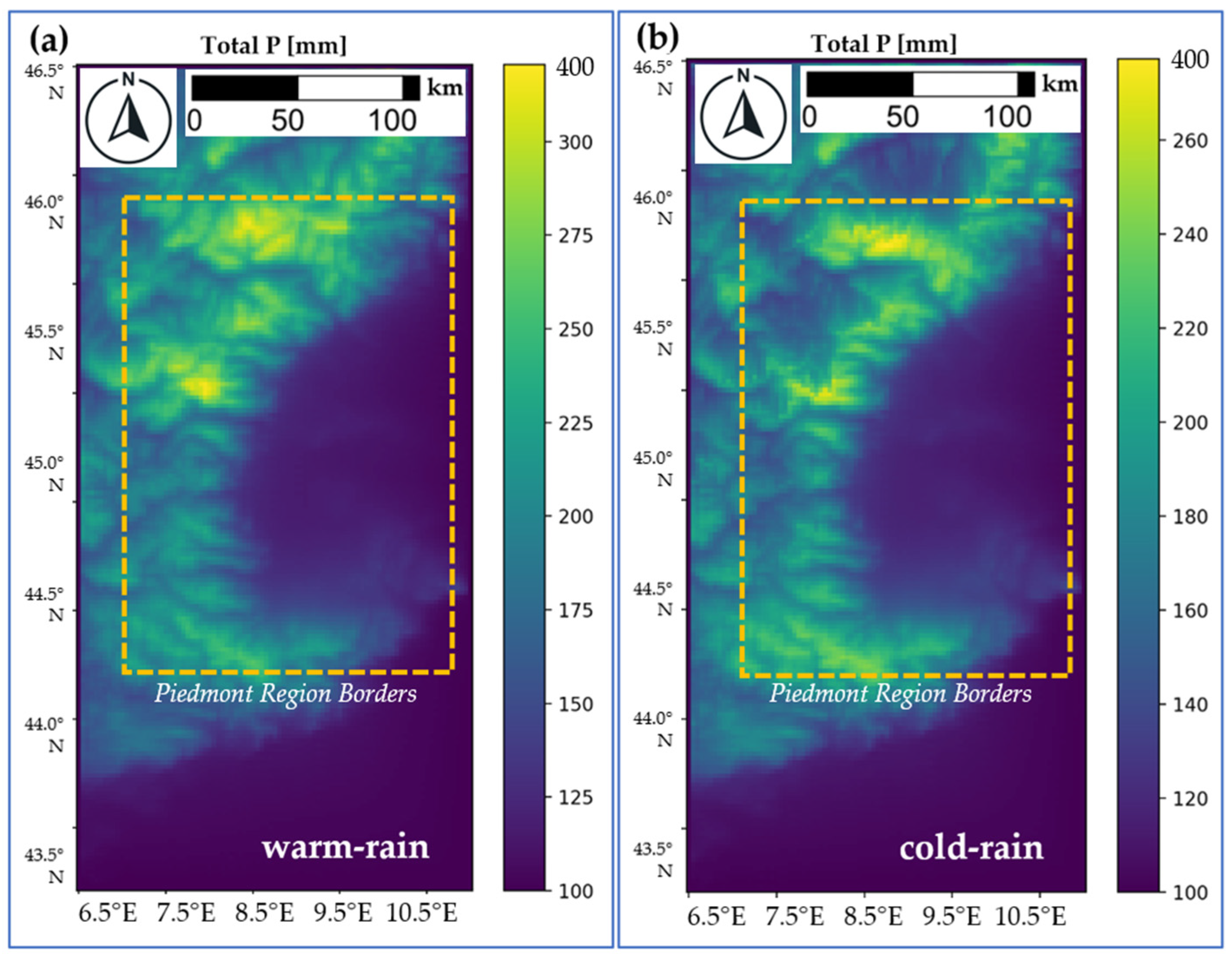
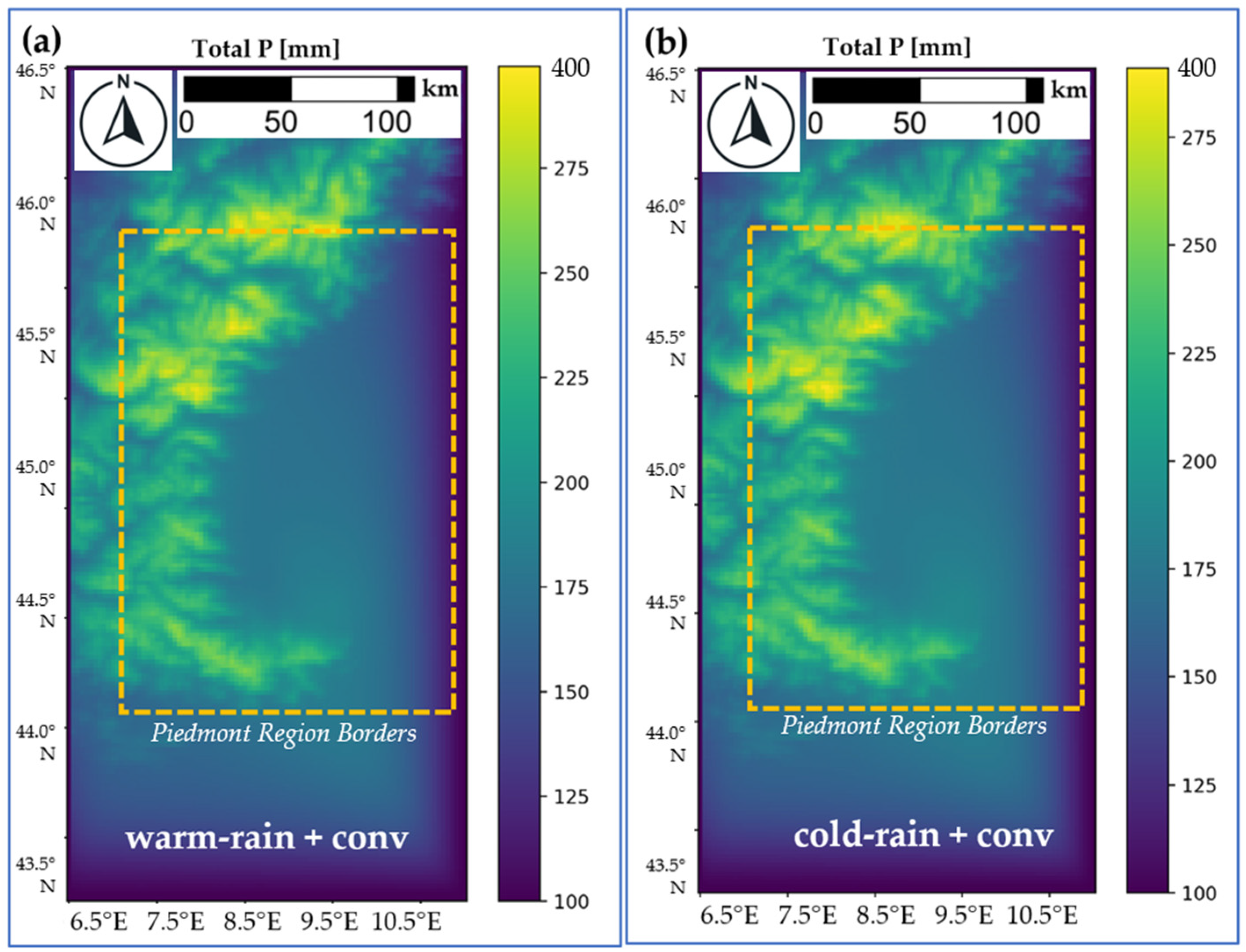
The error statistics evaluated in Table 6 are consolidated with the visual reproduction of the total rainfall field. From the ARPA Piemonte report [31], the total rainfall amount map has been extracted and compared with the simulation results. The latter generally agree in terms of spatial distribution and amounts (Figure 14 and Figure 15). The Alpine areas, corresponding to the Verbania and Biella provinces, have been detected as the ones with the maximum amount of precipitation. For the four microphysical routines, the model has simulated similar amounts of precipitation, reaching maximum values of up to 300–350 mm/event. The highest values were correctly simulated along the Alpine mountain ranges, while the lowest were localised across the floodplain. The peak values (recorded locally across the mountain range) are quite smooth and slightly underestimated (−20/30%), especially for the cold-rain scheme. Apart from this, the reconstruction qualitatively and quantitatively agrees with the reference maps provided by ARPA Piemonte [31].
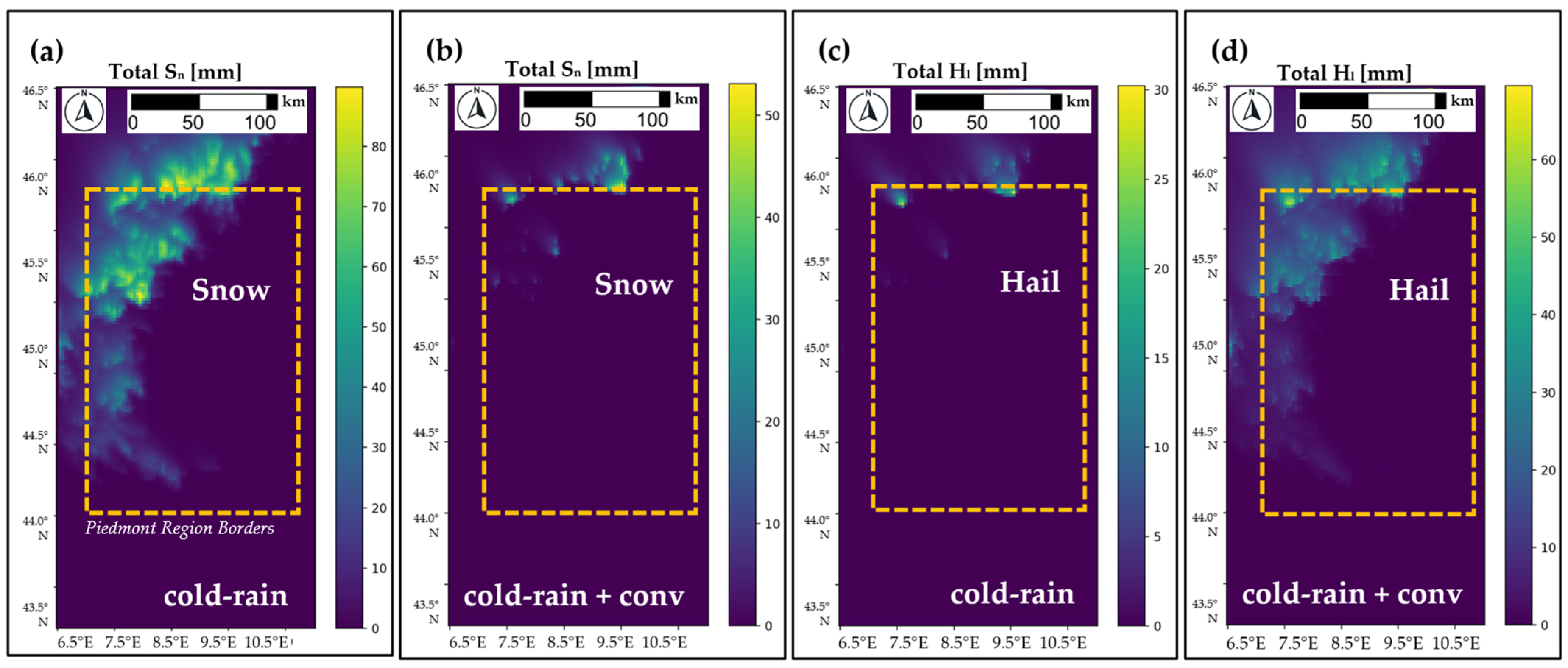
Even if the total amount of rainfall does not vary too much when changing the microphysical models, the type of precipitation simulated can change significantly. Applying the cold-rain scheme, rainfall may split into snow and hail, spreading across the Alpine area at the highest elevations (Figure 16). In particular, the amount now computed by the model has reached a maximum value of 100 mm, corresponding approximately to the 1 m of fresh snow recorded during the event by the local monitoring system [32]. Similar behaviour has been computed with lower amounts of hail and snow (up to 50–60 cm), with the cold scheme enabling the rainfall convection triggering. Hail and snow are dispersed across the northwestern part of the domain, showing that their formation has been triggered only across the highest mountain areas (>2000–2500 m). With respect to rain, this represents only a small portion and exhibits significant scattering across the domain. According to the type of microphysical model, the cold scheme calculated snow and hail formation within the investigated area and, adding the convective source, the total rainfall amounts have been slightly increased across the Po floodplain (up to +40%) while negligible variation has been simulated across the Alpine range. This result was expected, since increasing the local condensation sources due to moist convection enables higher latent heat to be released, considerably increasing the temperature in the surrounding areas with respect to the no-convection simulation. This is also responsible for the precipitation-type transition from snow to hail, which is more typical with convective environments.

3.5. Local Error Analysis: Single Rain-Gauge Comparison

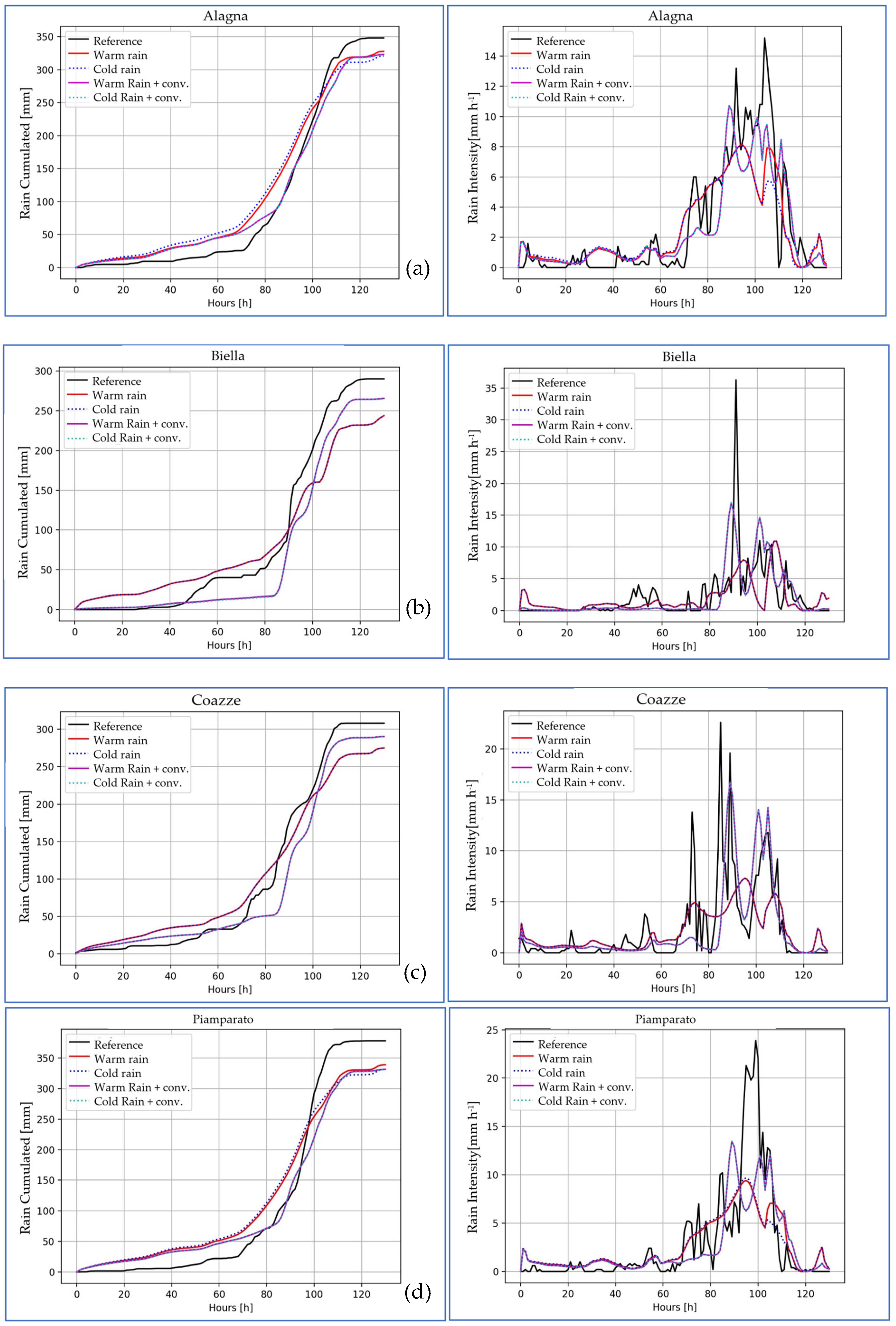
The global error analysis was extended locally by comparing model-predicted data series sampled at each rain-gauge location with respect to the corresponding measured series (reference). The comparison was carried out considering the cumulated rain (C) and the rainfall intensity (I) evolution through the simulated event (i.e., I(t) and C(t)) with respect to the microphysical routine adopted in the 2D LUME model. The comparison was carried out for all 56 reference rain gauges available in the region. Here, five stations, Alagna, Biella, Coazze, Piamparato, and Talucco (Figure 17), are shown. The five stations are located across the Piedmont Alpine range, and they have reproduced the investigated event well.
As was expected, the four microphysical schemes work differently locally:
Cumulated precipitation evolution generally follows the reference data, with “no-convection” routines slightly anticipating the “enabled-convection” versions. Moreover, the total amounts recorded at the end of the simulated event are comparable (with BIAS lower than 50 mm), confirming the results of the error analysis previously conducted.
The intensity pattern is rather interesting since the simulated rainfall is able to follow the reference data, giving a correct depiction of the rain rate pattern and highlighting the most intense phase of the event (between 15th and 17th of April). Again, “no-convection” models produce lower rain rates with respect to the “enabled-convection” routines. This is physically consistent, since convective rainfalls are reported to be most intense with respect to the stratiform ones. On the contrary, the high spikes recorded by reference rain-gauges are not always reproduced due to the numerical smoothing introduced by model time integration.
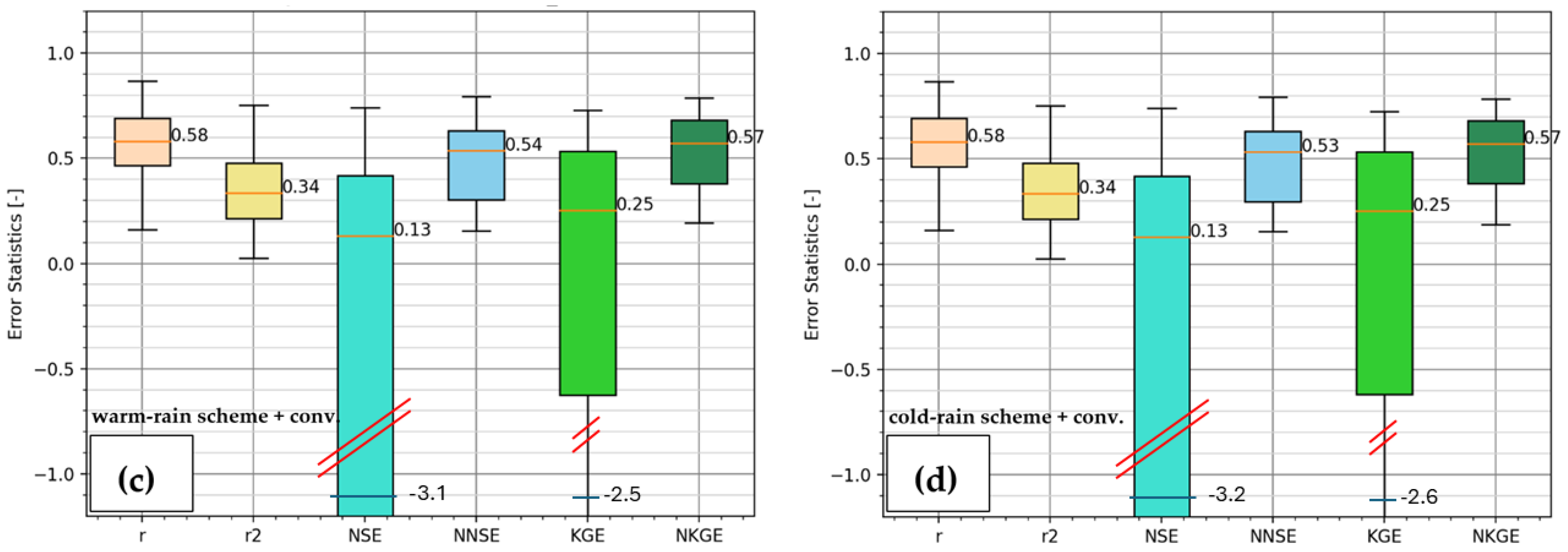
Local error analysis has been improved, considering all 56 stations. The error statistics investigated (Pearson correlation coefficients, NSE and KGE) are represented here in the form of a boxplot to highlight the variability of the rainfall sample, with respect to the four microphysical routines tested (Figure 18 and Figure 19). Cumulated rainfall (Figure 18) for the four cases exhibits high performance, evidencing that LUME 2D, independently form the type of model routines, is able to correctly reconstruct the rainfall cumulative evolution. Even if some indices (such as NSE and KGE) display significant dispersion, medians are located above 0.5, showing the effective prediction of the model. Pearson coefficients are very high (≈1), showing a quasi-perfect agreement (strong correlation) among the reference and simulated results. Conversely, as this was expected, the spatial and temporal variability in rainfall intensity reproduction is more significant (r ≈ 0.6 and r2 ≈ 0.35). Performances are settled above the 0 threshold (under which the model performance is insufficient) but are generally below 0.6, confirming the more casual pattern of the rainfall intensity signal. It can be noticed that, upon adding the convective term, the model performances may slightly degrade (lower median), increasing the overall solution variability and increasing the error statistic dispersion.

BIAS and NSE Evaluations Across the Investigated Area

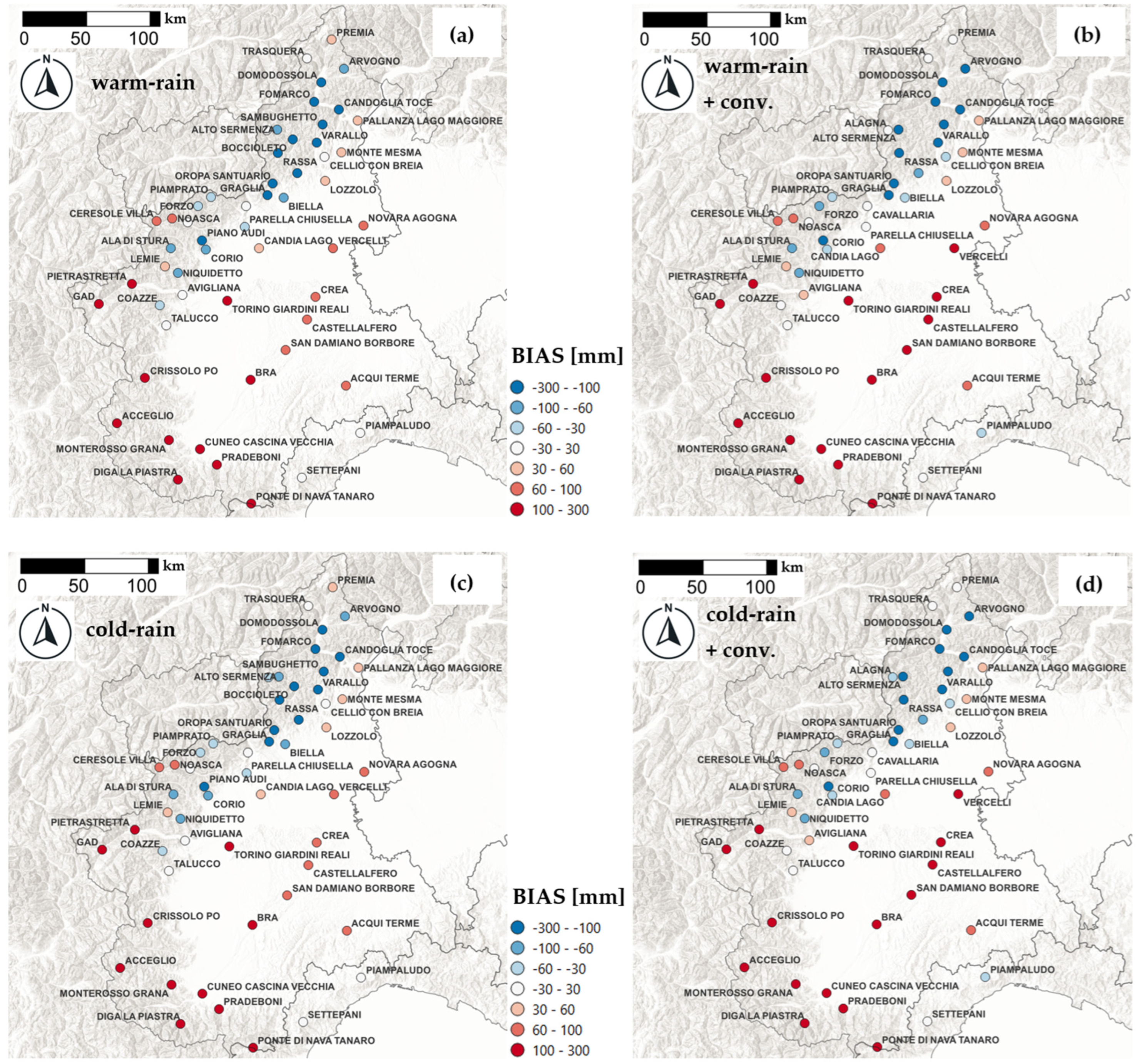
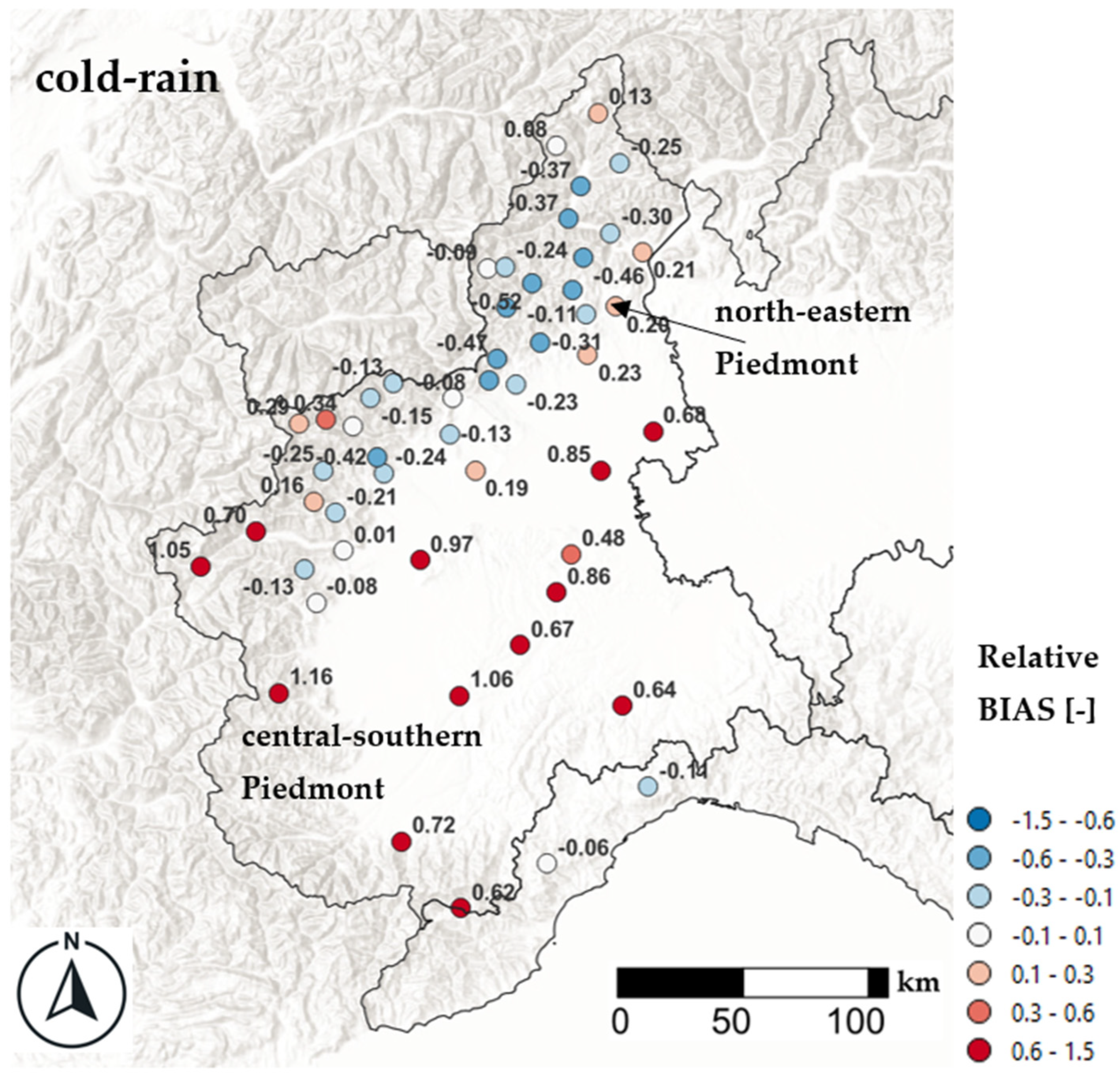
From the viewpoint of error analysis, knowing the area of the domain where the errors are higher/lower is useful to evaluate the skill of the model in predicting spatial rainfall distribution. Therefore, in the next three figures, Figure 20, Figure 21 and Figure 22, the BIAS and NSE indices have been depicted for each station across the region of Piedmont, showing their spatial distribution. As a confirmation of the previous analysis, the BIAS values recorded across the domain are not negligible and have a dipole polarisation: positive biases (i.e., model overestimation) are more consistent across the floodplain areas and are more pronounced for simulations where moist convection was enabled (Figure 20b,d); negative biases (i.e., model underestimations) are located across the Alps mountain range in the proximity of the highest rainfall amounts recorded in the northeastern part of Piedmont during the event. Here, the differences between convection-enabled and no-convection simulations are not remarkable. Among the four microphysical simulations, the “cold-rain” without moist convection activation has revealed itself to be the one with a lower number of overestimations > 100 mm across the floodplain (seven stations), while the number of mountain underestimations < −100 mm has been maintained between 10 and 15 stations for all the simulations. The underestimation of the highest peak was already addressed in the comparisons in Figure 17 (with a negative BIAS of around 50 mm). The latter trend was also confirmed by the BIAS calculated in Table 7, where the stations that exhibited the highest rainfall cumulates during the event (in Table 4) have been compared with LUME 2D results (considering the best simulation, n°2 of Table 6, where the snow, rain, and hail categories have been summed together). As can be observed, the BIASES are always negative and in the order of 100–150 mm, which represent almost 20–30% of the total precipitation amounts of these stations (between 450 and 650 mm). Even though the 20–30% could appear consistent, in reality, this represents a fairly good performance for meteorological models regarding the extreme rainfall peak estimations [3,8,25,26,27,60]. This comparison has shown how the model has been able to correctly reconstruct the largest amount of rain in that sector of the Piedmont region, which has been clearly enhanced by the orographic effect of the Alps range.
Biases can give just an overview of the differences between the simulated and the estimated total rainfall amounts at the end of the event. However, in the previous paragraph, some indices have been introduced to evaluate the accordance of simulated time-series of cumulated precipitation and intensities with reference data. These indices could be considered to establish the performance of LUME 2D across the Piedmont region. Among others, the NSE was adopted, with Figure 21 and Figure 22 showing the model behaviour with respect to the cumulated time-series and to the intensity time-series, both referring to the most intense phase of the investigated event, which occurred over ≈36–48 h between 15th and 17th of April 2025. As was already highlighted by the boxplots of Figure 18 and Figure 19, cumulated rainfall has higher performance skills with respect to the intensity. One aspect that determines this is that cumulated rainfall is a monotonically rising function that appears more or less steep depending on the amount of rainfall recorded at the station. Therefore, the effectiveness of the model appears rather high (NSE > 0.6), especially across the Alpine mountain range, confirming that those areas have experienced a better reconstruction of the rainfall distribution. Conversely, the floodplains are the areas where NSE drops under 0.2. Regarding the rainfall intensity, the LUME 2D scores are considerably lower, reaching values between 0.4 and 0.7 in the mountainous sector of northeastern Piedmont, while the values in the other places are generally lower than 0.2. These results were expected, since it is quite similar to the NSE performance depicted in the box plot, where median values in a range of 0.13–0.26 are characterised by significant dispersion. As a result, NSE analysis across the domain confirms that the LUME 2D model behaves better in the proximity of mountain ranges where the upslope mechanism triggered by orographic uplifts plays a major role in rainfall generation. However, across floodplains, where rainfall amounts are delivered by local convection or are the product of large-scale air-mass dynamics, the model is not able to glimpse them accurately.

4. Discussion

In this section, all the key points regarding LUME 2D tests are discussed.

4.1. A 2.5D Model Perspective

The 2D version of the LUME model was designed, taking into account the 3D complexities of the atmosphere [3]. With respect to the previous version, where the state of the atmosphere was retrieved from a single radiosonde profile, here the 2.5D perspective is introduced: more radiosondes are considered within the area of investigation, and more height layers are taken into account for computing atmospheric profiles and variables. With respect to a single-point vertical-integrated model, reconstructing a 2D-layered domain requires interpolation techniques to be included in the methodology [38]. However, even though the atmospheric state is precisely evaluated at the radiosonde location, their loose spatial distribution (≈200–300 km relative distances) and their coarse temporal frequency (12 h) should be considered. In this light, finding the best “spatial-temporal” interpolation technique is not a simple task, and since radiosonde data may significantly affect the rainfall simulations, it should be handled with care.
The temporal integration of radiosonde data is a challenging aspect, presented in Section 2.1.2 and Section 4.1. The mean diurnal evolution can be detected in principle, assuming that at 6:00 am and 6:00 pm the atmospheric state is intermediate, as it is between 00:00 am–12:00 pm and between 12:00 pm–00:00 am. This approximation is sufficiently accurate for “temporally smoother” variables such as T and RH, while it is not always true for more dynamic ones such as wind. In our case, to temporally interpolate the variables, the spline algorithm was adopted, since it was the one that admitted the lowest errors with respect to other types of interpolation techniques. Unfortunately, the abrupt variation between two radiosonde launches, such as the passing of a rapid cold front or squall lines, cannot be detected clearly. Another possibility to overcome these uncertainties would have been to consider GFS (Global Forecast System) outputs or other large-scale models’ outputs to complete the radiosonde data, increasing temporal coverage [61,62]. This “data mixing” would help to increase the accuracy of the BC and IC data, promoting the implementation of LUME 2D not only for reanalysis but also for rainfall nowcasting. This solution is now under study, also considering the global model data accessibility.
To avoid increasing the computational cost, the domain extension adopted for LUME 2D was generally tailored to the investigated area, which is an advantage, but it may not encompass more than one or two radiosonde stations (in the case of Piedmont, radiosondes of Novara-Cameri and Cuneo were involved). When using only two stations, the spatial interpolation procedure generally fails (only the nearest neighbour of the inverse-distance-weight algorithm may work, while the spline or complex algorithms are not applicable), and the horizontal advection and the synoptic-scale variability could be poorly represented (or not reproduced at all). Therefore, the enlarged domain introduced in this study was designed to increase the number of radiosonde stations in the surroundings of the investigated area, potentially sharpening the accuracy of the spatial interpolation of atmospheric variables (in the enlarged domain, nine radiosonde stations were analysed). As a result, especially for wind variables, their field reconstruction was revealed to be more accurate, both in the upslope regions (Southern Alps) and across the downslope flanks (Northern Alps).
As can be observed, initial data preparation represents the most time-consuming part of the LUME 2D implementation. Fortunately, the available algorithms and methodologies for 2D field reconstruction are many [38,63]. Here, the spline algorithm has been applied, since these interpolation curves were able to reconstruct, in space and time, the highly variable atmospheric fields, sometimes characterised by steep gradients [38,40]. Splines have been reported to be quite sensitive to the spatial distribution of the reference points. So, a double-step interpolation method (nearest-neighbour + spline) has been implemented in order to ensure the most accurate 2D reconstruction. Bearing in mind the possible limitations embedded in radiosonde data, this interpolation technique has performed well (admitting negligible errors), especially when describing wind magnitude, wind direction, and convective index fields. [6]. Wind updrafts and convective parameters are crucial for convective activation, so this approach extended the evaluation of the triggering functions over a 2D domain.
The 2.5D perspective permits simplifying the “nesting” operation, allowing the user to easily set the boundary conditions (BCs). In the previous 1D version, LUME required only the initial conditions at x = 0 of the trace [23], but now, since the domain is 2D, the square BCs are necessary. The enlarged domain has helped in this sense, giving the user a set of BCs (in a tractable file format .netcdf) to employ and synchronise in the computational domain. In this regard, the reconstructed wind fields of velocity and direction were delivered to LUME 2D to specify the BCs at the computational domain borders for each timestep, taking into account the variability driven by large-scale dynamics. Moreover, the convective index fields were taken into account to feed the moist convection triggering functions. BCs nesting procedure was herein described in a user-friendly way, bearing in mind that it represents one of the most delicate tasks for local area meteorological models (LAM) initialisation [64,65]. In the LUME 2D code, the user is allowed to set and customise the proper BC simulations, passing from enlarged domain analysis to the investigated area. Altering “nesting” allows the user to see how sensitive the model could be to BCs and how the results may be perturbed by different settings, raising awareness about the initial data accuracy.

4.2. Sensitivity Analysis on Microphysical Parameters

The 2.5D approach has improved the reconstruction of the BCs and ICs for the LUME 2D model, but uncertainties about rainfall parameterisation remain due to the non-linear microphysical processes. Therefore, the sensitivity analysis has assessed the influence of PE, τi, and BL, already highlighted, in the precedent 1D version of the model, as the most critical parameters for rainfall generation.
Precipitation efficiency is a proxy parameter which can be retrieved empirically from radiosonde data. Why is it so important? Several authors [22,66,67,68,69] have tried to explain it, proposing different formulations to measure the efficiency of the microphysical process in the conversion of water vapour into rainfall. From a geo-hydrological viewpoint, few variations in the PE may lead to a transition from a no-rain scenario to catastrophic flash floods [15]. This could be exacerbated across mountain ranges where the orographic action may dramatically enhance the PE, increasing the amount of water vapour condensed in clouds. PE enhancement within the Alps and Apennines ranges due to strong and blocked orographic upslope effects is one of the causes of the critical geo-hydrological episodes recorded in the past [20]. Therefore, trying to find a method to predict this parameter just by looking at radiosonde data and the index represents a goal that was pursued in this work, proposing different formulae of PE. Due to the significant importance of this quantity, further investigations were carried out using Artificial Intelligence algorithms [41] in order to enhance the prediction of the general trend, taking into account its significant temporal and spatial variation. As can be observed from the GLM regression, PE depends not only on local data (i.e., PW) but also on global (synoptic) variables (i.e., WS) that are related to the flow motion conditions [26]. The latter may be difficult to disentangle during a complex and chaotic rainfall event. In this sense, PE general behaviour should be described in the following way: a general trend (synoptically driven) + a variability (locally driven) [68]. As a matter of fact, the PE has been interpreted as a statistical quantity characterised by its own distribution, mean, and variance.
According to [26,29], the PE parameter is a measure of how fast the microphysical processes are. They have proposed some analytical equations to estimate PE from τi, but, as was applied in the previous LUME version, these equations have been reversed in order to estimate τi from PE. Since τi time scales are also included in warm and cold schemes of COSMO for measuring the rapidity of microphysical processes, five parameterisations of τi have been proposed in the study (see Appendix B). Again, since they depend on PE estimation, their value could be uncertain and may fall outside the “canonical” ranges of 200–2000 s [26]. Moreover, τi coefficients are not constant in time, since the microphysical processes may accelerate and decelerate under certain conditions [30] (that could be related to the presence of moist convection activation). In the 2D LUME model, the sensitivity analysis has shown a slight variability in the τi solution depending on the parameterisation of τf, which does not affect the final rainfall reconstruction dramatically. On the other hand, the simple condition τc = τf is very different from the other ones. From a microphysical viewpoint, it is also the least frequent situation since (in general) τc and τf are comparable but not necessarily identical since they describe two different processes (conversion and fallout).
Three key “synthetic simulations” have been carried out to show the effect of τc and τf magnitude. Decreasing the τi values, the computed rainfall field appears less spatially diffused and more clustered in the proximity of the steepest upslopes. In Figure 23, the differences among the three “synthetic simulations” are reported. Increasing τi values, total rainfall becomes more diffused across the domain, significantly reducing the peak amount of total rainfall (from >800 mm for 200 s up to ≈ 300 mm for 2000 s). Short time scales have a strong influence on the total amounts but may last only for a certain period, and usually they do not dominate the entire event [70]. This fact is confirmed by error statistics like BIAS and the SMAPE index, which reduce from ≈150 mm to ≈10 mm and from 0.5 to 0.4, respectively, showing a better rainfall reconstruction when applying a long timescale. In reality, τc and τf vary in time and space, leading to a combination of the short and long timescales. Up until now, τc and τf have been specified as a unique value across the computation domain (considering the most representative radiosonde station), but their spatial distribution is under study, also taking into account the possible influence of the other atmospheric variables and ridge velocity.
The formulation of τi follows an analytical expression which depends on the “geometry” of the mountain range (see Appendix B). According to [26], it could be associated with a “ridge” or “sinusoidal” type. If a ridge is selected, the mountain range is interpreted as a unique ridge characterised by a certain width and height; conversely, with a sinusoidal mountain range, a periodic ridge with a certain width (wavelength) and height (amplitude) is applied. Even though the two expressions are quite similar, the results may evolve in a completely different way since the key parameters of the microphysical process are strongly perturbed. The simulation conducted with LUME 2D has considered the single ridge option in accordance with other similar studies conducted across the Alps. In the sensitivity analysis carried out with the warm-rain routine, the behaviour of the model was investigated, showing unrealistic total rainfall amounts (+50–60%, 350–400 mm simulated against ≈250 mm recorded). These simulations were discarded for the Alpine range, but the sinusoidal option could be applied over areas with shallower and regular mountain ranges where the sinusoidal behaviour of the airflow could be much more representative [26].
As reported in [23], BL is a quantity extremely difficult to estimate since it is strongly perturbed by local factors (temperature and buoyancy) and has a great temporal and spatial variability [71]. Nonetheless, an upslope model is able to modulate the rainfall amounts, controlling the intensity of the orographic upslope mechanism. High BL reduces the upslope areas, so the conversion of water vapours into condensed ones and vice versa. The latter is directly appreciated in sensitivity analysis, comparing the simulations n°4–5 and 9–10: knowing that BL3 < BL5, the mean total rainfall has decreased from 259 to 228 mm and 361 to 280 mm, reducing by about 10–20%. However, the mechanisms involving BL with precipitation are more complex, and they have not been included in this work. This simple solution, which was already described in the 1D version, has been reincluded in the 2D version, improving the BL estimation as a function of time (see Appendix C). Like the PE, BL has also been interpreted as a statistical quantity characterised by its own distribution, mean, and variance. BL is therefore one of the principal calibration parameters that, in this study, was adjusted in order to improve the model performance after the sensitivity analysis. Developments on BL estimation represent an active research frontier, and advances are planned to be included in the further code may include an explicit BL evolution model.

4.3. Cold-Rain Dynamics

One of the novelties proposed in the LUME 2D model is the inclusion of the microphysical schemes of precipitation. The latter were not considered in the previous version of the model in order to keep the rainfall-generation processes as simple as possible. According to [30], the cold-rain scheme represents an extension of the warm-rain scheme where two additional microphysical categories have been included (i.e., snow and hail). Why are those categories needed? The warm-rain scheme is able only to compute warm-rain microphysical processes (such as nucleation and accretion), which occur in a warm cloud [36]. Unfortunately, warm-rain processes are neither the most common nor the most frequent in a cloud [30], where cold-microphysics generally play a major role. Therefore, cold schemes can better represent the evolution of the rainfall process but need to be parametrised (so their computational cost is higher). Cold schemes can produce snow and hail that generally coexist with rain in the winter and summer periods, respectively.
On certain occasions, snow accumulation can be a consistent part of the total rain accumulation, as the case study investigated in this work. Computed snowfall amounts have reached values up to 80–100 cm across the Alpine areas, in agreement with recorded reference data. From a geo-hydrological viewpoint, the presence of snow is significant since it can decrease the total amount of rainfall effectively discharged in the river network after a heavy rainfall episode [72,73]. This is not a secondary aspect: water that falls as snow is stored in the basin and released after some time when melting occurs, contributing to delaying the peak discharge. Snow can also be stored as a water resource, so that the cold-rain scheme could be helpful in reconstructing basin hydrological balances. Conversely, during the summer period, hail is an index of where moist convection has occurred in a certain region [3,5]. Cold scheme is able to spot these peculiarities of the event, showing the areas that have probably also experienced the highest rainfall rates (hail formation is related to strong updrafts). Hail is also associated with object damage (cars, windows), physical injuries, and sewage clogging, so knowing the locations in which hail is possible is undoubtedly useful to prevent these types of issues [74].
In this case study, the cold scheme was the one with the lowest errors (BIAS and RMSE) and the one that resulted in the most convincing reconstruction of rainfall–snow–hail fields. Snow accounted for ≈20–30% of the total rainfall, while the hail, even though it was reported in the chronicles, accounted for a rather small portion, less than 5% (Figure 16). The latter is compatible with the weak and rather scattered moist convection that was triggered on that occasion [31,32]. The cold scheme was relatively simple to implement since it was derived from the warm scheme with the simple inclusion of two more equations in the system. Only the snow and hail microphysical timescales have been parameterised, deriving their function from rainfall timescales τi, and enlarging (2×) and reducing (0.5×) their amounts, respectively. These may appear as a rough approximation, since they do not explicitly take into account all the waterdrop transformations (melting and freezing) [30]; however, looking at the model results, their simple formulation has been shown to be quite effective. The next step of the model will try to include the ice scheme. The former is the most complete microphysical scheme (but also the most complicated, since ice transformations are characterised by high non-linearities) that includes ice (i.e., qi) as a new category [30,33].

4.4. Moist Convection Contribution to Extreme Precipitation

Moist convection is the third new feature introduced in LUME 2D. The aim was to transform a purely upslope model into a more complete one, stemming from the need to study heavy-precipitation events that often occur due to moist convection triggering [4,15]. Here, moist convection was introduced using the superimposition principle to maintain the linearity of the model equations. It is interpreted as an additional source of condensed water vapour characterised by two main elements: the triggering functions and the magnitude.
Triggering functions have been retrieved from an extensive survey of the literature, pointing out the attention placed on simple threshold equations or procedures to be easily implemented within the LUME 2D routine. Each threshold defines a necessary but not sufficient condition for moist convection, so uncertainties about its fine-tuning are well known in the literature [3,49]. To overcome this problem, several authors [3,24,49] have proposed a combination of atmospheric parameters (such as temperature and humidity) with convective indexes retrieved from radiosonde data. Other authors [75] have applied this approach, especially for analysing large domains of long data series (such as climatic models), retrieving particular trends of the moist convection under a changing climate. Even though this method is useful for defining the threshold’s value, trying to combine them requires normalisation, since each function has its own scale. In LUME 2D, these functions have been normalised between 0 and 1 with respect to their value range and combined for evaluating the probability of convection. This probability has a key role and is fundamental to modulating in space and in time the expected amount of convective rain. Therefore, constructing an ensemble of convective triggering functions is an innovative way to introduce a statistical interpretation of the moist convection activation, increasing the flexibility of the threshold-based approach without losing its generality. Pconv can reduce the errors associated with the use of a singular formula and takes into account all the possible influencing variables on this non-linear process embedded within the index calculation.
The magnitude of moisture convection, i.e., the rainfall intensity of the thunderstorm triggered, cannot be explicitly resolved within a domain without a careful description of the mass and energy balances [6,76]. This is a critical point of the LAM model, which sometimes needs to be heavily parameterised for moisture convection, resolving it implicitly with bulk-scheme models [77,78]. The proposed G function for evaluating the magnitude was applied for retrieving representative rainfall rates. These rates are expressed as rainfall intensities but cannot be directly measured since they are derived from a one-dimensional convective cloud model proposed by Kessler. G is therefore an empirical source for condensed vapour in LUME 2D that, even though designed for 1D models, has been applied across a 2D domain. The G function is not the only one in the literature; several authors [34,52,79] have tried to compute potential rainfall rates triggered by convection. These formulas may be more precise in estimating the convection magnitude, but require careful application. They depend on several atmospheric parameters rather variable in space and time, and are related to the latent heat-release mechanism. Conversely, the G function has a simpler equation, depending solely on the estimated updraft and convective heights, which normally exhibit a well-known range of possible values [3]. As a result, the G function could be easily tuned during the calibration phases of LUME 2D.
As noted from the simulations conducted, the convection is activated too broadly across the domain, not reproducing the bubbling/scattering effects typical of the convective processes (Figure 15). Furthermore, the typical convective rain bands [80], which are very frequent across mountain landscapes, are not reproduced at all. This happens since the moist convection development–dissipation cycle is not explicitly described in LUME 2D. Primarily, the spatial (≤10 km) and temporal (≈1 h) resolution of convective processes has scales lower or at least comparable to LUME 2D numerical integration (fixed at 2 km and 1 h). This zone (called “grey zone”) refers to a range of grid (1–10 km) and temporal (≈1 h) resolutions where neither a bulk nor an explicit representation of convection is ideal [5]. This issue is common in the LAMs where bulk–convective routines are applied [78], approximating the effects of convection on a larger scale, including updrafts, downdrafts, and cloud formation [24]. Unfortunately, the errors introduced by traditional parameterisations may become more significant increasing to sharp the grid resolutions. On the other hand, Convection-Resolving Models (CRMs) attempt to explicitly simulate deep convection, using high-resolution grids (typically around 1–4 km) to simulate the physical processes. CRMs face challenges with computational costs (requiring a larger number of atmosphere layers) and the need for high-resolution simulations, since the size and properties of simulated convective cells can be sensitive to grid spacing [51]. Therefore, within the “grey zone” where a mix of both approaches is requested [6], scale-aware schemes may be needed [24] since they are being developed to adjust their behaviour based on the grid spacing. In LUME 2D, moist convection is neither resolved explicitly nor described through a bulk model, but is simply parameterised. Therefore, further developments will go in this direction, trying to better integrate moist convection within the code using the convective approaches cited [30].

4.5. Non-Orographic Areas and Pbase Estimation

In this work, an extensive error analysis has been conducted in order to better assess the performance of LUME 2D. Several error statistics have been calculated and two different error models have been applied to study the accordance between simulated and reference time-series under different parameter settings of the model. Even though the global performance has achieved good scores when looking at the entire computational domain scale (BIAS and RMSE were generally low, see Table 5) and a near-realistic rainfall distribution has been reached (SMAPE < 0.5 and CC ≈ 0.9), moving to the local scale, the variability and the complexity of reconstructing a representative rainfall signal are evident. In fact, moving through the computational domain and considering the four simulations conducted applying different microphysical models (Table 6), the rain-gauge errors have shown a rather interesting “polarised dipole” distribution. Looking at Figure 20, Figure 21 and Figure 22, across the domain, the mountain areas located in the northeastern part of Piedmont are the ones where the model results exhibited the best accordance with the reference data. Across this region, both BIAS and NSE have shown the best scores (lowest BIAS and higher NSE), confirming the ability of LUME 2D in interpreting heavy orographically induced rainfalls. Even though a BIAS underestimation of 100 mm has been detected, it corresponds to a relative difference with respect to the reference of about 20–30% which is in the order of the expected error for this type of model [23,29,71,81] (see Figure 24).
On the contrary, the worst behaviour of the model was recorded across floodplain areas where no orographic uplift mechanism was experienced by the incoming airflow. This aspect is a known issue of the orographic upslope models, already addressed by [27,28]. The upslope model’s inability to compute the possible precipitation coming from synoptic air-mass dynamics and induced by warm- and cold-front passage across a flat area represents a strong limitation for the application of LUME 2D as well. In the simulation conducted for the investigated event, a spatially uniform Pbase of 100 mm of rain has been added to the rain field computed. This value was established from the analysis of rainfall records for the station located across the floodplain area of central Piedmont. Adding Pbase to LUME 2D results has been revealed not to be a good strategy, reducing the biases across mountain ranges but leading to an anomalous overestimation of the rainfall amounts across floodplains, especially for the cases where moist convection was activated (as can be observed in Figure 20). Moreover, during the event of April 2025, the Piedmont southwestern floodplain area experienced a so-called “pluviometric shadow” [31,32]. The pluviometric shadow of Piedmont is a consequence of the region’s surrounding mountains, particularly the Alps, which block moist air, creating a drier, “shadowed” area in the plains, such as around Cuneo (central–southern Piedmont), that receives less rainfall than the mountainous windward sides. This orographic effect reduces moisture on the leeward side of the mountains, leading to drier conditions. These effects, which are related to the interaction between large-scale air masses and the local orography, are not explicitly taken into account by LUME 2D. Therefore, this aspect has probably exacerbated the differences among simulated and the effective rainfall distribution, contributing to increases in the LUME 2D overestimation of P across central and southern–western areas of Piedmont. The uncertainties related to Pbase estimation and correction are under investigation and will be fixed in future updates with the aim of increasing the performance of the model across non-orographic areas as well.

4.6. Practical Indication for Model Implementation

In this final section, some practical indications for using LUME 2D in the most efficient way are described. They are intended to better clarify what has already been discussed in the previous paragraphs from the point of view of the model user. Among others, some topics are elaborated upon:
The choice of ICs and BCs in function of WVF;
The reanalysis and forecast modes;
The effect of DEM resolution;
The spatial extension of the computational domain.
The horizontal advection and the synoptic-scale variability are perturbed mainly by the wind dynamics, which can significantly change the magnitude and the direction of the WVF vector. Here, the wind variability is generally more pronounced than thermodynamics (i.e., PW, a function of T and RH, and atmospheric density), so that a better reconstruction of the wind velocity and direction fields is necessary to increase the accuracy of BCs and ICs provided to the computation domain. A wrong estimation of WVF magnitude or direction can lead to a completely different rainfall scenario, inverting the upslope processes (i.e., condensation of qv) into downslope dissipation (i.e., evaporation of qv) and misrepresenting the total rainfall field. Due to the high variability of WVF, the model cannot self-generate it (the computational domain is too small). WVF is the driving force of the model, as specified in Equations (5) and (34). Taking radiosonde data as the “sources” for calculating the evolution in time of WVF, the model simply propagates in space and time through the computational domain, describing its interaction with orography. Therefore, to drive the model, BCs (i.e., WVF fluctuation in space and time) need to be constantly provided at the border of the domain (in space and time) covering the entire duration of the event. Generally speaking, the rainfall event starts when WVF > 200–400 kg m−1 s−1 and finishes when WVF < 200–400 kg m−1 s−1, as clearly depicted by Figure 6. In the case study presented, BCs (at the border of the computational domain, nested from the enlarged domain) are updated on an hourly basis (see Figure 5c) while the model integrates the microphysical equation with a sub-hourly timestep, satisfying the CFL stability conditions. All the output data (i.e., rain, etc.) are reported at the end of each hour and saved in .netcdf file format.
LUME 2D can work in two ways, depending on the interests of the analysis. In the case study presented, a reanalysis (or back-analysis) was performed using recorded radiosonde data to generate interpolated spatial fields for ICs and BCs required. In the case of forecasting, the model can work similarly, but the BCs need to be provided by large area forecast models (such as the GFS model). In this case, LUME 2D can refine the large-scale forecast, highlighting with further accuracy the interaction between the WVF, the orography, and other local-area features (that in a large model may be coarsely represented).
The effect of DEM resolution on total rainfall amounts has already been examined in the previous works of LUME, where the 1D version of the code has been implemented [8,23]. There, DEMs with resolutions between 500, 1000, 2000, and 5000 m have been tested, showing that decreasing the resolution can increase the smoothing of the precipitation field. This is related to the upslope–downslope term of water-cloud generation (i.e., Cw in Equation (2)) that is in function of the calculated DEM slope. Namely, with higher resolution, DEM local slopes may eventually exhibit higher gradients, while, conversely, coarse resolution lead to a smoother representation of the DEM gradients. In this paper, this sensitivity analysis was not reported, but we decided to consider a DEM resolution within the “grey zone” (i.e., comprised between 1000 m and 10,000 m). A trade-off between the better DEM resolution and excluding moist convection explicit description has been found for the range of 1000–5000 m, so 2000 m was retained as a good compromise. Moreover, attention was paid to computational times, which were reasonably maintained (1 h simulated in 1 or 2 s) considering the resolution.
The model has been applied at a regional scale (Piedmont region) since the aim of the analysis was to test it on a rainfall event that hit the western sector of the Alps (≈100,000 km2). The model can work at any range (all the Alpine range could be analysed, for example), but more careful attention should be paid to the definitions of ICs and BCs. In fact, enlarging the extension of the computational domain may lead to a wrong interpretation of the state of the atmosphere in the areas far from BC conditioning. Even though the LUME 2D includes the microphysics of the precipitation, all the BL processes and sea-atmosphere and terrain-atmosphere feedback that may occur in the troposphere are not explicitly taken into account, leading to an incomplete reconstruction of the atmospheric state. In Table 8, the main practical indications for the model implementation discussed in this paragraph are presented.

4.7. Open Issues and Further Developments

In the previous paragraphs, a series of unresolved problems regarding the new LUME 2D have been discussed and are summarised below:
BC uncertainties and domain nesting;
Radiosonde parameter inaccuracies and variabilities;
Cold-rain microphysical schemes and their parametrisation;
Moist convection activation in space and time and its magnitude;
Pbase evaluation across non-orographic areas.
Even if they have been presented as a novelty, they will stimulate further developments in order to make the code complete and more versatile. The domain-nesting procedure is planned to be fully automated, improving the accuracy in the estimation of BC and IC testing as well as other interpolation algorithms. PE, BL, and other model parameters will be revised, trying to improve their empirical estimation from radiosonde data, explicitly considering their spatial dependence, and giving a more statistical interpretation of their representative values. The COSMO ice scheme, which is one of the more complete microphysical schemes, will be included in LUME 2D and tested. Moreover, moist convection will be improved, including energy balance-derived equations (such as CAPE closure [30,82]), new triggering functions, and magnitude estimation, taking into consideration the most appropriate approach for convective parameterisation. These further steps will contribute to refining the model solutions, improving its versatility, and enlarging its field of application. Since the precipitation types (rain, snow, and hail) represent the LUME 2D main outputs, a coupling with a geo-hydrological model could make for an interesting model chain for better studying critical heavy rainfall events.

5. Conclusions

In this work, an evolution of the LUME (Linear Upslope Model Experiment), designed to simplify the study of the rainfall process, was presented. The main novelties of the LUME 2D version regard (1) the 2D domain extension, (2) the inclusion of warm-rain and cold-rain bulk-microphysical schemes (including snow and hail categories), and (3) the simulation of moist convection activation.
The model was tested on a heavy rainfall event that occurred in Piedmont in April 2025. Using a 2D spatial and temporal interpolation of the radiosonde data, the model was able to reconstruct the 2.5D state of the atmosphere before, during, and after the analysed event. Then, the interpolated data were nested within the model domain through the specification of BCs and ICs, while the warm-rain scheme was selected for carrying out a brief sensitivity analysis on parameterisation. The cold microphysics scheme evaluated the snow and hail amounts, while the rainfall intensity amplification due to moist convection activation was detected in the results. The analysis of the rainfall fields simulated by LUME 2D has been evaluated against the reference rain gauges using two different strategies (global and local). Several error statistics were proposed for measuring the agreement of the simulations to the references (varying BCs, ICs, and microphysical routines), showing the fairly good performance of the model. The cold scheme without convection activation has performed best, while the moist convection activation has slightly improved the rainfall intensity scores, amplifying rain rates across the floodplain.
The goal of the work was to illustrate the LUME 2D main functionalities as clearly as possible. As a matter of fact, moist convection requires a certain grade of accuracy and embeds a measure of aleatory in the process. Trying to deal with these uncertainties and keeping the LUME 2D mathematics simple is not easy, but it is worth it. Bearing in mind that the results are encouraging (the model is numerically stable, and the rainfall rates produced and their spatial distribution are reasonable), further improvements are required to increase the spatial prediction of the localised convective storm, including non-linear terms and energy balance equations. Moreover, regarding the aspects that should be handled with care during LUME 2D calibration (such as BL and microphysics timescale parameterisation), its capabilities will be improved in the future version of the code.
Rainfall is the result of complex microphysical processes that happen within a cloud. Having a tool able to reconstruct rainfall processes easily and understandably, when compared to the more complex LAM, is advisable for non-expert stakeholders and researchers operating in rainfall management fields and those interested in preventing and controlling the possible consequences of rainfall-induced geo-hydrological issues.

Author Contributions

Conceptualization, A.A. and F.A.; methodology, A.A.; software, A.A.; validation, A.A. and F.A.; formal analysis, A.A.; investigation, A.A.; resources, A.A.; data curation, A.A.; writing—original draft preparation, A.A.; writing—review and editing, A.A.; visualisation, A.A.; supervision, A.A. and F.A. All authors have read and agreed to the published version of the manuscript.

Funding

This work has been financed by the Research Fund for the Italian Electrical System under the Three-Year Research Plan 2025–2027 (MASE, Decree n.388 of 6 November 2024), in compliance with the Decree of 12 April 2024.

Institutional Review Board Statement

Not applicable.

Informed Consent Statement

Not applicable.

Data Availability Statement

The model presented in this study and its Python code are available from the authors on request. The other data (such as radiosonde and rainfall data) were derived from the following resources available in the public domain: University of Wyoming Atmospheric Science Radiosonde Archive and Richieste dati|Arpa Piemonte.

Conflicts of Interest

Authors Andrea Abbate and Francesco Apadula were employed by the company RSE S.p.A—Ricerca Sistema Energetico.

Abbreviations

The following abbreviations are used in this manuscript:
LUMELinear Upslope Model Extension
RMSERoot Mean Square Error
AISAll Indicator Scores
SMAPESymmetric Mean Absolute Percentage Error
CCCorrelation Coefficient
NSENash–Sutcliffe Efficiency
KGEKling–Gupta Efficiency
PEPrecipitation Efficiency
BLBoundary Layer
ELEquilibrium Layer
LFCLayer of Free Convection
LCLLifting Condensation Level
GLMGeneral Linear Model
CRMCloud Resolving Models
LAMLocal Area Model

Appendix A

In Appendix A, all the equations adopted for the PE (precipitation efficiency) prediction evaluated from radiosonde data are listed. In particular:
PENoel [66] is a formulation that simply correlates PE with the PW and RH parameters (A5). It is a straight equation generally adopted by meteorologists for roughly forecasting PE over a spatial domain.
PEMarwitz [67] was already adopted in precedent studies considering the storms in the USA. It comes from a regression study where the PE is correlated to WS (wind shear, expressed in ms−1 (A6)) evaluated from radiosonde or aircraft campaign.
PELIN was calculated applying a GLM (General Linear Model) algorithm [83] to the historical radiosonde data provided by the Milano Linate station (A7). The regression was carried out on a series of 30 years (from 1990 to 2020) to explain the PE calculated in the proximity of the station with the radiosonde indexes. PE was calculated simply by considering the ratio between rainfall records [68,69] P g a u g e and the corresponding total available cloud moisture P a t m for each day (A1). For the rainfall records, a spatial average among stations located in the surrounding area of the radiosonde (a circle of 100 km was considered) was evaluated (A2), while P a t m was retrieved simply by applying the moisture advection Equations (A3) and (A4):
P E = P g a u g e / P a t m
P g a u g e = 1 n i = 1 n P i
P a t m ¯ E ¯ = 0 p s u r f a c e q v t d p W V F w h e r e   W V F = 1 g 0 p s u r f a c e q v U   d p = = 1 g 0 p s u r f a c e U q v   d p + 0 p s u r f a c e q v U   d p
P a t m = P a t m ¯ 1 g 0 p s u r f a c e q v U   d p a s s u m i n g   E = 0 , q v = q s ,   a n d   q s t 0   a r e   s m a l l a n d q U   m a i n l y   a d v e c t i o n   c a u s e   q   c h a n g e s
If it is assumed that evaporation E is small in areas of intense precipitation and saturation, and that local changes in water vapour content are primarily those owing to advection in synoptic-scale systems, the precipitation amount is proportional to the vertically integrated product of specific humidity and horizontal mass convergence through the depth of the atmosphere. The regression has shown a dependence of PE on PW and WS, confirming the studies of [66,67]. In particular, the PE increases with PW ( b L I N is >0) while it decreases with WS ( c L I N is <0).
GLM algorithms were also applied, considering convective indices (the ones listed in the text), finding a significant correlation (r2 = 0.68) with the KI [44], obtaining PEKI (A8). The K-Index (KI) is a meteorological index used to assess the potential for convection and thunderstorms. It combines temperature and moisture information from different atmospheric levels to estimate the likelihood of unstable conditions conducive to thunderstorm development. The KI ranges from 15 to 45 (generally) and is positively correlated to the PE (with increasing KI, PE also increases).
PEAVG was computed in the end as the arithmetic mean of the four PEs evaluated (A9). The PEAVG was considered for the computation of the τi time-scale coefficients of the model. However, the user can select the best parameterisation for PE by applying a brief sensitivity analysis on the final solution using the proposed formulae.
P E N o e l P W = P W P W m a x · R H 100 w h e r e   P W m a x = 50   m m
P E M a r w i t z W S = a M a r w i t z · W S c b M a r w i t z w h e r e   a M a r w i t z = 137.47 ,   b M a r w i t z = 1.17   a n d   W S c = W S 10 3
P E L I N P W , W S = e x p ( a L I N + b L I N · P W + c L I N · W S c ) w h e r e   a L I N = 3.87 ,   b L I N = 0.036 ,   c L I N = 0.058   a n d   W S c = W S · 10 3
P E K I ( K I ) = a K I · K I b K I w h e r e   a K I = 0.00166   a n d   b K I = 1.8688 w h e r e   K I = T 850 h P a T 500 h P a + T d 850 h P a ( T 700 h P a T d 700 h P a )
P E A V G = ( P E N o e l + P E M a r w i t z + P E L I N + P E K I ) / 4

Appendix B

In Appendix B, all the equations adopted for τ f and τ c timescale coefficient from the analytical formula provided by [26,28,70] are listed. In particular, Equations (A10)–(A14) calculate τf as a ratio between “rain height” and “rain velocity”. The latter is the terminal velocity of the droplet, assumed equal to 5–6 m/s according to the authors. With respect to the definition of the “rain height”, there was no convergence, so several strategies have been proposed:
For τf1, the “rain height” considered representative of the droplet’s fallout start was selected, equal to the EL divided by 2 (A10). The fallout is supposed to start in the middle of the cloud, which is roughly represented by EL/2.
For τf2, the “rain height” considered as representative of the droplet’s start was selected equal (A11), considering a combination of the EL and LFC height levels.
For τf3, the “rain height” considered as representative of the droplet’s fallout starts height was selected equal (A12), considering a combination of the EL and LCL height levels.
For τf4, the “rain height” considered as representative of the droplet’s fallout start was selected equal to (A13), considering the sum of the reference DEM height. Hdem and the water vapour scale Hw. This expression was already proposed by [27] and slightly adapted to consider the local topography.
Regarding the second timescale coefficient τc, the methodology applied was the same proposed in [27]. Starting from PE (A14) and τf estimation (A16) and selecting the best PEdynamic model (distinguished by “ridge” or “sinusoidal” solution, (A15)), is possible to calculate PEcloud by retrieving τc (A17). Under the special case τc = τf, it permits evaluating the coefficients only considering the PE estimation and PEdynamic, neglecting the τf estimation from Equations (A10)–(A14). Regarding PEdynamic, the Equation (A15) shows that the differences between the “ridge” case with respect to “sinusoidal” case consist of the exponents of the formula, which are set to be 0.5 and 1.4 according to [26]. The former depends on the H ^ term, which is defined as a ratio between the moist layer depth Hw to the penetration depth of the forced ascent d = U/Nmoist, where U is the wind module and Nmoist is the moist Brunt–Väisälä frequency, expressed in s−1.
Since timescales are not fixed in time and in space, the τf and τc are intended as calibration parameters of the model. In this version of the code, τf and τc are allowed to vary only in time and not in space, taking the nearest radiosonde data within the computational domain as a reference (i.e., for the case study presented, Novara Cameri radiosonde was selected). However, the user can select the best parameterisation of τf and τc coefficients by applying a brief sensitivity analysis to the solution, such as the one proposed in this study.
τ f 1 = E L v r a i n · 0.5
τ f 2 = E L L F C v r a i n · 0.5 + L F C v r a i n
τ f 3 = E L L C L v r a i n · 0.5 + L C L v r a i n
τ f 4 = ( H w + H D e m ) / v r a i n
P E = P E d y n a m i c · P E f a l l o u t · P E c l o u d P E c l o u d = ( P E / ( P E d y n a m i c · P E f a l l o u t )
H ^ = H w d = H w N m o i s t U P E d y n a m i c = 1 + H ^ 2 1.4   w h e n   r i d g e   c a s e P E d y n a m i c = 1 + H ^ 2 0.5   w h e n   s i n u s o i d a l   c a s e
P E f a l l o u t = 1 + U τ f i a w i d t h 1 w h e r e   a w i d t h = m o u n t a i n   w i d t h
P E c l o u d = 1 + U τ c a w i d t h 1 i n v e r t e d   t o   r e t r i e v e   τ c

Appendix C

In Appendix C, all the equations adopted for estimating and correcting the BL height are listed, a variable that has been reported to significantly influence the rainfall field total amounts. The BL height is simply evaluated from radiosonde data (i.e., B L r a d i o s o n d e ) by looking for a thin temperature gradient inversion (from negative to positive) within a 0–3000 m range [3,84] (A18). However, this classical formulation may be quite imprecise, especially for regions where local winds (such as the orographic ones) may significantly perturb the atmospheric state, which is not nearly hydrostatic [71]. Therefore, some corrections for B L r a d i o s o n d e have been applied, considering not only the thermodynamic conditions but also the flow dynamics. In particular:
The Equation (A19) shows how BL0 is superiorly bounded by the LFC. In fact, especially when moist convection is triggered, the BL is located quite near to LFC or LCL; therefore, they have been considered as representative layers.
The Equations (A20)–(A26) show two possible solutions to eventually reduce the BL0 when intense rainfall events are approaching. From the evidence, BL is progressively depleted when precipitation starts, since the rainfall process triggers airflow mixing that may dissolve it completely. Therefore, a reduction in BL0 is expected. The BL2 Formula (A20) considers an empirical reduction of about 2/3 of the BL1, while the BL3 applies a more physical BL correction which considers Froude and Burger numbers [85,86]. The Froude (A21) and the Burger numbers (A22) are dimensionless quantities used in fluid dynamics to characterise flow behaviour. The Froude number is particularly relevant for open-channel flow (it depends on U, Nmoist and Hdem, the average elevation of the mountain range), while the Burger number is used in stratified flows (it depends on Hdem, Nmoist, fc, and awidth, the average width of the mountain range in the direction of the impinging airflow. They can be combined in order to evaluate the condition of “blocked”, “not-blocked” airflow. These conditions are significantly important for rain generation. A “blocked” humid airflow may not have sufficient energy to overpass the mountain range, causing persistent and prolonged rainfall in the upslope flank that may trigger extensive floods. Conversely, a “not-blocked” humid airflow can pass over the mountain range more easily, causing less intense and uniformly spatially distributed rainfalls. Therefore, “blocked” conditions are more critical and happen when Fr < 0.8 and Br > 1.2, while for “not-blocked” situations Fr > 1.2 and Br < 0.8 and the intermediate cases, the flow experiences a transition. From the BL perspective, when the airflow is “blocked”, the BL is depleted much faster than in a “not-blocked” situation. The flow is in a “transitional” phase when 0.8 < Fr < 1.2 and 0.8 < Br < 1.2.
The empirical formulation reported in Equation (A23) permits correcting the BL1 through aFr and aBr weights (comprised between 0 and 1), taking into account not only the thermodynamic state but also the airflow dynamics.
Equations (A24) and (A25) evaluate BL as a function of convective heights, while in (A26) the contribution of BL is neglected.
Due to the high spatial and temporal variability of BL, the user can select the best parameterisation of B L by applying a brief sensitivity analysis on the solution, such as the one proposed in this study.
B L 0 = B L r a d i o s o n d e
B L 1 = m i n ( B L 0 , L F C )
B L 2 = 2 3 B L 1
F r = U N m o i s t H d e m ¯
B r = H d e m ¯ N m o i s t a w i d t h 2 f c   w i t h   f c = 2 sin l a t i t u d e
B L 3 = B L 1 · B L c o r r e c t i o n B L c o r r e c t i o n = f F r , B r = ( a F r + a B r ) / 2 a F r = F r F r m i n F r m a x F r m i n w i t h   F r m a x = 2   a n d   F r m i n = 0 a B g = ( B r B r m i n ) / ( B r m a x B r m i n ) w i t h   B r m a x = 2   a n d   B r m i n = 0
B L 4 = L C L
B L 5 = L F C
B L 6 = 0   m n o   B L

References

  1. Jacob, D.; Petersen, J.; Eggert, B.; Alias, A.; Christensen, O.B.; Bouwer, L.M.; Braun, A.; Colette, A.; Déqué, M.; Georgievski, G.; et al. EURO-CORDEX: New High-Resolution Climate Change Projections for European Impact Research. Reg. Environ. Change 2014, 14, 563–578. [Google Scholar] [CrossRef]
  2. Allen, M.; Babiker, M.; Chen, Y.; de Coninck, H.; Connors, S.; van Diemen, R.; Dube, O.; Ebi, K.; Engelbrecht, F.; IPCC; et al. Summary for Policymakers. In Global Warming of 1.5 °C. An IPCC Special Report; Cambridge University Press: Cambridge, UK; New York, NY, USA, 2018; pp. 3–24. [Google Scholar] [CrossRef]
  3. Stull, R.B. Practical Meteorology: An Algebra-Based Survey of Atmospheric Science.; University of British Columbia: Vancouver, BC, Canada, 2017. [Google Scholar]
  4. Martel, J.-L.; Brissette, F.P.; Lucas-Picher, P.; Troin, M.; Arsenault, R. Climate Change and Rainfall Intensity–Duration–Frequency Curves: Overview of Science and Guidelines for Adaptation. J. Hydrol. Eng. 2021, 26, 03121001. [Google Scholar] [CrossRef]
  5. Wallace, J.M.; Hobbs, P.V. Atmospheric Science: An Introductory Survey; Elsevier: Oxford, UK, 2006. [Google Scholar]
  6. Emanuel, K.A. Atmospheric Convection; Oxford University Press: New York, NY, USA, 1994. [Google Scholar]
  7. Smith, R.B. 100 Years of Progress on Mountain Meteorology Research. Meteorol. Monogr. 2018, 59, 20.1–20.73. [Google Scholar] [CrossRef]
  8. Abbate, A.; Longoni, L.; Papini, M. Extreme Rainfall over Complex Terrain: An Application of the Linear Model of Orographic Precipitation to a Case Study in the Italian Pre-Alps. Geosciences 2021, 11, 18. [Google Scholar] [CrossRef]
  9. Herman, G.R.; Schumacher, R.S. Extreme Precipitation in Models: An Evaluation. Weather Forecast. 2016, 31, 1853–1879. [Google Scholar] [CrossRef]
  10. Davolio, S.; Della Fera, S.; Laviola, S.; Miglietta, M.M.; Levizzani, V. Heavy Precipitation over Italy from the Mediterranean Storm “Vaia” in October 2018: Assessing the Role of an Atmospheric River. Mon. Weather Rev. 2020, 148, 3571–3588. [Google Scholar] [CrossRef]
  11. Baartman, J.; Jetten, V.G.; Ritsema, C.; de Vente, J. Exploring Effects of Rainfall Intensity and Duration on Soil Erosion at the Catchment Scale Using openLISEM: Prado Catchment, SE Spain. Hydrol. Process. 2012, 26, 1034–1049. [Google Scholar] [CrossRef]
  12. Ceriani, M.; Lauzi, S.; Padovan, M. Rainfall Thresholds Triggering Debris-Flow in the Alpine Area of Lombardia Region, Central Alps—Italy. In Proceedings of the Man and Mountain’94, Ponte di Legno, Italy, 20 June 1994. [Google Scholar]
  13. Crosta, G.; Frattini, P. Rainfall Thresholds for Triggering Soil Slips and Debris Flow. In Proceedings of the 2nd EGS Plinius Conference on Mediterranean Storms, Siena, Italy, 16–18 October 2001; pp. 463–487. [Google Scholar]
  14. Longoni, L.; Ivanov, V.I.; Brambilla, D.; Radice, A.; Papini, M. Analysis of the Temporal and Spatial Scales of Soil Erosion and Transport in a Mountain Basin. Ital. J. Eng. Geol. Environ. 2016, 16, 17–30. [Google Scholar] [CrossRef]
  15. Abbate, A.; Papini, M.; Longoni, L. Analysis of Meteorological Parameters Triggering Rainfall-Induced Landslide: A Review of 70 Years in Valtellina. Nat. Hazards Earth Syst. Sci. 2021, 21, 2041–2058. [Google Scholar] [CrossRef]
  16. Ivanov, V.; Arosio, D.; Tresoldi, G.; Hojat, A.; Zanzi, L.; Papini, M.; Longoni, L. Investigation on the Role of Water for the Stability of Shallow Landslides-Insights from Experimental Tests. Water 2020, 12, 1203. [Google Scholar] [CrossRef]
  17. Gariano, S.L.; Guzzetti, F. Landslides in a Changing Climate. Earth-Sci. Rev. 2016, 162, 227–252. [Google Scholar] [CrossRef]
  18. Alvioli, M.; Melillo, M.; Guzzetti, F.; Rossi, M.; Palazzi, E.; von Hardenberg, J.; Brunetti, M.T.; Peruccacci, S. Implications of Climate Change on Landslide Hazard in Central Italy. Sci. Total Environ. 2018, 630, 1528–1543. [Google Scholar] [CrossRef]
  19. Peruccacci, S.; Brunetti, M.T.; Gariano, S.L.; Melillo, M.; Rossi, M.; Guzzetti, F. Rainfall Thresholds for Possible Landslide Occurrence in Italy. Geomorphology 2017, 290, 39–57. [Google Scholar] [CrossRef]
  20. Luino, F. Sequence of Instability Processes Triggered by Heavy Rainfall in the Northern Italy. Geomorphology 2005, 66, 13–39. [Google Scholar] [CrossRef]
  21. Michael, D. Ozturk Ugur A Flood of Disaster Response Challenges. Science 2021, 373, 1317–1318. [Google Scholar] [CrossRef]
  22. Anip, M.; Market, P. Dominant Factors Influencing Precipitation Efficiency in a Continental Mid-Latitude Location. Tellus A 2007, 59, 122–126. [Google Scholar] [CrossRef]
  23. Abbate, A.; Papini, M.; Longoni, L. Orographic Precipitation Extremes: An Application of LUME (Linear Upslope Model Extension) over the Alps and Apennines in Italy. Water 2022, 14, 2218. [Google Scholar] [CrossRef]
  24. Kirshbaum, D.; Adler, B.; Kalthoff, N.; Barthlott, C.; Serafin, S. Moist Orographic Convection: Physical Mechanisms and Links to Surface-Exchange Processes. Atmosphere 2018, 9, 80. [Google Scholar] [CrossRef]
  25. Smith, R.B. The Influence of Mountains on the Atmosphere. In Advances in Geophysics; Saltzman, B., Ed.; Elsevier: Amsterdam, The Netherlands, 1979; Volume 21, pp. 87–230. ISBN 0065-2687. [Google Scholar]
  26. Smith, R.B.; Barstad, I. A Linear Theory of Orographic Precipitation. J. Atmos. Sci. 2004, 61, 1377–1391. Available online: https://journals.ametsoc.org/view/journals/atsc/61/12/1520-0469_2004_061_1377_altoop_2.0.co_2.xml (accessed on 1 August 2025). [CrossRef]
  27. Caroletti, G.; Barstad, I. An Assessment of Future Extreme Precipitation in Western Norway Using a Linear Model. Hydrol. Earth Syst. Sci. 2010, 14, 2329–2341. [Google Scholar] [CrossRef]
  28. Barstad, I.; Schüller, F. An Extension of Smith’s Linear Theory of Orographic Precipitation: Introduction of Vertical Layers. J. Atmos. Sci. 2011, 68, 2695–2709. [Google Scholar] [CrossRef]
  29. Smith, R. A Linear Time-Delay Model of Orographic Precipitation. J. Hydrol. 2003, 282, 2–9. [Google Scholar] [CrossRef]
  30. Doms, G.; Vogel, G.; Förstner, J.; Heise, E.; Herzog, H.; Mironov, D.; Raschendorfer, M.; Reinhardt, T.; Ritter, B.; Schrodin, R.; et al. COSMO-Model Version 6.00: A Description of the Nonhydrostatic Regional COSMO-Model. In Part II: Physical Parametrizations; Deutscher Wetterdienst: Offenbach, Germany, 2021; p. 173. [Google Scholar]
  31. ARPA Piemonte Rapporto Evento 15–17 Aprile 2025; p. 70. Available online: https://www.arpa.piemonte.it/notizia/rapporto-sullevento-15-17-aprile-2025-piemonte (accessed on 1 August 2025).
  32. Cat Berro, D.; Acordon, V.; Castellano, C. Metà Aprile 2025: Alluvioni e Dissesti in Piemonte e Valle D’aosta, Straordinari per la Stagione; Nimbus: Torino, Italy, 2025. [Google Scholar]
  33. Pruppacher, H.R.; Klett, J. Microphysics of Clouds and Precipitation; Springer Nature: New York, NY, USA, 2010; Volume 18, ISBN 978-0-7923-4211-3. [Google Scholar]
  34. Kessler, E. Model of Precipitation and Vertical Air Currents1. Tellus 1974, 26, 519–542. [Google Scholar] [CrossRef]
  35. Kessler, E. On the Condensed Water Mass in Rising Air. Pure Appl. Geophys. 1975, 113, 971–981. [Google Scholar] [CrossRef]
  36. Kessler, E. On the Continuity and Distribution of Water Substance in Atmospheric Circulations. Atmos. Res. 1995, 38, 109–145. [Google Scholar] [CrossRef]
  37. Department of Atmospheric Science, University of Wyoming Airport Radiosonde. Available online: https://weather.uwyo.edu/upperair/sounding.shtml (accessed on 15 September 2025).
  38. Hutchinson, M.F. Interpolating Mean Rainfall Using Thin Plate Smoothing Splines. Int. J. Geogr. Inf. Syst. 1995, 9, 385–403. [Google Scholar] [CrossRef]
  39. Patane, G.; Cerri, A.; Skytt, V.; Pittaluga, S.; Biasotti, S.; Sobrero, D.; Dokken, T.; Spagnuolo, M. Comparing Methods for the Approximation of Rainfall Fields in Environmental Applications. ISPRS J. Photogramm. Remote Sens. 2017, 127, 57–72. [Google Scholar] [CrossRef]
  40. Daly, C.; Taylor, G.; Gibson, W. The PRISM Approach to Mapping Precipitation and Temperature; Oregon State University: Corvallis, OR, USA, 1997. [Google Scholar]
  41. Pedregosa, F.; Varoquaux, G.; Gramfort, A.; Michel, V.; Thirion, B.; Grisel, O.; Blondel, M.; Prettenhofer, P.; Weiss, R.; Dubourg, V. Scikit-Learn: Machine Learning in Python. J. Mach. Learn. Res. 2011, 12, 2825–2830. [Google Scholar]
  42. Nelson, E.L.; L’Ecuyer, T.S.; Saleeby, S.M.; Berg, W.; Herbener, S.R.; Van Den Heever, S.C. Toward an Algorithm for Estimating Latent Heat Release in Warm Rain Systems. J. Atmos. Ocean. Technol. 2016, 33, 1309–1329. [Google Scholar] [CrossRef]
  43. Bocchiola, D.; Rosso, R. The Distribution of Daily Snow Water Equivalent in the Central Italian Alps. Adv. Water Resour. 2007, 30, 135–147. [Google Scholar] [CrossRef]
  44. Cotton, W.R.; Bryan, G.H.; Van Den Heever, S.C. Cumulonimbus Clouds and Severe Convective Storms. In Storm and Cloud Dynamics; Elsevier: London, UK, 2011. [Google Scholar]
  45. Quarteroni, A.; Valli, A. Numerical Approximation of Partial Differential Equations; Springer Science & Business Media: Berlin/Heidelberg, Germany, 2008; Volume 23, ISBN 3-540-85267-0. [Google Scholar]
  46. Courant, E.D.; Ruth, R.D.; Weng, W.T. Stability in Dynamical Systems I; Brookhaven National Lab.: Upton, NY, USA, 1984. [Google Scholar]
  47. Quarteroni, A. Modellistica Numerica per Problemi Differenziali; Springer Science & Business Media: Berlin/Heidelberg, Germany, 2013; ISBN 88-470-2748-9. [Google Scholar]
  48. Ćurić, M. Numerical Modeling of Thunderstorm. Theor. Appl. Climatol. 1989, 40, 227–235. [Google Scholar] [CrossRef]
  49. Suhas, E.; Zhang, G. Evaluation of Trigger Functions for Convective Parameterization Schemes Using Observations. J. Clim. 2014, 27, 7647–7666. [Google Scholar] [CrossRef]
  50. Arakawa, A.; Cheng, M.-D. The Arakawa-Schubert Cumulus Parameterization. In The Representation of Cumulus Convection in Numerical Models; Springer: Berlin/Heidelberg, Germany, 1993; pp. 123–136. [Google Scholar]
  51. Doswell, C.A., III. Severe Convective Storms—An Overview. Sev. Convect. Storms 2001, 28, 1–26. [Google Scholar]
  52. Kuo, H.-L. On Formation and Intensification of Tropical Cyclones through Latent Heat Release by Cumulus Convection. J. Atmos. Sci. 1965, 22, 40–63. [Google Scholar] [CrossRef]
  53. Tian, Y.; Huffman, G.J.; Adler, R.F.; Tang, L.; Sapiano, M.; Maggioni, V.; Wu, H. Modeling Errors in Daily Precipitation Measurements: Additive or Multiplicative? Geophys. Res. Lett. 2013, 40, 2060–2065. [Google Scholar] [CrossRef]
  54. Brownlees, C.; Cipollini, F.; Gallo, G. Multiplicative Error Models. In Handbook of Volatility Models and Their Applications; John Wiley & Sons: Hoboken, NJ, USA, 2011. [Google Scholar] [CrossRef]
  55. Yang, R.; Xing, B. A Comparison of the Performance of Different Interpolation Methods in Replicating Rainfall Magnitudes under Different Climatic Conditions in Chongqing Province (China). Atmosphere 2021, 12, 1318. [Google Scholar] [CrossRef]
  56. Gupta, H.V.; Kling, H.; Yilmaz, K.K.; Martinez, G.F. Decomposition of the Mean Squared Error and NSE Performance Criteria: Implications for Improving Hydrological Modelling. J. Hydrol. 2009, 377, 80–91. [Google Scholar] [CrossRef]
  57. Lehner, B.; Verdin, K.; Jarvis, A. New Global Hydrography Derived From Spaceborne Elevation Data. Eos Trans. Am. Geophys. Union 2008, 89, 93–94. [Google Scholar] [CrossRef]
  58. Zhu, Y.; Liu, X.; Zhao, J.; Cao, J.; Wang, X.; Li, D. Effect of DEM Interpolation Neighbourhood on Terrain Factors. ISPRS Int. J. Geo-Inf. 2019, 8, 30. [Google Scholar] [CrossRef]
  59. GDAL/OGR contributors. GDAL/OGR Geospatial Data Abstraction Software Library; Open Source Geospatial Foundation: Beaverton, OR, USA, 2020. [Google Scholar]
  60. McMillan, H.; Jackson, B.; Clark, M.; Kavetski, D.; Woods, R. Rainfall Uncertainty in Hydrological Modelling: An Evaluation of Multiplicative Error Models. J. Hydrol. 2011, 400, 83–94. [Google Scholar] [CrossRef]
  61. McClung, T. Technical Implementation Notice 16-11 Amended; Nation Weather Service: Silver Spring, MD, USA, 2016. [Google Scholar]
  62. Cogan, J.L. Change in Weather Research and Forecasting (WRF) Model Accuracy with Age of Input Data from the Global Forecast System (GFS). 2016. Available online: https://apps.dtic.mil/sti/tr/pdf/AD1016607.pdf (accessed on 15 September 2025).
  63. Chen, T.; Ren, L.; Yuan, F.; Yang, X.; Jiang, S.; Tang, T.; Liu, Y.; Zhao, C.; Zhang, L. Comparison of Spatial Interpolation Schemes for Rainfall Data and Application in Hydrological Modeling. Water 2017, 9, 342. [Google Scholar] [CrossRef]
  64. Giorgi, F. Simulation of Regional Climate Using a Limited Area Model Nested in a General Circulation Model. J. Clim. 1990, 3, 941–963. [Google Scholar] [CrossRef]
  65. de Elía, R.; Laprise, R.; Denis, B. Forecasting Skill Limits of Nested, Limited-Area Models: A Perfect-Model Approach. Mon. Weather Rev. 2002, 130, 2006–2023. [Google Scholar] [CrossRef]
  66. Noel, J.; Dobur, J.C. A Pilot Study Examining Model-Derived Precipitation Efficiency for Use in Precipitation Forecasting in the Eastern United States. Natl. Weather Dig. 2002, 26, 3–8. [Google Scholar]
  67. Marwitz, J.D. Precipitation Efficiency of Thunderstorms on the High Plains. J. Rech. Atmos. 1972, 6, 367–370. [Google Scholar]
  68. Sui, C.-H.; Li, X.; Yang, M.-J. On the Definition of Precipitation Efficiency. J. Atmos. Sci. 2007, 64, 4506–4513. [Google Scholar] [CrossRef]
  69. Robinson, P.J.; Lutz, J.T. Precipitation Efficiency of Cyclonic Storms. Ann. Assoc. Am. Geogr. 1978, 68, 81–88. [Google Scholar] [CrossRef]
  70. Jiang, Q.; Smith, R.B. Cloud Timescales and Orographic Precipitation. J. Atmos. Sci. 2003, 60, 1543–1559. [Google Scholar] [CrossRef]
  71. Stull, R.B. An Introduction to Boundary Layer Meteorology; Springer Science & Business Media: Berlin/Heidelberg, Germany, 2012; Volume 13, ISBN 94-009-3027-5. [Google Scholar]
  72. Chow, V.T.; Maidment, D.R.; Mays, L.W. Applied Hydrology; McGraw-Hill: New York, NY, USA, 1988; ISBN 0-07-010810-2. [Google Scholar]
  73. Abbate, A.; Mancusi, L.; Apadula, F.; Frigerio, A.; Papini, M.; Longoni, L. CRHyME (Climatic Rainfall Hydrogeological Modelling Experiment): A New Model for Geo-Hydrological Hazard Assessment at the Basin Scale. Nat. Hazards Earth Syst. Sci. 2024, 24, 501–537. [Google Scholar] [CrossRef]
  74. Kim, M.H.; Lee, J.; Lee, S.-J. Hail: Mechanisms, Monitoring, Forecasting, Damages, Financial Compensation Systems, and Prevention. Atmosphere 2023, 14, 1642. [Google Scholar] [CrossRef]
  75. Rädler, A.; Groenemeijer, P.; Pistotnik, G.; Sausen, R.; Faust, E. Identification of Favorable Environments for Thunderstorms in Reanalysis Data. Meteorol. Z. 2015, 26, 59–70. [Google Scholar] [CrossRef]
  76. Taszarek, M.; Allen, J.T.; Marchio, M.; Brooks, H.E. Global Climatology and Trends in Convective Environments from ERA5 and Rawinsonde Data. NPJ Clim. Atmos. Sci. 2021, 4, 35. [Google Scholar] [CrossRef]
  77. Wang, W. Forecasting Convection with a “Scale-Aware” Tiedtke Cumulus Parameterization Scheme at Kilometer Scales. Weather Forecast 2022, 37, 1491–1507. [Google Scholar] [CrossRef]
  78. Tiedtke, M. A Comprehensive Mass Flux Scheme for Cumulus Parameterization in Large-Scale Models. Mon. Weather Rev. 1989, 117, 1779–1800. Available online: https://journals.ametsoc.org/configurable/content/journals$002fmwre$002f117$002f8$002f1520-0493_1989_117_1779_acmfsf_2_0_co_2.xml?t:ac=journals%24002fmwre%24002f117%24002f8%24002f1520-0493_1989_117_1779_acmfsf_2_0_co_2.xml (accessed on 1 August 2025). [CrossRef]
  79. Krishnamurti, T.N.; Moxim, W.J. On Parametrization of Convective and Nonconvective Latent Heat Release. J. Appl. Meteorol. 1971, 10, 3–13. [Google Scholar] [CrossRef]
  80. Houze, R.A., Jr.; Hobbs, P.V.; Biswas, K.R.; Davis, W.M. Mesoscale Rainbands in Extratropical Cyclones. Mon. Weather Rev. 1976, 104, 868–878. [Google Scholar] [CrossRef]
  81. Rotunno, R.; Houze, R. Lessons on Orographic Precipitation for the Mesoscale Alpine Programme. Q. J. R. Meteorol. Soc. 2007, 133, 811–830. [Google Scholar] [CrossRef]
  82. Bechtold, P.; Bazile, E.; Guichard, F.; Mascart, P.; Richard, E. A Mass-flux Convection Scheme for Regional and Global Models. Q. J. R. Meteorol. Soc. 2001, 127, 869–886. [Google Scholar] [CrossRef]
  83. McCullagh, P. Generalized Linear Models; Routledge: Oxfordshire, UK, 2019; ISBN 0-203-75373-9. [Google Scholar]
  84. Serafin, S.; Zardi, D. Structure of the Atmospheric Boundary Layer in the Vicinity of a Developing Upslope Flow System: A Numerical Model Study. J. Atmos. Sci. 2010, 67, 1171–1185. [Google Scholar] [CrossRef]
  85. Baines, P. Upstream Blocking and Airflow over Mountains. Annu. Rev. Fluid Mech. 1987, 19, 75–95. [Google Scholar] [CrossRef]
  86. Baines, P.G.; Manins, P.C. The Principles of Laboratory Modeling of Stratified Atmospheric Flows over Complex Terrain. J. Appl. Meteorol. Climatol. 1989, 28, 1213–1225. [Google Scholar] [CrossRef]
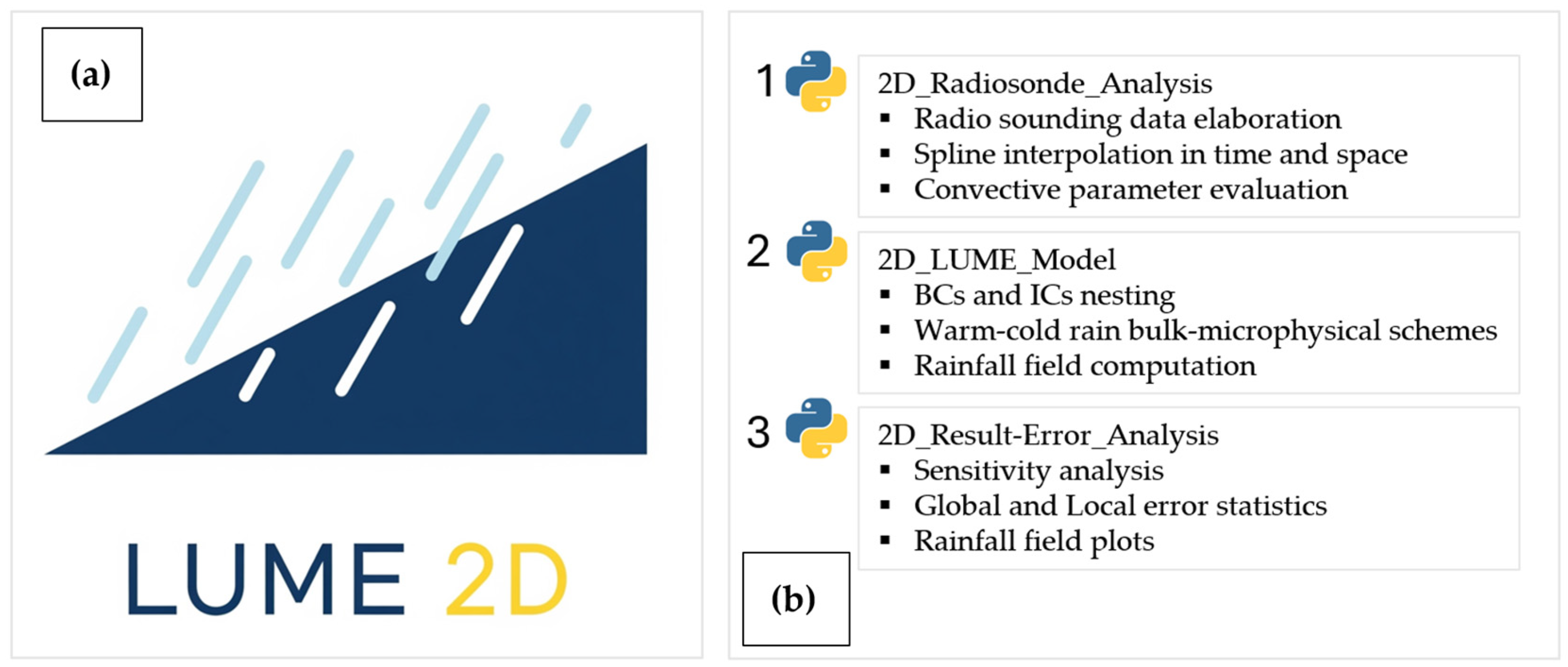
Figure 1. LUME 2D logo (a) and the scheme of Python code (b) where the three main sections are distinguished.
Meteorology 04 00028 g001
Figure 2. Warm (red box) and cold (blue boxes) bulk-microphysical schemes adopted in LUME 2D from the COSMO model: qv (vapour); qc (condensed); qr (rain); qs (snow); and qh or qg (hail–graupel), expressed in mm = l m−2 ≈ kg m−2.
Meteorology 04 00028 g002
Figure 3. (a) Geopotential height (solid lines) at the isobaric level of 500 hPa and temperature (coloured shading) at the isobaric level of 850 hPa at 12 UTC on 16 April 2025. Note the vigorous “Hans” depression located on the sea in front of the Côte d’Azur and the Ligurian Riviera di Ponente; (b) temperature and wind map at 850 hPa at 06 UTC on Thursday, 17 April across Northern Italy, from [31]. (c) Localisation of the Piedmont region with respect to the Alps and Apennines mountain ranges in Italy, and (d) a magnification of the area of Piedmont with the four mountain ranges (Southern, Western, and Maritime Alps and North Apennines) surrounding the case-study area.
Meteorology 04 00028 g003aMeteorology 04 00028 g003b
Figure 4. A comparison of the cumulated rainfall during the 15–17 April 2025 event (a) and during 5–6 November 1994 (b). It can be noted that there are similarities between the 2 events in terms of magnitude (i.e., total cumulates) and rainfall spatial distribution, from [31]. In (c), the position (orange points) of 56 investigated rain gauges across the Piedmont region during the April 2025 event is shown. The green box represents the computational domain considered for LUME 2D simulations.
Meteorology 04 00028 g004
Figure 5. (a) The radiosonde station’s location considered for atmospheric state reconstruction through interpolation techniques (red box, “enlarged domain”). In the yellow box the location of the “computational domain” adopted in this study is shown, from which the digital elevation model is extracted [57], resampled at 2 km resolution (b). In (c), the schematization of the interactions between enlarged and computational domains in terms of ICs and BCs is shown.
Meteorology 04 00028 g005aMeteorology 04 00028 g005b
Figure 6. The Hw (blue), the vertically averaged U (green) and the WVF (red) terms for the investigated event at the Novara Cameri radiosonde location are shown. The peak of WVF is synchronous with respect to U, which exhibits a significant increase during the central phase of the event.
Meteorology 04 00028 g006
Figure 7. Wmid-BL (a) and Wmid-JS (b) evaluated within an enlarged domain. On 16 April 2025 at 00:00 UTC, the Piemonte region experienced intense updrafts, enhanced due to boundary-layer pumping and jet stream acceleration.
Meteorology 04 00028 g007
Figure 8. Convective indexes CAPE (a), CIN (b), TT (c), and KI (d) evaluated within an enlarged domain. From 15 to 17 April 2025, the Piemonte region was also affected by isolated convective episodes correctly predicted by convective indexes: apart from CAPE (rather uniform across the domain), CIN, TT, and KI reported an atmospheric environment prone to trigger convective phenomena.
Meteorology 04 00028 g008
Figure 9. pwind (a) and pconv (b) evaluated on 16 April 2025 00:00 UTC within the enlarged domain. Pink data are located across northwestern Italy and Piedmont, in agreement with the areas affected by convective phenomena.
Meteorology 04 00028 g009
Figure 10. Convective precipitation magnitude evaluated by computing the Gi value under the two scenarios ML (a) and MU (b), expressed in terms of rainfall intensity.
Meteorology 04 00028 g010
Figure 11. PE evaluation using the formulations reported within Appendix A: PENoel, PEMarwitz, PEGLM, PEKI, and PEAvg. The fluctuation of PE can be observed across the entire period, with a slight increase during the most intense phase between 15th and 17th April.
Meteorology 04 00028 g011
Figure 12. τc and τf fluctuation across the event, according to the equation presented in Appendix B. The patterns from 1 to 4 ((be)) are very similar, with τc > τf and variation during the most intense phase of the event. Conversely, the condition τc = τf (a) shows a completely different pattern. Dotted lines define the typical range values of 500 s (lower) and 2000 s (upper) for τc and τf parameters.
Meteorology 04 00028 g012
Figure 13. BL fluctuation across the event, according to the equation presented in Appendix C. BL temporal variation normally resembles the day–night cycle, but during intense rainfall events, it may be disturbed, showing a larger variability with respect to flow-blocking conditions as well.
Meteorology 04 00028 g013
Figure 14. Total precipitation fields simulated by warm-rain (a) and cold-rain (b) schemes. The Alpine area, located in the northern Piedmont region, was correctly simulated with the highest rainfall amounts. The peak values (recorded locally) are quite smooth and slightly underestimated (−20/25%), especially for the cold-rain scheme.
Meteorology 04 00028 g014
Figure 15. Total precipitation fields simulated by warm-rain (a) and cold-rain (b) schemes considering the convection activation. Their spatial distributions are very close to the reference data, even though the rainfall total amount is better represented across the floodplains (higher than in no-convection simulations). The Alpine area, located in the northern Piedmont region, was correctly simulated with the highest rainfall amounts. The peak values (recorded locally) are also quite smooth and slightly underestimated (−20/25%) for both warm-rain and cold-rain schemes.
Meteorology 04 00028 g015
Figure 16. Rainfall transformation into snow (a,b) and hail (c,d) for the cold-rain scheme without and with moist convection activated. The former can significantly increase the amount of latent heat released due to increased condensation rates, causing temperature increases and significant snow amounts. Conversely, hail formation increases when moist convection is activated compared to a no-convective simulation.
Meteorology 04 00028 g016
Figure 17. A series comparison of the total cumulated and rainfall intensities among the four rainfall models tested against the reference data for 5 stations across the Piedmont area: Alagna (a), Biella (b), Coazze (c), Piamparato (d), and Talucco (e). Good time-series agreements are observable, especially for total cumulates. In (f) is represented the location of the five stations across the Piedmont region.
Meteorology 04 00028 g017aMeteorology 04 00028 g017b
Figure 18. Error statistics of the cumulated series for the 56 stations investigated. All the indices give average scores > 0.5 and confirm the good performance of the model. Higher scores have been reached for the warm (a) and cold-rain scheme (b) without convection activation, while lower scores for moist convection runs (c,d) were detected.
Meteorology 04 00028 g018
Figure 19. Error statistics of the rainfall intensity series for the 56 stations investigated. All the indices have performed lower than the total rainfall cumulative, giving average scores that are <0.5 but are generally 0.0, confirming the adequate reproduction of the rainfall intensity in the simulations carried out. Higher scores have been reached for the warm (a) and cold-rain (b) schemes without convection activation, while lower scores were evaluated for moist convection runs (c,d).
Meteorology 04 00028 g019aMeteorology 04 00028 g019b
Figure 20. BIAS distribution across the Piedmont area considering the four simulations of Table 6: (a) for warm-rain scheme, (b) for warm-rain + convection scheme, (c) for cold-rain scheme and (d) for cold-rain + convection scheme. A polarised dipole is present, showing a significant overestimation across the floodplain and an underestimation across the Alps Mountain range in the eastern part of the region.
Meteorology 04 00028 g020
Figure 21. NSE evaluated for the cumulated rainfall time-series for the four simulations of Table 6: (a) for warm-rain scheme, (b) for warm-rain + convection scheme, (c) for cold-rain scheme and (d) for cold-rain + convection scheme. NSE values are higher (>0.6) across the Alps mountain range in the eastern part of the region, while they are lower across floodplains (<0.2).
Meteorology 04 00028 g021
Figure 22. NSE was evaluated for the rainfall intensity time-series for the four simulations of Table 6: (a) for warm-rain scheme, (b) for warm-rain + convection scheme, (c) for cold-rain scheme and (d) for cold-rain + convection scheme. NSE values are higher (>0.4) across the Alps mountain range in the eastern part of the region, while they are lower across floodplains (<0.2).
Meteorology 04 00028 g022
Figure 23. Synthetic simulations were carried out using stationary τc = τf, considering the values 200 s (a), 500 s (b), and 2000 s (c). Increasing τi values, total rainfall becomes more diffused across the domain, significantly reducing the peak amount of total rainfall (from >800 mm for 200 s up to ≈300 mm for 2000 s). Time scales have a strong influence on maximum precipitation Pmax (d), confirmed by the SMAPE index, which reduces from 0.5 to 0.4: reducing the timescale, Pmax tends to sharply increase.
Meteorology 04 00028 g023
Figure 24. The relative biases of “cold no-convection” simulation at each rain-gauge location. Across the northeastern mountain sector of the Piedmont region, biases are negative, but with an underestimation of 20–30% with respect to the reference gauges. Conversely, across flood plains, the overestimation may reach up to 60–80%, lowering model skills.
Meteorology 04 00028 g024
Table 1. The radiosonde stations’ names considered for atmospheric state reconstruction through interpolation techniques in the Northern Italy area.
Radiosonde NameLocationNationWMO Code
Novara CameriNovaraItaly16064
Cuneo LevaldigiCuneoItaly16117
San Pietro CapofiumeBolognaItaly16144
Pratica di MareRomaItaly16245
UdineUdineItaly16045
PayernePayerneSwitzerland06610
AjaccioAjaccioFrance07761
InnsbruckInnsbruckAustria11120
MuenchenMuenchenGermany10410
Table 2. Atmospheric variables and parameters utilised in LUME 2D.
Variable or ParameterSymbolUnit of Measure
Reference Temperature (z = 0 m) T r e f [°C]
Environmental Lapse Rate γ e n v [°C m−1]
Moist Lapse Rate Γ m o i s t [°C m−1]
Brunt Vaisala Frequency N m o i s t [s−1]
Reference Air Density ρ r e f [kg m−3]
Reference Humidity R H r e f [-]
Wind Velocity U [m s−1]
Wind Direction D [°]
Convective Available Potential Energy C A P E [J kg−1]
Convective Inhibition C I N [J kg−1]
Low Convective Layer L C L [m]
Level of Free Convection L F C [m]
Equilibrium Layer E L [m]
Precipitable Water P W [mm]
Precipitation Efficiency P E [-]
Convective Generator term G 1 and G 2 [mm h−1]
Boundary Layer Height B L [m]
Wind Vapour Flux W V F [kg s−1 m−1]
Water-Scale Height H w [m]
Conversion and Fallout time-scale terms τ c   and τ f [s]
Table 3. The triggering functions based on CI evaluated in the study. In the table, the minimum and maximum value of CI scales and the thresholds adopted for moist convection activation are reported.
CINameMin ValueMax ValueThreshold
CAPE-CAPEv
[J kg−1]
Convective Available Potential Energy
(using T and virtual T)
04000>1000
CIN-CINv
[J kg−1]
Convective Inhibition
(using T and virtual T)
−1000>−50
LI-Liv
[-]
Lifted Index
(using T and virtual T)
−73<−3
TT [-]Total Totals4060>50
KI [-]K-Index1050>26
SI [-]Showalter Index−74<−2
DCI [-]Deep Convective Index1050>30
Table 4. Local extreme rainfall recorded across the Piedmont region during 15–17 April 2025. The locations of the stations are reported in the subsequent Figure 4c.
Rain-Gauge Stations—ARPA PiemonteTotal Rainfall [mm]ID
Gressoney-St-Jean–Lago Seebna (Valle del Lys, Aosta)643.31
Trivero-Camparient (Val Sessera, Biella) 570.62
Lillianes-Granges (Valle del Lys, Aosta) 567.23
Boccioleto (Val Sesia, Vercelli) 565.04
Santuario di Oropa (Biella) 509.55
Carcoforo (Val Sesia, Vercelli) 473.46
Corio-Pian Audi (Val Malone, Torino)465.97
Valstrona-Sambughetto (VCO)462.28
Andrate-Alpe Pinalba (between Ivrea e Biella) 460.49
Montecrestese-Lago Larecchio (Valle Isorno, VCO)458.410
Table 5. Global error statistics evaluated for LUME 2D during the sensitivity analysis, applying the warm-rain scheme. Simulations from 1 to 10 different formulae of τi and BL were tested, while 10 to 12 report reference simulations fixing τc = τf.
N_SimCodeTypeMEANsMEANrSQMsSQMrBIAS_addBIAS_mulRMSE_addRMSE_mulAISSMAPECC
[-][-][-][mm][mm][mm][mm][mm][mm][mm][mm][mm][-][-]
1RaML_Sv0_Mt0_Co0_Sr0_Ta0_Bl0A190.21263.3866.07125.7773.1811.05138.4323.38246.040.450.907
2RaML_Sv0_Mt0_Co0_Sr0_Ta0_Bl1A226.23263.3894.89125.7737.154.99131.4824.06197.680.440.894
3RaML_Sv0_Mt0_Co0_Sr0_Ta1_Bl1A244.25263.3833.53125.7719.13−1.86121.0323.22165.240.40.912
4RaML_Sv0_Mt0_Co0_Sr0_Ta1_Bl3A259.42263.3838.33125.773.96−4.7611423.31146.030.380.921
5RaML_Sv0_Mt0_Co0_Sr0_Ta1_Bl5A228.47263.3825.6125.7734.910.9129.0523.52188.380.430.905
6RaML_Sv0_Mt0_Co0_Sr0_Ta4_Bl3A259.6263.3838.31125.773.78−4.76117.3723.79149.70.390.916
7RaML_Sv0_Mt0_Co0_Sr1_Ta4_Bl3M410.71263.38133.32125.77−147.33−30.49204.6741.63424.120.50.912
8RaML_Sv0_Mt0_Co0_Sr1_Ta4_Bl1M362.72263.38123.74125.77−99.33−21.55181.1136.47338.460.460.891
9RaML_Sv0_Mt0_Co0_Sr0_Ta0_Bl3M361.89263.38105.08125.77−98.51−22.05152.5733.08306.210.430.927
10RaML_Sv0_Mt0_Co0_Sr0_Ta0_Bl5M280.82263.3876.19125.77−17.43−7.88136.1627.57189.040.430.891
11RaML_Sv0_Mt0_Co0_Sr0_Ta0_Bl11M411.28263.38125.88125.77−147.9−30.49190.3439.87408.60.50.932
12RaML_Sv0_Mt0_Co0_Sr0_Ta0_Bl12M370.35263.38103.15125.77−106.97−23.95155.5133.98320.410.440.93
13RaML_Sv0_Mt0_Co0_Sr0_Ta0_Bl13A255.12263.3828.98125.778.26−4.25119.9324.09156.530.40.912
Table 6. Global error statistics evaluated for LUME 2D applying the four rain microphysical schemes: warm rain and cold rain, without and with moist convection activated.
N_SimCodeSimTypeMEANsMEANrBIAS_addBIAS_mulRMSE_addRMSE_mulAISSMAPECC_2
[-][-][-][-][mm][mm][mm][mm][mm][mm][mm][-][-]
1RaML_Sv0_Mt0_Co0_Sr0_Ta1_Bl3warm_no_cA259.42263.383.96−4.7611423.31146.030.380.921
2RaML_Sv0_Mt1_Co0_Sr0_Ta1_Bl3cold_no_cA258.26263.385.12−4.75113.222.79145.860.380.922
3RaML_Sv0_Mt0_Co1_Sr0_Ta1_Bl5warm_cM270.33263.38−6.95−7.25127.2726.59168.060.420.9
4RaML_Sv0_Mt1_Co1_Sr0_Ta1_Bl5cold_cM269.94263.38−6.56−7.25127.1826.58167.570.420.901
Table 7. BIAS was evaluated for the station reported in Table 4, considering the best simulation of LUME 2D (n°2 of Table 6). As can be observed, a negative BIAS (i.e., model underestimation) in the order of 100–150 mm (20–30% of the total rainfall amount) was evaluated across the Alps in the northeastern sector of Piedmont. Boccioleto (*) and Oropa (**) are the stations poorly reconstructed by LUME 2D, with underestimation reaching up to 40%.
Rain-Gauge Stations—ARPA PiemonteTotal Rainfall [mm]Total Rainfall LUME 2D [mm]BIAS [mm]Relative BIAS [-]
Gressoney-St-Jean–Lago Seebna (Valle del Lys, Aosta)643.3410−233.3−0.36
Trivero-Camparient (Val Sessera, Biella) 570.6400−170.6−0.29
Lillianes-Granges (Valle del Lys, Aosta) 567.2396−171.2−0.30
Boccioleto (Val Sesia, Vercelli) 565310 (*)−255−0.45
Santuario di Oropa (Biella) 509.5290 (**)−219.5−0.43
Carcoforo (Val Sesia, Vercelli) 473.4345−128.4−0.27
Corio-Pian Audi (Val Malone, Torino): 465.9320−145.9−0.31
Valstrona-Sambughetto (VCO): 462.2275−187.2−0.39
Andrate-Alpe Pinalba (between Ivrea e Biella) 460.4340−120.4−0.26
Montecrestese-Lago Larecchio (Valle Isorno, VCO)458.4323−135.4−0.29
Table 8. The main practical indications for the model implementation discussed in this paragraph and the strategies implemented in LUME 2D.
TopicLUME 2D Implementation Strategies
IC and BC setupSpecified from the enlarged domain, BC functions of WVF; updated hourly.
Reanalysis and forecast modes setupReanalysis (using recorded RAOBS) and forecast (using forecasted RAOBS from global forecasting models).
Effect of DEM resolution on computationsInfluence upslope–downslope flux; suggested resolution ≈ 1–2 km.
Spatial Extension of Computational DomainAny, but the suggested regional scale is recommended (≈100,000 km2).
Disclaimer/Publisher’s Note: The statements, opinions and data contained in all publications are solely those of the individual author(s) and contributor(s) and not of MDPI and/or the editor(s). MDPI and/or the editor(s) disclaim responsibility for any injury to people or property resulting from any ideas, methods, instructions or products referred to in the content.