Abstract
In astronomy, understanding the evolutionary trajectories of galaxies necessitates a robust analysis of their star formation histories (SFHs), a task complicated by our inability to observe these vast celestial entities throughout their billion-year lifespans. This study pioneers the application of the Kullback–Leibler Importance Estimation Procedure (KLIEP), an unsupervised domain adaptation technique, to address this challenge. By adeptly applying KLIEP, we harness the power of machine learning to innovatively predict SFHs, utilizing simulated galaxy models to forge a novel linkage between simulation and observation. This methodology signifies a substantial advancement beyond the traditional Bayesian approaches to Spectral Energy Distribution (SED) analysis, which are often undermined by the absence of empirical SFH benchmarks. Our empirical investigations reveal that KLIEP markedly enhances the precision and reliability of SFH inference, offering a significant leap forward compared to existing methodologies. The results underscore the potential of KLIEP in refining our comprehension of galactic evolution, paving the way for its application in analyzing actual astronomical observations. Accompanying this paper, we provide access to the supporting code and dataset on GitHub, encouraging further exploration and validation of the efficacy of the KLIEP in the field.
1. Introduction
In recent times, many transfer problems have arisen, and various methods exist to solve them. We can broadly classify these into three categories. First is supervised domain adaptation, where only a few labeled target data are available [,,,,,]. Second is semi-supervised domain adaptation, where, in addition to these labeled data, a large amount of unlabeled data are available [,,,,]. Finally, we have unsupervised domain adaptation, where only unlabeled data are available in the target [,,,,]. Researchers have shown that adding target labels can increase the performance of the model []. This setting is also the most encountered in practice [], as it is often possible to label at least a few target samples.
However, there are cases in which obtaining supervised data is not possible. Such is the case of the present astrophysics problem of SFH prediction. Here, we aim to learn the history of our universe through the evolution of its galaxies’ masses throughout their individual histories. We try to obtain this history from the radiation that reaches us on Earth—the Spectral Energy Distribution (SED), a function of the brightness of a galaxy with the wavelength of observation.
As galaxies evolve over billions of years, capturing the complete Spectral Energy Distribution (SED) of any single galaxy over time remains a formidable challenge. Astrophysicists have developed models based on physically motivated mechanisms to construct artificial star formation histories (SFHs) and their corresponding radiation outputs. These models, aiming to establish a reliable correspondence between observed radiation and underlying SFHs, predominantly employ classic Bayesian approaches such as ProSpect [], MagPhys [,], CIGALE [,], BAGPIPES [,], and Prospector [,].
While these Bayesian models are instrumental in inferring SFHs from observed SEDs, they are not without limitations. Their performance can be constrained by the simplifications and assumptions inherent in their design, such as the parametrization of dust models, stellar population synthesis, and the treatment of nebular emission. These simplifications, while necessary for computational feasibility, can lead to discrepancies between predicted and actual SFHs, especially when the models are applied to data beyond their calibration range. Moreover, the evaluation of these models often relies on comparisons with synthetic data or specific observational datasets, which may not fully represent the diversity and complexity of galaxy populations in the universe.
Deep neural networks (DNNs) have emerged as powerful tools in various astronomical domains, demonstrating significant success in addressing complex and large-scale data analysis challenges. In the field of exoplanet discovery, DNNs have been employed to identify exoplanetary signals from vast amounts of stellar light curve data [,,]. Similarly, in the realm of cosmology, DNNs have facilitated the analysis of cosmic microwave background data to extract insights about the early universe [,,]. Moreover, in the study of gravitational waves, these networks have accelerated the detection and characterization of gravitational wave signals, contributing to our understanding of astrophysical events [,,]. The application of DNNs extends to the classification and analysis of galaxies, where they help in morphological classifications [,] and redshift estimations [,]. Specialized neural networks have been used for improving observing schedules at astronomical observatories [,], inferring redshifts from a collection of observed temporal and spectral features of gamma ray bursts [,], and extracting probabilistic stellar properties from their observed spectra [,], showcasing their versatility and expanding their utility in various branches of astronomy.
The challenge of “domain shift”—the discrepancy between the training domain of models and the target observational domain—further complicates the application of these models to real-world data. This is evident even with DNN-based approaches, like mirkwood [] and beyond-mirkwood [], which, while promising, also struggle with domain shift when applied to real galaxies. To address these challenges, this work explores unsupervised domain adaptation, aiming to refine the extraction of SFHs from individual galaxies without the constraints of physical model simplifications and conventional SED-fitting techniques’ parametrizations.
We leverage cosmological, hydrodynamic simulations such as eagle [], illustristng [,] and simba [], which simulate the universe’s evolution from shortly after the Big Bang to the present day. These simulations offer a framework to study galaxies as proxies for real ones, enabling direct comparisons with observational data and helping to refine our models’ predictive capabilities. Through unsupervised domain adaptation, we seek to enhance the generalization of SFH prediction models, ensuring they remain robust across varying galactic environments, thereby enriching our understanding of the universe’s evolution.
2. Data
Our training and test datasets consist of SEDs from three state-of-the-art cosmological galaxy formation simulations, where the true physical properties are known—including their true star formation histories. Simba [], Eagle [,,], and IllustrisTNG [], with 1688, 4697, and 9633 samples, respectively, together constitute a diverse sample of galaxies with realistic growth histories. Specifically, we select galaxies at a redshift of 0—this corresponds to simulated galaxies at the “present” epoch. Each SED is comprised of 20 measurements of the “brightness” of a galaxy at different wavelength, in the form of flux density (with units of Jansky) and are the co-variates or features that we train/learn on. The outputs/labels are star SFH time series vectors with 29 scalar elements, in units of solar mass per year (M⊙ yr−1).
The SFH for a galaxy informs us about the net stellar mass generated as a function of time—sum of masses of all stars born, less the sum of stellar mass lost in stellar winds as stars age and eventually die. In other words, SFHs are plots of the star formation rates (SFRs) of galaxies against the lookback time, which for galaxies at extends from 0 to the very age of our universe (∼13.8 Gyrs). By stacking (adding) together SFHs of several thousand galaxies from a simulation, and dividing by the volume of the simulated box (i.e., the size of the simulated universe), we can derive the cosmic star formation rate density (CSFRD), which is a well-studied global property of our universe. Astrophysicists aim to tune various physical properties in any given simulation until the CSFRD plot derived from it matches closely to the most widely accepted one derived from observations [].1
In this study, our analysis is confined to galaxies at a redshift of , which represents the current state of the universe. This temporal constraint poses a significant limitation when it comes to deriving the Cosmic Star Formation Rate Density (CSFRD), which requires a comprehensive temporal perspective, encompassing a wide range of redshifts to accurately reflect the universe’s star formation history over billions of years. The CSFRD integrates the star formation rates across all galaxies over time and space, offering a global view of star formation activity throughout the history of the universe. However, with our dataset restricted to , we lack the longitudinal depth needed to construct this global metric, as we only observe the galaxies’ most recent star formation activities.
To navigate this limitation, we pivot our analysis to leverage SFHs, which are the summations of individual star formation histories from a collection of galaxies at a single time point. While SFHs do not provide the extensive temporal insight that CSFRD offers, they still enable us to aggregate star formation activities across a wide array of galaxies at the present epoch. This approach allows us to capture a snapshot of the cumulative star formation activity within the observable universe at , providing valuable insights into the current state of galaxy evolution and the prevailing star formation processes. By focusing on SFHs, we adapt our methodology to the available data, ensuring that our analysis remains robust and informative despite the inherent constraints of our dataset.
We sequentially train on any two of these simulated datasets, and predict on the third, thus giving us three sets of source- and target domain data and results.
3. Methodology
We consider the problem of the prediction of SFH, where the learner has access to a dataset encoding the radiations of n galaxies with p as the number of filters/wavelength-bins, and a dataset giving the corresponding SFH for each galaxy with T as the time length of the history (see Figure 1). Each SED (row of X) is comprised of measurements of the “brightness” of a galaxy at different wavelengths, in the form of flux density (with units of Jansky) (see Figure 2). , and the sampling is slightly different for each of the three simulations2.
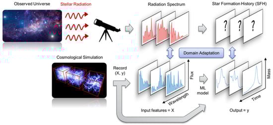
Figure 1.
Radiation spectra with corresponding star formation histories can be recorded from cosmological simulation to form a dataset . Here, X is the collection of spectra in tabular form, each column containing the flux values in a photometric band. y is the collection of star formation histories in tabular form, each column containing stellar mass formed in a historical time band. Our machine learning model is trained on known X and y from computer simulations. Owing to the domain shift between real radiation spectra and simulated ones, domain adaptation is used to adapt the learned machine learning model to real observations.
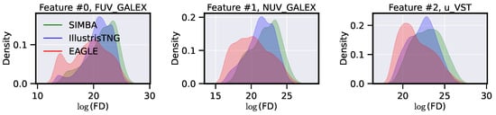
Figure 2.
Kernel density estimate plots of the log of flux densities (FD) for the first three features. The feature names at the top of each plot are the names of the filters, each centered at a different wavelength, in which photometry was simulated. We notice that for the three features shown here, all three simulations share the same support, which justifies our decision of using KLIEP.
Below are our pre-processing steps:
- First, we create three sets of experiments to ensure a comprehensive evaluation across all simulations. In each set, we utilize galaxies from two of the three simulations—simba, illustristng, and eagle—as our training and validation sets, and galaxies from the remaining simulation as our test set. This approach is designed to emulate real-world scenarios where the ground truth is unknown, and we must rely on models trained on different but related data. The 9:1 split between training and validation sets was chosen as a conventional starting point in machine learning practice, providing a substantial amount of data for training while reserving a reasonable subset for validation. The choice of this split ratio is somewhat arbitrary and commonly used in the field, offering a balance between learning from a large training set and having enough data to validate the model’s performance effectively. While other split ratios or more complex cross-validation schemes might influence the model’s performance, the impact of such variations is beyond the scope of this initial study and is earmarked for future exploration. This study aims to establish a baseline understanding of how well models trained on one set of simulated galaxies generalize to another, using a straightforward and widely accepted split ratio for initial experiments.
- Second, we normalize each SFH time series (each row of Y) by its sum and store the resultant normalized SFH (SFHnorm) and the sum (SFHsum) separately. This normalization is crucial given the vast dynamic range of star formation histories observed across different galaxies. See Appendix D): SFH curves have a large variety of scales, some increasing to more than 100, whereas others never increase over . Without normalization, galaxies with intrinsically high star formation rates could dominate the learning process, overshadowing subtler trends in galaxies with lower rates. By scaling each SFH time series, we facilitate the model’s ability to learn the underlying patterns in the SFHs, independent of their absolute scale. The learning of the SFHs is now decoupled in the learning of SFHnorm and SFHsum.However, this approach also introduces considerations that must be acknowledged. First, the normalization step assumes that the shape of the SFH curve is more informative than its absolute scale, which may not always hold true, especially if the scale itself carries significant astrophysical information. Second, this method may amplify the noise in SFHs with very low sums, potentially impacting the model’s ability to learn meaningful patterns from these histories. Additionally, decoupling the learning of SFHnorm and SFHsum assumes that these two components are independent, which may not fully capture the complexities of galaxy evolution, where the total star formation and its distribution over time could be interrelated. While this normalization facilitates the learning process by standardizing the range of input features, it is essential to consider these aspects when interpreting the model’s outputs and in future investigations to refine the approach.
- Third, we further ease the learning of the SFHnorm by reducing the curves to their first 3 Kernel-PCA (Principal Component Analysis) components [,]. This choice is predicated on a series of comparative analyses where Kernel-PCA demonstrated superior performance in preserving the essential characteristics of the SFH time series when compared to linear PCA [,] and discrete wavelet transform (DWT) [,]. Our evaluation focuses on the capacity of each method to reconstruct the original time series while maintaining its significant features. The effectiveness of this reconstruction is quantitatively assessed using the DILATE loss metric (Distortion Loss including shApe and TimE) [], which incorporates both dynamic time warping (DTW) and the temporal distortion index (TDI) to evaluate the similarity between the original and reconstructed time series.During our experimentation, Kernel-PCA consistently outperforms its counterparts by achieving lower DILATE loss scores, suggesting that it retains more of the original series’ structural and temporal integrity. Specifically, in our tests, Kernel-PCA exhibits a more robust ability to capture non-linear patterns within the SFH data, a key aspect given the complex nature of these time series. The selection of the number of components (3) is based on a variance-explained criterion, where we aim to retain at least of the variance within the validation set, ensuring a balance between dimensionality reduction and information retention. This process and its outcomes are further detailed in Appendix A and visually represented in Figure A1, where we compare the reconstruction fidelity of SFH time series using different methods, clearly illustrating the advantage of Kernel-PCA advantage in our specific application context.
- Fourth, we normalize the input features (the columns from X) via log-scaling, and follow this up by standard scaling normalization. In Figure 2, we visualize the log-scaled flux densities, in units of Janskies, for all three simulations, in 3 out of 20 filters.
- Finally, we derive KLIEP weights for the training samples in all three experiments. The Kernelized Learning for Independence (KLIEP) algorithm [] is employed to adjust the weights of the training samples to minimize the Kullback–Leibler (KL) divergence between the source and target distributions. This instance-based domain adaptation approach is chosen due to its robustness in handling regression domain adaptation challenges and its effectiveness in mitigating negative transfer [,,,].
In our implementation, we carefully select the kernel and bandwidth parameters for KLIEP. The kernel type (Gaussian) and the bandwidth are crucial hyperparameters in this context. We conduct a grid search over a range of bandwidth values to identify the optimal setting that minimizes the KL divergence between the adapted source domain and the target domain. This process is detailed in Appendix B, where we showcase the parameter selection procedure for one of the experiments, demonstrating how the bandwidth impacts the effectiveness of domain adaptation.
Additionally, for the kernelPCA component, we explore a range of hyperparameters, specifically the kernel type and the parameter in the Gaussian kernel, to find the best combination that allows for the most accurate reconstruction of the SFH time series. While Figure A1 illustrates examples with values of 1 and 3, a broader range of values were examined to ensure robustness in the selection process. The effectiveness of each parameter setting is evaluated using the DILATE loss metric, providing a quantitative measure of the reconstruction’s fidelity compared to the original SFH.
We also visually observe from the marginal distributions for the 20 input filters that all domains have the same support in the feature space. In other words, we ensure that the distributions of input features across the different domains (simulations) cover similar ranges. This is crucial for the application of KLIEP, as the method assumes that the support of the source and target distributions overlap. To visually assess this, we examine the marginal distributions of the 20 input filters across the three simulations. If the distributions of each feature across the simulations show considerable overlap, we consider the support to be “the same” for practical purposes. This overlap ensures that the reweighing process by KLIEP is meaningful and grounded in comparable data ranges across domains. A detailed illustration of this overlap is provided in Appendix B and Figure A2, where kernel density estimates or histograms of feature distributions from different simulations are juxtaposed to highlight their common support.
For each of SFHkPCA and SFHsum, we employ an ensemble of 50 4-layer feed-forward deep neural networks with dropout and 256 nodes in each layer, using ReLU as the activation function and Adam [] as the optimizer with a learning rate of . The networks are trained for 200 epochs with early stopping to prevent overfitting. Employing multiple DNNs allows us to derive probability distributions over the SFH predictions, offering a nuanced understanding of the model’s performance and the uncertainty in its predictions. The choice of a 4-layer feed-forward DNN with 256 nodes per layer is guided by a balance between model complexity and computational efficiency, as well as empirical validation. The architecture is deep enough to capture the complex relationships between input features and the target SFHs, yet not so large as to risk overfitting given the available data size. The number of nodes is selected to provide sufficient capacity for learning intricate patterns without unnecessarily increasing the parameter count, which could lead to longer training times and require more data to avoid overfitting. This configuration is empirically tested against other architectures with varying depths and widths. The chosen setup consistently offers a good trade-off between learning capability and generalization performance, evidenced by the validation loss metrics and the model’s ability to predict SFHs on unseen data from the test simulation.
4. Results
The evaluation of the SFH outputs generated by our machine learning model is conducted through two primary methods:
- The SFH predictions for individual galaxies within the test set are compared against their corresponding true SFHs. This direct comparison provides a granular assessment of the model’s predictive accuracy on a per-galaxy basis.
- The aggregate predicted star formation histories SFH, representing the sum of SFHs across all galaxies within a simulation, are compared to the true SFHs. The true SFH serves as an essential benchmark, reflecting the cumulative star formation activity and validating the simulation’s input physics. Observational evidence indicates that the universe’s star formation peaked approximately 2 billion years after its inception [], a critical detail that all hydrodynamical simulations must replicate to be considered accurate. Ensuring concordance between the SFH derived from our model and that from established simulations underpins the robustness of our approach. This alignment not only corroborates our model’s efficacy but also facilitates the fine-tuning of its architecture, loss functions, and hyperparameters in response to any discrepancies. Additionally, this comparison sheds light on potential systematic biases when the model is trained on one simulation and tested on another.
In Figure 3, we plot the true and derived SFH curves for the three distinct test datasets (Simba, IllustrisTNG, and Eagle), where the training data consist of samples from the other two simulations. In these cases, the resulting sample SFHs (and thus SFH) are most deviant from their ground truth vectors. This is unsurprising, as the different simulations have intrinsically different sample SFHs; this is a known difference between different simulations (as shown in Figure A1 of []).
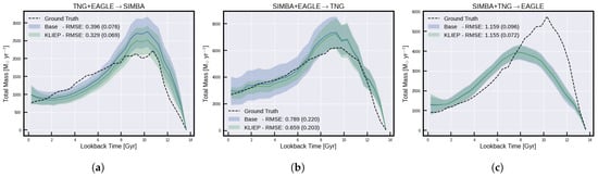
Figure 3.
Global SFH predictions for the three experiments. The curves correspond to the sums over all SFHs or predicted SFHs. (a) is when we train on illustristng and eagle, and test on simba; (b) is when we train on eagle and simba, and test on illustristng; (c) is when we train on simba and illustristng, and test on eagle.
Table 1 and Table 2 show the five metrics tested within this work —mean absolute error (MAE), root mean squared error (RMSE), bias error (BE), dynamic time warping (DTW), and temporal distortion index (TDI)—for average predictions of SHF, and for SFH, respectively. These metrics are chosen for their ability to capture different aspects of the model’s accuracy and reliability in predicting SFHs. For instance, MAE and RMSE provide insights into the average prediction errors, while DTW and TDI offer a nuanced view of the model’s ability to capture the temporal dynamics of SFHs. Figure A4, Figure A5 and Figure A6 show examples of true and derived SFHs for individual galaxies within the simulations using KLIEP. Based on the five metrics, each row shows an example of the best-performing galaxy output on the left and the worst-performing galaxy on the right. It is noteworthy that the best and worst performers vary across different metrics, underscoring the distinct ways in which each metric evaluates time-series data. Consequently, while it is challenging to designate a single metric as the definitive loss function for minimization, RMSE is selected as the primary metric for several figures within this paper, facilitating a high-level understanding of the model’s performance.

Table 1.
Forecasting results for individual SFHs. The first column gives the target domain IllustrisTNG, Eagle or Simba, and the two other domains are used as source domains. The computed metrics between each individual SFH prediction and the corresponding ground truth are averaged in the target domain. The , , and quantile values are drawn from the 50 predictions per galaxy, corresponding to the 50 neural networks used. The leading method between UDA and no-UDA (baseline) is shown in bold. Downward arrows for metrics imply that lower values are better.
Table 2.
Forecasting results for SFH (total star formation history). The first column gives the target domain IllustrisTNG, Eagle or Simba, and the two other domains are used as source domains. Predictions for all samples in the target domain are summed and compared to the true SFH according to the different metrics. The , , and quantile values are drawn from the 50 predictions per galaxy, corresponding to the 50 neural networks used. The leading method between UDA and no-UDA (baseline) is shown in bold. Metrics are scaled (MAE × 1000, RMSE × 1000, BE × 1000, DTW × 1000 for readability. Downward arrows for metrics imply that lower values are better.
Another observation made from these three figures is how well our technique can reproduce the stochastic nature of the simulated galaxies’ SFHs. As star formation can be an incredibly stochastic process (as is clear from examples such as the top-left panel in Figure A4 and the top-left panel in Figure A5), SFHs can regularly fluctuate between high and low values. In general, we find that such stochastic SFHs are poorly recovered. For the sake of galaxy property analysis, the accurate recovery of overall SFH trends is more important than the recovery of individual star formation rate (SFR) epochs. In the bottom-right panel of Figure A4, for example (galaxy index 333), it can be seen that there is a star formation event early on at ∼10–12 Gyr, and then a secondary star formation event from ∼2 Gyr to the present day. Recovering these two main epochs is more crucial than correctly recovering the individual SFR peaks within each epoch. One way of achieving this is to temporally smooth the SFHs of individual galaxies prior to training and testing. We can justify such smoothing of simulated features given that we would never expect the derived SFHs for observed galaxies (the ultimate aim of this work) to reproduce such short-scale stochastic features. As an example of this, see Figure A4 of Robotham et al. [], where “good” fits to the SFHs from the semi-analytic model Shark [] from the SED-fitting code ProSpect do not recover the stochastic SFHs.
To further contextualize our findings, we compare KLIEP with other popular domain adaptation methods3 in Appendix C—Margin Disparity Discrepancy (MDD) [], Discriminative Adversarial Neural Network (DANN) [], Kernel Mean Matching (KMM) [], Correlation Alignment (CORAL) [], and Deep Correlation Alignment (DeepCORAL) []. KMM, like KLIEP, is also an instance-based method, while the rest are feature-based methods. This comparison aims to highlight the strengths and potential areas for enhancement of our domain adaptation technique relative to other strategies. The curious reader will notice that while at times CORAL methods outperform KLIEP, this is very much a data-dependent result, and KLIEP provides the most reliably acceptable results across datasets, making it more generalizable. This is most clearly apparent in Figure A3.
5. Future Work
The results presented here are only one part of a continuing effort to apply sophisticated data-driven methods to SED fitting, a crucial first step for extracting galaxy properties. In future work, we will explore advanced multi-source domain adaptation approaches [,], which should more robustly account for the presence of multiple source-domain datasets as well as adaptively reweigh the training samples depending on the prediction task, thus providing higher quality results.
We are also actively analyzing and attempting to correct systematic biases induced by our various design choices. How do our SFH inferences for galaxies of low mass compare to those of high mass? Is our modeling sufficient to accurately infer SFH from both old and young galaxies, unlike traditional parametric approaches, which suffer at earlier epochs in the universe’s history? Answers to such questions will enable us to discover and correct potential biases in our predictions.
Finally, we also plan on vastly increasing the size of our simulated data to account for the immense diversity in the physics of galaxy formation and evolution modeling–different initial mass functions (IMFs) (for example [,,]), nebular emission models (for example []), and mass–metallicity relationships (such as those presented by [,,]), among others. While this task has a relatively longer horizon—generating and saving new simulations is a compute-intensive task—it is crucial to undertake before data-driven methods such as the one proposed in this paper become trusted by astronomers.
Author Contributions
Conceptualization, S.G. and A.d.M.; methodology, S.G. and A.d.M.; software, S.G., A.d.M. and G.R.; validation, S.G., A.d.M., S.B. and G.R.; formal analysis, S.G., A.d.M. and S.B.; investigation, S.G., A.d.M. and S.B.; resources, S.G., A.d.M. and G.R.; data curation, S.G. and A.d.M.; writing—original draft preparation, S.G. and A.d.M.; writing—review and editing, S.G., A.d.M., S.B. and G.R.; visualization, S.G., A.d.M. and S.B.; supervision, S.G., A.d.M. and S.B.; project administration, S.G. and A.d.M.; funding acquisition, None. All authors have read and agreed to the published version of the manuscript.
Funding
This research received no external funding.
Conflicts of Interest
The authors declare no conflicts of interest.
Appendix A. Selection of Time Series Reduction Method
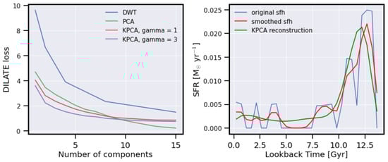
Figure A1.
Comparison of SFH reduction approaches for simba. On the left, the evolution of DILATE loss between the true SFH and the reconstructed signal after one of the three transformations: DWT, PCA, kernelPCA. On the right, reconstructed signal for one of the simba SFH. The sawtooth features in the raw SFH are a product of finite sampling and limited data; hence, we present a second plot (red) which is a smoothed version and a better presentation of reality.
Appendix B. KLIEP Reweighing
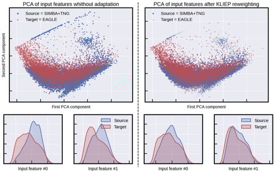
Figure A2.
KLIEP brings different domains closer by reweighing source samples. Top: Scatter plot of the first two PCA components in the input space. Bottom: KDE plots of log of the first two features. These are randomly selected to illustrate the impact of KLIEP, and do not correspond 1:1 to the 2 PCA components.
Appendix C. Extended Results
Table A1.
Forecasting results for individual SFHs, with IllustrisTNG and Simba as source domains and Eagle as the target domain. Predictions for all samples in Eagle have been averaged, and , , and quantile values are drawn from the 50 predictions per galaxy, corresponding to the 50 neural networks used. Downward arrows for metrics imply that lower values are better.
| RMSE (↓) | MAE (↓) | BE (↓) | DTW (↓) | TDI (↓) | |
|---|---|---|---|---|---|
| Base | |||||
| KLIEP | |||||
| MDD | |||||
| DANN | |||||
| DeepCORAL | |||||
| KMM | |||||
| CORAL |
Table A2.
Forecasting results for SFH (total star formation history) with IllustrisTNG and Simba as source domains and Eagle as the target domain. Predictions for all samples in Eagle are added, and , , and quantile values are drawn from the 50 predictions per galaxy, corresponding to the 50 neural networks used. Metrics are scaled (MAE × 1000, RMSE × 1000, BE × 1000, DTW × 1000 for readability. Downward arrows for metrics imply lower values are better.
| RMSE (↓) | MAE (↓) | BE (↓) | DTW (↓) | TDI (↓) | |
|---|---|---|---|---|---|
| Base | |||||
| KLIEP | |||||
| MDD | |||||
| DANN | |||||
| DeepCORAL | |||||
| KMM | |||||
| CORAL |
Table A3.
Forecasting results for individual SFHs, with IllustrisTNG and Eagle as source domains and Simba as the target domain. Predictions for all samples in Simba have been averaged, and , , and quantile values are drawn from the 50 predictions per galaxy, corresponding to the 50 neural networks used. Downward arrows for metrics imply that lower values are better.
| RMSE (↓) | MAE (↓) | BE (↓) | DTW (↓) | TDI (↓) | |
|---|---|---|---|---|---|
| Base | |||||
| KLIEP | |||||
| MDD | |||||
| DANN | |||||
| DeepCORAL | |||||
| KMM | |||||
| CORAL |
Table A4.
Forecasting results for SFH (total star formation history) with IllustrisTNG and Eagle as source domains and Simba as the target domain. Predictions for all samples in Simba have been added, and , , and quantile values are drawn from the 50 predictions per galaxy, corresponding to the 50 neural networks used. Metrics are scaled (MAE × 1000, RMSE × 1000, BE × 1000, DTW × 1000 for readability. Downward arrows for metrics imply that lower values are better.
| RMSE (↓) | MAE (↓) | BE (↓) | DTW (↓) | TDI (↓) | |
|---|---|---|---|---|---|
| Base | |||||
| KLIEP | |||||
| MDD | |||||
| DANN | |||||
| DeepCORAL | |||||
| KMM | |||||
| CORAL |
Table A5.
Forecasting results, with Simba and Eagle as source domains and IllustrisTNG as the target domain. Predictions for all samples in IllustrisTNG have been averaged, and , , and quantile values are drawn from the 50 predictions per galaxy, corresponding to the 50 neural networks used. Downward arrows for metrics imply that lower values are better.
| RMSE (↓) | MAE (↓) | BE (↓) | DTW (↓) | TDI (↓) | |
|---|---|---|---|---|---|
| Base | |||||
| KLIEP | |||||
| MDD | |||||
| DANN | |||||
| DeepCORAL | |||||
| KMM | |||||
| CORAL |
Table A6.
Forecasting results for SFH (total star formation history) with Simba and Eagle as source domains and IllustrisTNG as the target domain. Predictions for all samples in IllustrisTNG are added, and , , and quantile values are drawn from the 50 predictions per galaxy, corresponding to the 50 neural networks used. Metrics are scaled (MAE × 1000, RMSE × 1000, BE × 1000, DTW × 1000 for readability. Downward arrows for metrics imply that lower values are better.
| RMSE (↓) | MAE (↓) | BE (↓) | DTW (↓) | TDI (↓) | |
|---|---|---|---|---|---|
| Base | |||||
| KLIEP | |||||
| MDD | |||||
| DANN | |||||
| DeepCORAL | |||||
| KMM | |||||
| CORAL |
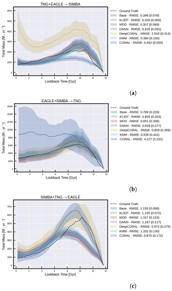
Figure A3.
Global SFH predictions for the three experiments. The curves correspond to the sums over all SFHs or predicted SFHs. (a) is when we train on eagle and illustrisTNG, and test on simba; (b) is when we train on eagle and simba, and test on illustrisTNG; (c) is when we train on simba and illustrisTNG, and test on eagle.
Appendix D. Predictions for Individual SFHs
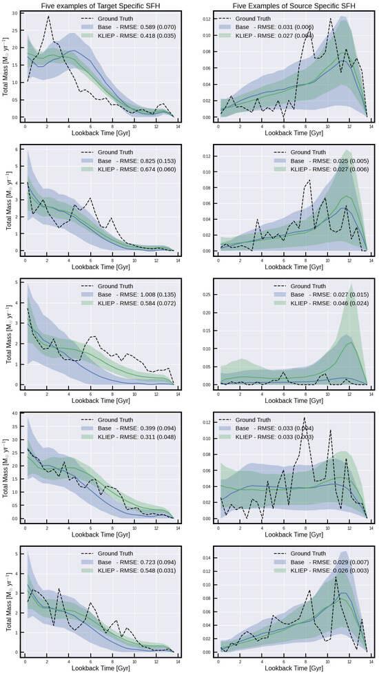
Figure A4.
Individuals galaxies for Simba from target- and source-specific clusters.
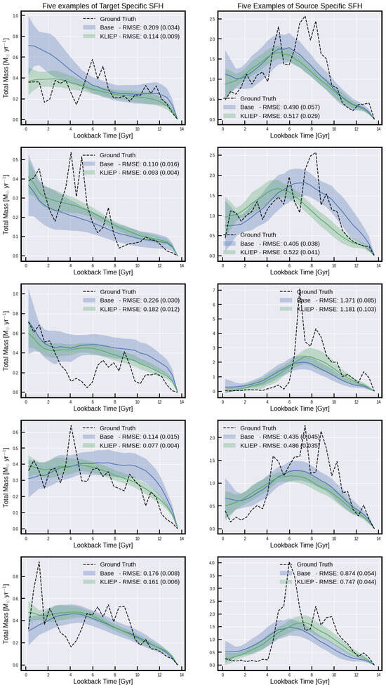
Figure A5.
Individuals galaxies for IllustrisTNG from target- and source-specific clusters.
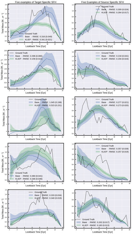
Figure A6.
Individuals galaxies for Eagle from target- and source-specific clusters.
Notes
| 1 | The observed CSFRD (especially at ) is still a topic of active research currently, as the amount of star formation obscured by dust in the early universe is still unknown. |
| 2 | A representative sampling looks like this: (0.0, 0.48), (0.48, 0.95), (0.95, 1.43), (1.43, 1.91), (1.91, 2.38), (2.38, 2.86), (2.86, 3.34), (3.34, 3.81), (3.81, 4.29), (4.29, 4.77), (4.77, 5.24), (5.24, 5.72), (5.72, 6.2), (6.2, 6.67), (6.67, 7.15), (7.15, 7.63), (7.63, 8.1), (8.1, 8.58), (8.58, 9.05), (9.05, 9.53), (9.53, 10.01), (10.01, 10.48), (10.48, 10.96), (10.96, 11.44), (11.44, 11.91), (11.91, 12.39), (12.39, 12.87), (12.87, 13.34), (13.34, 13.82), where all the values are in gigayears (GYrs). |
| 3 | https://github.com/antoinedemathelin/adapt (accessed on 6 April 2024). |
References
- Dai, W.; Yang, Q.; Xue, G.R.; Yu, Y. Boosting for Transfer Learning. In Proceedings of the 24th International Conference on Machine Learning, Vienna, Austria, 21–27 July 2007; Volume 227, pp. 193–200. [Google Scholar] [CrossRef]
- de Mathelin, A.; Richard, G.; Mougeot, M.; Vayatis, N. Adversarial weighting for domain adaptation in regression. arXiv 2020, arXiv:2006.08251. [Google Scholar]
- Motiian, S.; Jones, Q.; Iranmanesh, S.M.; Doretto, G. Few-Shot Adversarial Domain Adaptation. In Proceedings of the 31st International Conference on Neural Information Processing Systems, Red Hook, NY, USA, 4–9 December 2017; pp. 6673–6683. [Google Scholar]
- Motiian, S.; Piccirilli, M.; Adjeroh, D.A.; Doretto, G. Unified deep supervised domain adaptation and generalization. In Proceedings of the IEEE International Conference on Computer Vision, Venice, Italy, 22–29 October 2017; pp. 5715–5725. [Google Scholar]
- Liu, J.; Xuan, W.; Gan, Y.; Zhan, Y.; Liu, J.; Du, B. An End-to-end Supervised Domain Adaptation Framework for Cross-Domain Change Detection. Pattern Recognit. 2022, 132, 108960. [Google Scholar] [CrossRef]
- Hedegaard, L.; Sheikh-Omar, O.A.; Iosifidis, A. Supervised domain adaptation: A graph embedding perspective and a rectified experimental protocol. IEEE Trans. Image Process. 2021, 30, 8619–8631. [Google Scholar] [CrossRef]
- Kumar, A.; Saha, A.; Daume, H. Co-regularization based semi-supervised domain adaptation. Adv. Neural Inf. Process. Syst. 2010, 23, 478–486. [Google Scholar]
- Saito, K.; Kim, D.; Sclaroff, S.; Darrell, T.; Saenko, K. Semi-Supervised Domain Adaptation via Minimax Entropy. In Proceedings of the 2019 IEEE/CVF International Conference on Computer Vision (ICCV), Seoul, Republic of Korea, 27 October–2 November 2019; pp. 8049–8057. [Google Scholar]
- Tzeng, E.; Hoffman, J.; Darrell, T.; Saenko, K. Simultaneous Deep Transfer Across Domains and Tasks. In Proceedings of the 2015 IEEE International Conference on Computer Vision (ICCV), Santiago, Chile, 7–13 December 2015; pp. 4068–4076. [Google Scholar]
- Daumé, H., III; Kumar, A.; Saha, A. Frustratingly easy semi-supervised domain adaptation. In Proceedings of the 2010 Workshop on Domain Adaptation for Natural Language Processing, Uppsala, Sweden, 15 July 2010; pp. 53–59. [Google Scholar]
- Li, K.; Liu, C.; Zhao, H.; Zhang, Y.; Fu, Y. Ecacl: A holistic framework for semi-supervised domain adaptation. In Proceedings of the IEEE/CVF International Conference on Computer Vision, Virtual, 11–17 October 2021; pp. 8578–8587. [Google Scholar]
- Zhou, K.; Ziwei, L.; Yu, Q.; Xiang, T.; Loy, C.C. Domain Generalization: A Survey. IEEE Trans. Pattern Anal. Mach. Intell. 2023, 45, 4396–4415. [Google Scholar] [CrossRef]
- Huang, J.; Gretton, A.; Borgwardt, K.; Schölkopf, B.; Smola, A.J. Correcting Sample Selection Bias by Unlabeled Data. In Advances in Neural Information Processing Systems 19; Schölkopf, B., Platt, J.C., Hoffman, T., Eds.; MIT Press: Cambridge, MA, USA, 2007; pp. 601–608. [Google Scholar]
- Richard, G.; de Mathelin, A.; Hébrail, G.; Mougeot, M.; Vayatis, N. Unsupervised Multi-source Domain Adaptation for Regression. In Lecture Notes in Computer Science, Proceedings of the Machine Learning and Knowledge Discovery in Databases—European Conference, ECML PKDD 2020, Ghent, Belgium, 14–18 September 2020; Proceedings, Part I; Springer: Berlin/Heidelberg, Germany, 2020; Volume 12457, pp. 395–411. [Google Scholar]
- Saito, K.; Watanabe, K.; Ushiku, Y.; Harada, T. Maximum classifier discrepancy for unsupervised domain adaptation. In Proceedings of the IEEE Conference on Computer Vision and Pattern Recognition, Salt Lake City, UT, USA, 18–23 June 2018; pp. 3723–3732. [Google Scholar]
- Sugiyama, M.; Nakajima, S.; Kashima, H.; Bünau, P.v.; Kawanabe, M. Direct Importance Estimation with Model Selection and Its Application to Covariate Shift Adaptation. In Proceedings of the 20th International Conference on Neural Information Processing Systems, NIPS’07, Red Hook, NY, USA, 3–6 December 2007; pp. 1433–1440. [Google Scholar]
- Cortes, C.; Mohri, M.; Medina, A.M.n. Adaptation Based on Generalized Discrepancy. J. Mach. Learn. Res. 2019, 20, 1–30. [Google Scholar]
- Robotham, A.S.G.; Bellstedt, S.; Lagos, C.d.P.; Thorne, J.E.; Davies, L.J.; Driver, S.P.; Bravo, M. ProSpect: Generating spectral energy distributions with complex star formation and metallicity histories. Mon. Not. R. Astron. Soc. 2020, 495, 905–931. [Google Scholar] [CrossRef]
- da Cunha, E.; Charlot, S.; Elbaz, D. A simple model to interpret the ultraviolet, optical and infrared emission from galaxies. Mon. Not. R. Astron. Soc. 2008, 388, 1595–1617. [Google Scholar] [CrossRef]
- Da Cunha, E.; Charlot, S.; Dunne, L.; Smith, D.; Rowlands, K. MAGPHYS: A publicly available tool to interpret observed galaxy SEDs. Proc. Int. Astron. Union 2011, 7, 292–296. [Google Scholar] [CrossRef]
- Noll, S.; Burgarella, D.; Giovannoli, E.; Buat, V.; Marcillac, D.; Muñoz-Mateos, J.C. Analysis of galaxy spectral energy distributions from far-UV to far-IR with CIGALE: Studying a SINGS test sample. Astron. Astrophys. 2009, 507, 1793–1813. [Google Scholar] [CrossRef]
- Boquien, M.; Burgarella, D.; Roehlly, Y.; Buat, V.; Ciesla, L.; Corre, D.; Inoue, A.K.; Salas, H. CIGALE: A Python code investigating galaxy emission. Astron. Astrophys. 2019, 622, A103. [Google Scholar] [CrossRef]
- Carnall, A.C.; McLure, R.J.; Dunlop, J.S.; Davé, R. Inferring the star formation histories of massive quiescent galaxies with BAGPIPES: Evidence for multiple quenching mechanisms. Mon. Not. R. Astron. Soc. 2018, 480, 4379–4401. [Google Scholar] [CrossRef]
- Crocker, D.L.; French, K.D.; Tripathi, A.; Verrico, M.E. Modeling Star Formation Histories of Post Starburst Galaxies with BAGPIPES. Res. Notes AAS 2023, 7, 183. [Google Scholar] [CrossRef]
- Johnson, B.; Leja, J. Bd-J/Prospector: Initial Release; Zenodo: Geneva, Switzerland, 2017. [Google Scholar] [CrossRef]
- Johnson, B.D.; Leja, J.; Conroy, C.; Speagle, J.S. Stellar population inference with Prospector. Astrophys. J. Suppl. Ser. 2021, 254, 22. [Google Scholar] [CrossRef]
- Dattilo, A.; Vanderburg, A.; Shallue, C.J.; Mayo, A.W.; Berlind, P.; Bieryla, A.; Calkins, M.; Esquerdo, G.A.; Everett, M.E.; Howell, S.B.; et al. Identifying exoplanets with deep learning. ii. Two new super-earths uncovered by a neural network in K2 data. Astron. J. 2019, 157, 169. [Google Scholar] [CrossRef]
- Jara-Maldonado, M.; Alarcon-Aquino, V.; Rosas-Romero, R.; Starostenko, O.; Ramirez-Cortes, J.M. Transiting exoplanet discovery using machine learning techniques: A survey. Earth Sci. Inform. 2020, 13, 573–600. [Google Scholar] [CrossRef]
- Zucker, S.; Giryes, R. Shallow transits—Deep learning. I. Feasibility study of deep learning to detect periodic transits of exoplanets. Astron. J. 2018, 155, 147. [Google Scholar] [CrossRef]
- Caldeira, J.; Wu, W.K.; Nord, B.; Avestruz, C.; Trivedi, S.; Story, K.T. DeepCMB: Lensing reconstruction of the cosmic microwave background with deep neural networks. Astron. Comput. 2019, 28, 100307. [Google Scholar] [CrossRef]
- Escamilla-Rivera, C.; Carvajal, M.A.; Capozziello, S. A deep learning approach to cosmological dark energy models. J. Cosmol. Astropart. Phys. 2020, 2020, 8. [Google Scholar] [CrossRef]
- Hortúa, H.J.; Volpi, R.; Marinelli, D.; Malagò, L. Parameter estimation for the cosmic microwave background with Bayesian neural networks. Phys. Rev. D 2020, 102, 103509. [Google Scholar] [CrossRef]
- Cuoco, E.; Powell, J.; Cavaglià, M.; Ackley, K.; Bejger, M.; Chatterjee, C.; Coughlin, M.; Coughlin, S.; Easter, P.; Essick, R.; et al. Enhancing gravitational-wave science with machine learning. Mach. Learn. Sci. Technol. 2020, 2, 011002. [Google Scholar] [CrossRef]
- Bayley, J.; Messenger, C.; Woan, G. Robust machine learning algorithm to search for continuous gravitational waves. Phys. Rev. D 2020, 102, 083024. [Google Scholar] [CrossRef]
- Schäfer, M.B.; Ohme, F.; Nitz, A.H. Detection of gravitational-wave signals from binary neutron star mergers using machine learning. Phys. Rev. D 2020, 102, 063015. [Google Scholar] [CrossRef]
- Cavanagh, M.K.; Bekki, K.; Groves, B.A. Morphological classification of galaxies with deep learning: Comparing 3-way and 4-way CNNs. Mon. Not. R. Astron. Soc. 2021, 506, 659–676. [Google Scholar] [CrossRef]
- Barchi, P.H.; de Carvalho, R.R.; Rosa, R.R.; Sautter, R.A.; Soares-Santos, M.; Marques, B.A.D.; Clua, E.; Gonçalves, T.S.; de Sá-Freitas, C.; Moura, T.C. Machine and Deep Learning applied to galaxy morphology—A comparative study. Astron. Comput. 2020, 30, 100334. [Google Scholar] [CrossRef]
- D’Isanto, A.; Polsterer, K.L. Photometric redshift estimation via deep learning-generalized and pre-classification-less, image based, fully probabilistic redshifts. Astron. Astrophys. 2018, 609, A111. [Google Scholar] [CrossRef]
- Hoyle, B. Measuring photometric redshifts using galaxy images and Deep Neural Networks. Astron. Comput. 2016, 16, 34–40. [Google Scholar] [CrossRef]
- Gilda, S.; Ting, Y.-S.; Withington, K.; Wilson, M.; Prunet, S.; Mahoney, W.; Fabbro, S.; Draper, S.C.; Sheinis, A. Astronomical Image Quality Prediction based on Environmental and Telescope Operating Conditions. arXiv 2020, arXiv:2011.03132. [Google Scholar]
- Gilda, S.; Draper, S.C.; Fabbro, S.; Mahoney, W.; Prunet, S.; Withington, K.; Wilson, M.; Ting, Y.-S.; Sheinis, A. Uncertainty-aware learning for improvements in image quality of the Canada–France–Hawaii Telescope. Mon. Not. R. Astron. Soc. 2022, 510, 870–902. [Google Scholar] [CrossRef]
- Dainotti, M.; Petrosian, V.; Bogdan, M.; Miasojedow, B.; Nagataki, S.; Hastie, T.; Nuyngen, Z.; Gilda, S.; Hernandez, X.; Krol, D. Gamma-ray Bursts as distance indicators through a machine learning approach. arXiv 2019, arXiv:1907.05074. [Google Scholar]
- Ukwatta, T.N.; Woźniak, P.R.; Gehrels, N. Machine-z: Rapid machine-learned redshift indicator for Swift gamma-ray bursts. Mon. Not. R. Astron. Soc. 2016, 458, 3821–3829. [Google Scholar] [CrossRef]
- Gilda, S. deep-REMAP: Parameterization of Stellar Spectra Using Regularized Multi-Task Learning. arXiv 2023, arXiv:2311.03738. [Google Scholar]
- Ramachandra, N.; Chaves-Montero, J.; Alarcon, A.; Fadikar, A.; Habib, S.; Heitmann, K. Machine learning synthetic spectra for probabilistic redshift estimation: SYTH-Z. Mon. Not. R. Astron. Soc. 2022, 515, 1927–1941. [Google Scholar] [CrossRef]
- Gilda, S.; Lower, S.; Narayanan, D. mirkwood: Fast and Accurate SED Modeling Using Machine Learning. Astrophys. J. 2021, 916, 43. [Google Scholar] [CrossRef]
- Gilda, S. Beyond mirkwood: Enhancing SED Modeling with Conformal Predictions. Astronomy 2024, 3, 14–20. [Google Scholar] [CrossRef]
- Schaye, J.; Crain, R.A.; Bower, R.G.; Furlong, M.; Schaller, M.; Theuns, T.; Dalla Vecchia, C.; Frenk, C.S.; McCarthy, I.G.; Helly, J.C.; et al. The EAGLE project: Simulating the evolution and assembly of galaxies and their environments. Mon. Not. R. Astron. Soc. 2015, 446, 521–554. [Google Scholar] [CrossRef]
- Nelson, D.; Pillepich, A.; Springel, V.; Weinberger, R.; Hernquist, L.; Pakmor, R.; Genel, S.; Torrey, P.; Vogelsberger, M.; Kauffmann, G.; et al. First results from the IllustrisTNG simulations: The galaxy colour bimodality. Mon. Not. R. Astron. Soc. 2018, 475, 624–647. [Google Scholar] [CrossRef]
- Pillepich, A.; Nelson, D.; Hernquist, L.; Springel, V.; Pakmor, R.; Torrey, P.; Weinberger, R.; Genel, S.; Naiman, J.P.; Marinacci, F.; et al. First results from the IllustrisTNG simulations: The stellar mass content of groups and clusters of galaxies. Mon. Not. R. Astron. Soc. 2018, 475, 648–675. [Google Scholar] [CrossRef]
- Davé, R.; Anglés-Alcázar, D.; Narayanan, D.; Li, Q.; Rafieferantsoa, M.H.; Appleby, S. SIMBA: Cosmological simulations with black hole growth and feedback. Mon. Not. R. Astron. Soc. 2019, 486, 2827–2849. [Google Scholar] [CrossRef]
- Schaller, M.; Dalla Vecchia, C.; Schaye, J.; Bower, R.G.; Theuns, T.; Crain, R.A.; Furlong, M.; McCarthy, I.G. The EAGLE simulations of galaxy formation: The importance of the hydrodynamics scheme. Mon. Not. R. Astron. Soc. 2015, 454, 2277–2291. [Google Scholar] [CrossRef]
- McAlpine, S.; Helly, J.C.; Schaller, M.; Trayford, J.W.; Qu, Y.; Furlong, M.; Bower, R.G.; Crain, R.A.; Schaye, J.; Theuns, T.; et al. The EAGLE simulations of galaxy formation: Public release of halo and galaxy catalogues. Astron. Comput. 2016, 15, 72–89. [Google Scholar] [CrossRef]
- Vogelsberger, M.; Genel, S.; Springel, V.; Torrey, P.; Sijacki, D.; Xu, D.; Snyder, G.; Nelson, D.; Hernquist, L. Introducing the Illustris Project: Simulating the coevolution of dark and visible matter in the Universe. Mon. Not. R. Astron. Soc. 2014, 444, 1518–1547. [Google Scholar] [CrossRef]
- Madau, P.; Dickinson, M. Cosmic Star-Formation History. Annu. Rev. Astron. Astrophys. 2014, 52, 415–486. [Google Scholar] [CrossRef]
- Schölkopf, B.; Burges, C.J.; Smola, A.J. (Eds.) Advances in Kernel Methods: Support Vector Learning; MIT Press: Cambridge, MA, USA, 1999. [Google Scholar]
- Mika, S.; Schölkopf, B.; Smola, A.; Müller, K.-R.; Scholz, M.; Rätsch, G. Kernel PCA and de-noising in feature spaces. Adv. Neural Inf. Process. Syst. 1998, 11. [Google Scholar]
- Jolliffe, I.T.; Cadima, J. Principal component analysis: A review and recent developments. Philos. Trans. R. Soc. Lond. Ser. A 2016, 374, 20150202. [Google Scholar] [CrossRef]
- Greenacre, M.; Groenen, P.J.F.; Hastie, T.; d’Enza, A.I.; Markos, A.; Tuzhilina, E. Principal component analysis. Nat. Rev. Methods Prim. 2022, 2, 100. [Google Scholar] [CrossRef]
- Shensa, M.J. The discrete wavelet transform: Wedding the a trous and Mallat algorithms. IEEE Trans. Signal Process. 1992, 40, 2464–2482. [Google Scholar] [CrossRef]
- Heil, C.E.; Walnut, D.F. Continuous and discrete wavelet transforms. SIAM Rev. 1989, 31, 628–666. [Google Scholar] [CrossRef]
- Le Guen, V.; Thome, N. Deep Time Series Forecasting With Shape and Temporal Criteria. IEEE Trans. Pattern Anal. Mach. Intell. 2023, 45, 342–355. [Google Scholar] [CrossRef]
- Cortes, C.; Mohri, M. Domain adaptation and sample bias correction theory and algorithm for regression. Theor. Comput. Sci. 2014, 519, 103–126. [Google Scholar] [CrossRef]
- Mansour, Y.; Mohri, M.; Rostamizadeh, A. Domain Adaptation: Learning Bounds and Algorithms. In Proceedings of the 22nd Annual Conference on Learning Theory (COLT 2009), Montreal, QC, Canada, 18–21 June 2009. [Google Scholar]
- Kingma, D.P.; Ba, J. Adam: A Method for Stochastic Optimization. In Proceedings of the 3rd International Conference on Learning Representations, ICLR 2015, San Diego, CA, USA, 7–9 May 2015; Conference Track Proceedings. Bengio, Y., LeCun, Y., Eds.; ArXiv: Ithaca, NY, USA, 2015. [Google Scholar]
- Bellstedt, S.; Robotham, A.S.G.; Driver, S.P.; Thorne, J.E.; Davies, L.J.M.; Lagos, C.d.P.; Stevens, A.R.H.; Taylor, E.N.; Baldry, I.K.; Moffett, A.J.; et al. Galaxy And Mass Assembly (GAMA): A forensic SED reconstruction of the cosmic star formation history and metallicity evolution by galaxy type. Mon. Not. R. Astron. Soc. 2020, 498, 5581–5603. [Google Scholar] [CrossRef]
- Lagos, C.d.P.; Tobar, R.J.; Robotham, A.S.G.; Obreschkow, D.; Mitchell, P.D.; Power, C.; Elahi, P.J. Shark: Introducing an open source, free, and flexible semi-analytic model of galaxy formation. Mon. Not. R. Astron. Soc. 2018, 481, 3573–3603. [Google Scholar] [CrossRef]
- Zhang, Y.; Liu, T.; Long, M.; Jordan, M. Bridging theory and algorithm for domain adaptation. In Proceedings of the 36th International Conference on Machine Learning, Long Beach, CA, USA, 9–15 June 2019; pp. 7404–7413. [Google Scholar]
- Ganin, Y.; Ustinova, E.; Ajakan, H.; Germain, P.; Larochelle, H.; Laviolette, F.; March, M.; Lempitsky, V. Domain-adversarial training of neural networks. J. Mach. Learn. Res. 2016, 17, 2096–2130. [Google Scholar]
- Huang, J.; Smola, A.; Gretton, A.; Borgwardt, K.; Scholkopf, B. Correcting sample selection bias by unlabeled data. In Proceedings of the 19th International Conference on Neural Information Processing Systems, Vancouver, BC, Canada, 4–9 December 2006; pp. 601–608. [Google Scholar]
- Sun, B.; Feng, J.; Saenko, K. Return of frustratingly easy domain adaptation. In Proceedings of the AAAI Conference on Artificial Intelligence, Phoenix, AZ, USA, 12–17 February 2016; Volume 30. No. 1. [Google Scholar]
- Sun, B.; Saenko, K. Deep coral: Correlation alignment for deep domain adaptation. In Proceedings of the Computer Vision–ECCV 2016 Workshops, Amsterdam, The Netherlands, 11–14 October 2016; Proceedings, Part III 14. pp. 443–450. [Google Scholar]
- Zhao, H.; Zhang, S.; Wu, G.; Moura, J.M.F.; Costeira, J.P.; Gordon, G.J. Adversarial Multiple Source Domain Adaptation. In Proceedings of the Advances in Neural Information Processing Systems 31, Montreal, QC, Canada, 3–8 December 2018; Bengio, S., Wallach, H., Larochelle, H., Grauman, K., Cesa-Bianchi, N., Garnett, R., Eds.; Curran Associates, Inc.: Nice, France, 2018; pp. 8559–8570. [Google Scholar]
- Richard, G.; Mathelin, A.; Hébrail, G.; Mougeot, M.; Vayatis, N. Unsupervised Multi-source Domain Adaptation for Regression. In Proceedings of the European Conference, ECML PKDD 2020, Ghent, Belgium, 14–18 September 2020. pp. 395–411. [CrossRef]
- Salpeter, E.E. The Luminosity Function and Stellar Evolution. Astrophys. J. 1955, 121, 161. [Google Scholar] [CrossRef]
- Kroupa, P. On the variation of the initial mass function. Mon. Not. R. Astron. Soc. 2001, 322, 231–246. [Google Scholar] [CrossRef]
- Chabrier, G. Galactic Stellar and Substellar Initial Mass Function. Publ. Astron. Soc. Pac. 2003, 115, 763–795. [Google Scholar] [CrossRef]
- Bruzual, G.; Charlot, S. Stellar population synthesis at the resolution of 2003. Mon. Not. R. Astron. Soc. 2003, 344, 1000–1028. [Google Scholar] [CrossRef]
- Tremonti, C.A.; Heckman, T.M.; Kauffmann, G.; Brinchmann, J.; Charlot, S.; White, S.D.M.; Seibert, M.; Peng, E.W.; Schlegel, D.J.; Uomoto, A.; et al. The Origin of the Mass-Metallicity Relation: Insights from 53,000 Star-forming Galaxies in the Sloan Digital Sky Survey. Astrophys. J. 2004, 613, 898–913. [Google Scholar] [CrossRef]
- Jimmy; Tran, K.V.; Saintonge, A.; Accurso, G.; Brough, S.; Oliva-Altamirano, P. The Gas Phase Mass Metallicity Relation for Dwarf Galaxies: Dependence on Star Formation Rate and HI Gas Mass. Astrophys. J. 2015, 812, 98. [Google Scholar] [CrossRef]
- Lara-Lopez, M.A.; Hopkins, A.M.; Lopez-Sanchez, A.R.; Brough, S.; Colless, M.; Bland-Hawthorn, J.; Driver, S.; Foster, C.; Liske, J.; Loveday, J.; et al. Galaxy and mass assembly (GAMA): The connection between metals, specific SFR and hi gas in galaxies: The Z-SSFR relation. Mon. Not. R. Astron. Soc. 2013, 433, L35–L39. [Google Scholar] [CrossRef]
Disclaimer/Publisher’s Note: The statements, opinions and data contained in all publications are solely those of the individual author(s) and contributor(s) and not of MDPI and/or the editor(s). MDPI and/or the editor(s) disclaim responsibility for any injury to people or property resulting from any ideas, methods, instructions or products referred to in the content. |
© 2024 by the authors. Licensee MDPI, Basel, Switzerland. This article is an open access article distributed under the terms and conditions of the Creative Commons Attribution (CC BY) license (https://creativecommons.org/licenses/by/4.0/).