On the Dynamical Instability of Monatomic Fluid Spheres in (N + 1)-Dimensional Spacetime

Abstract

In this note, I derive the Chandrasekhar instability of a fluid sphere in (N + 1)-dimensional Schwarzschild–Tangherlini spacetime and take the homogeneous (uniform energy density) solution for illustration. Qualitatively, the effect of a positive (negative) cosmological constant tends to destabilize (stabilize) the sphere. In the absence of a cosmological constant, the privileged position of (3 + 1)-dimensional spacetime is manifest in its own right. As it is, the marginal dimensionality in which a monatomic ideal fluid sphere is stable but not too stable to trigger the onset of gravitational collapse. Furthermore, it is the unique dimensionality that can accommodate stable hydrostatic equilibrium with a positive cosmological constant. However, given the current cosmological constant observed, no stable configuration can be larger than ${10}^{21}{\mathrm{M}}_{\odot }$. On the other hand, in (2 + 1) dimensions, it is too stable either in the context of Newtonian Gravity (NG) or Einstein’s General Relativity (GR). In GR, the role of negative cosmological constant is crucial not only to guarantee fluid equilibrium (decreasing monotonicity of pressure) but also to have the Bañados–Teitelboim–Zanelli (BTZ) black hole solution. Owing to the negativeness of the cosmological constant, there is no unstable configuration for a homogeneous fluid disk with mass $0<\mathcal{M}\le 0.5$ to collapse into a naked singularity, which supports the Cosmic Censorship Conjecture. However, the relativistic instability can be triggered for a homogeneous disk with mass $0.5<\mathcal{M}\lesssim 0.518$ under causal limit, which implies that BTZ holes of mass ${\mathcal{M}}_{\mathrm{BTZ}}>0$ could emerge from collapsing fluid disks under proper conditions. The implicit assumptions and implications are also discussed.

1. Introduction

Dimensionality of spacetime is a question with a long history [1,2,3,4,5,6,7,8]. Starting from Ehrenfest [1,2], who argued based on the “stability postulate” of the two-body problem, the fundamental laws of physics favor (3 + 1) dimensions. His approach is still valid in the framework of general relativity (GR) as well as hydrogen atoms, as was shown by Tangherlini [4]; however, see Ref. [7] for an alternative procedure and references therein. Tegmark [8] argued that the existence of only one temporal dimension by requiring hyperbolic equations of motion, and hence predictability, leaves the question why three (macroscopic) spatial dimensions are favorable. Various arguments were proposed for the reasoning [9,10,11,12,13,14,15], although the dimensionality could be dynamical and scale-dependent, as a physical observable [16].

Presumably, the “non-compact” (3 + 1) dimensions might be just an illusion due to our human perception. However, constraint from gravitational waves indicates that we certainly live in a universe of non-compact (3 + 1) dimensions [17], as described by GR. On the other hand, although it was usually cited that structures in (2 + 1) are not complex enough to accommodate life, as opposed to the common view, life that could exist in (2 + 1) was discussed more recently [18].

Stellar equilibrium in different dimensions has also been explored previously [19,20,21]. One important feature on stellar stability in GR is the Buchdahl stability bound [22]. It states that the mass of a spherical compact object must exceed the $9/4$ of its gravitational radius in (3 + 1) dimensions. Otherwise, there is no stable stellar equilibrium, and it would definitely collapse into a black hole. Buchdahl bound in higher dimensions [19] with cosmological constant [21] and its universality in other gravity theories [23,24,25] were also investigated previously. Nonetheless, the dynamical instability of a star might have set in well before the Buchdahl bound.

The dynamical instability of a self-gravitating sphere in the context of GR has been explored long ago by Chandrasekhar (1964) [26,27] and Zel’dovich and Podurets (1966) [28], via the study of a pulsation equation and binding energy, respectively. It was found that the turning point of fractional binding energy [29,30] is very close to the result using the pulsation equation [31]. Chandrasekhar’s criterion [26,27] provides a sufficient condition triggering the black hole formation. In hydrostatic equilibrium, the pressure of a star balances its self-gravity. As a gravitationally bound system, a star behaves as if it has negative specific heat: The more energy it loses, the hotter it becomes [32,33]. Therefore, it undergoes the gravothermal evolution due to the heat dissipations. At each evolution stage, the instability might set in depending on the fluid’s stiffness, which is characterized by its adiabatic index [31]. For example, the adiabatic index of a (3 + 1) monatomic ideal fluid transitions from $5/3$ (stiff) toward $4/3$ (soft) when the particles become more relativistic through the conversion of gravitational energy. This method has also been extended to address the stellar instability in (3 + 1) spacetime with a non-zero cosmological constant [34,35], the extra dimension influence [36] on the strange quark stars, the stability of supermassive stars [37], and the self-interacting dark halo core collapse [31,38]. However, see also the gravothermal instabilities from energy consideration in [39,40,41].

In (2 + 1) spacetime, a negative cosmological constant is to guarantee not only hydrostatic equilibrium [42] (the pressure is monotonically decreasing) but also permit a black hole solution of Bañados–Teitelboim–Zanelli (BTZ) [43]. The dynamical process of dust collapse [44], critical collapse of scalar field [45,46,47], and ultra-relativistic fluid [48,49] into a BTZ hole have been shown to be possible. Nevertheless, in this note, we are more interested in the condition triggering the dynamical instability of a monatomic fluid disk in the hydrodynamic limit. The pressure in a fluid can not be ignored because it could prevent the fluid from further collapse. On the other hand, as the random motion of the particles in the fluid influences the gravitational potential in the macroscopic picture through the pressure effect, (2 + 1) static stars of perfect fluid qualitatively differ in their behavior from that of dust [50]. As a result, rather than counteract the gravitational attraction, it could further destabilize the fluid disk at some point, just as the cases of (3 + 1). However, the negative cosmological constant introduced tends to stabilize the fluid. Thus, the competition between the pressure (relativistic) effect and the cosmological constant is crucial to trigger the black hole formation.

In this work, we examine the space dimensionality N from the viewpoint of the Chandrasekhar instability of an ideal monatomic fluid sphere in (N + 1) dimensions. The paper is organized as follows: We first derive the (N + 1) pulsation equation of a perfect fluid sphere with and without cosmological constant and the corresponding Chandrasekhar’s criterion in Section 2. As an illustration, we then present the (N + 1) homogeneous (uniform energy density) solution in Section 3 and numerically determine the condition at the onset of instabilities in Section 4. We briefly summarize the results with the implicit assumptions, and discuss the physical implications in Section 5. In particular, we assume that GR equations hold, the fluid sphere is homogeneous and monatomic. Geometric unit ($G_N=c=1$) is used throughout the text, where $G_N$ is the Newton’s constant in (N + 1) dimensions.

2. (N + 1)-Dimensional Spacetime of Spherical Symmetry

We consider a spherically symmetric spacetime in (N + 1) dimensions,

$$\mathrm{d}{s}^2=-e^{2\mathsf{\Phi }(t,r)}\mathrm{d}{t}^2+e^{2\mathsf{\Lambda }(t,r)}\mathrm{d}{r}^2+r^2\mathrm{d}{\mathsf{\Omega }}_{N-1}^2,$$

(1)

where

$$\mathrm{d}{\mathsf{\Omega }}_{N-1}^2=\mathrm{d}{\theta }_1^2+{sin}^2{\theta }_1\mathrm{d}{\theta }_2^2+\dots +\prod _{j=1}^{N-2}{sin}^2{\theta }_j\mathrm{d}{\theta }_{N-1}^2.$$

(2)

After the standard calculations, the field equations $G^{\mu }{}_{\nu }={\kappa }_N{T}^{\mu }{}_{\nu }$ give

$$-\frac{(N-1){\mathsf{\Lambda }}^{\prime }}{r}{e}^{-2\mathsf{\Lambda }}-\frac{(N-1)(N-2)}{2r^2}\left[1-e^{-2\mathsf{\Lambda }}\right]={\kappa }_N{T}^t{}_t,$$

(3a)

$$\frac{(N-1)\mathsf{\Phi }{}^{\prime }}{r}{e}^{-2\mathsf{\Lambda }}-\frac{(N-1)(N-2)}{2r^2}\left[1-e^{-2\mathsf{\Lambda }}\right]={\kappa }_N{T}^r{}_r,$$

(3b)

$$\frac{N-1}{r}\dot{\mathsf{\Lambda }}{e}^{-2\mathsf{\Lambda }}={\kappa }_N{T}^r{}_t,$$

(3c)

$$\begin{array}{cc}\hfill & \left[\mathsf{\Phi }{}^{″}+\mathsf{\Phi }{{}^{\prime }}^2-\mathsf{\Phi }{}^{\prime }\mathsf{\Lambda }{}^{\prime }+\frac{(N-2)}{r}(\mathsf{\Phi }{}^{\prime }-\mathsf{\Lambda }{}^{\prime })\right]e^{-2\mathsf{\Lambda }}\hfill \\ \hfill & -\frac{(N-2)(N-3)}{2r^2}\left[1-e^{-2\mathsf{\Lambda }}\right]-(\ddot{\mathsf{\Lambda }}+{\dot{\mathsf{\Lambda }}}^2-\dot{\mathsf{\Phi }}\dot{\mathsf{\Lambda }})e^{-2\mathsf{\Phi }}={\kappa }_N{T}^{{\theta }_1}{}_{{\theta }_1},\hfill \end{array}$$

(3d)

where the “prime” and “dot” denote the “radial” and “time” derivatives, respectively, and $T^{{\theta }_1}{}_{{\theta }_1}=T^{{\theta }_2}{}_{{\theta }_2}=\dots =T^{{\theta }_{N-1}}{}_{{\theta }_{N-1}}\equiv p$ because of spherical symmetry. On the other hand, combining Equations (3a) and (3b), we obtain

$$\frac{(N-1)}{r}(\mathsf{\Phi }{}^{\prime }+\mathsf{\Lambda }{}^{\prime })e^{-2\mathsf{\Lambda }}={\kappa }_N(T^r{}_r-T^t{}_t).$$

(4)

The conservation of energy–momentum tensor ${\nabla }_{\mu }{T}^{\mu }{}_{\nu }=0$ leads to

$${\partial }_t{T}^t{}_t+{\partial }_r{T}^r{}_t+(T^t{}_t-T^r{}_r)\dot{\mathsf{\Lambda }}+T^r{}_t\left(\mathsf{\Phi }{}^{\prime }+\mathsf{\Lambda }{}^{\prime }+\frac{N-1}{r}\right)=0$$

(5a)

and

$${\partial }_t{T}^t{}_r+{\partial }_r{T}^r{}_r+T^t{}_r(\dot{\mathsf{\Phi }}+\dot{\mathsf{\Lambda }})+(T^r{}_r-T^t{}_t)\mathsf{\Phi }{}^{\prime }+\frac{N-1}{r}(T^r{}_r-p)=0.$$

(5b)

If we define the Schwarzschild mass function $M\left(r\right)$ through

$$1-e^{-2\mathsf{\Lambda }}\equiv 2M/r^{N-2},$$

(6)

then $G^t{}_t={\kappa }_N{T}^t{}_t=-{\kappa }_N\rho$ leads to $M^{\prime }\left(r\right)=[{\kappa }_N/(N-1)]\rho r^{N-1}$. Accordingly, the mass function

$$M\left(r\right)={\omega }_N{\int }_0^r\rho {\overline{r}}^{N-1}d\overline{r},$$

(7)

where

$${\omega }_N=\frac{2{\pi }^{N/2}}{\mathsf{\Gamma }(N/2)}=\frac{{\kappa }_N}{N-1}$$

(8)

is the area of the unit sphere in N-dimensional space. Therefore, by construction, the Einstein coupling constant ${\kappa }_N=(N-1){\omega }_N$ automatically imposes the vacuum identity $G^{\mu }{}_{\nu }=0$ of Einsteinian gravity in (1 + 1) dimensions.

Now, we consider isotropic pressure ($T^r{}_r=p$) in static situation, Equation (5b) leads to $p^{\prime }=-(\rho +p){\mathsf{\Phi }}^{\prime }$, and ${\mathsf{\Phi }}^{\prime }$ can be replaced via Equation (3b), resulting in the Tolman–Oppenheimer–Volkoff (TOV) equation in (N + 1) dimensions:

$$\left(1-\frac{2M}{r^{N-2}}\right)p^{\prime }=-(\rho +p)\left(\frac{(N-2)M}{r^{N-1}}+\frac{{\kappa }_N}{N-1}pr\right).$$

(9)

Equation-of-state (EoS) $p=p\left(\rho \right)$ and boundary conditions $M\left(0\right)=0$, $p\left(R\right)=0$ must be imposed in order to determine the total fluid mass $\mathcal{M}\equiv M\left(R\right)$.

2.1. Linear Radial Perturbation and the Adiabatic Index

The perfect fluid description $T^{\mu }{}_{\nu }=(\rho +p)u^{\mu }{u}_{\nu }+p{\delta }^{\mu }{}_{\nu }$ implies $T^r{}_t=0$ in the static case. However, under the linear radial perturbation${\partial }_t\xi =\dot{\xi }\equiv dr/dt$,

$$T^r{}_t=-(\rho +p)\dot{\xi },$$

(10)

where $u^{\mu }$ is the 4-velocity of the fluid element, and we have introduced the “Lagrangian displacement” $\xi$ as well as $u_t=-e^{\mathsf{\Phi }}$, $u^r=e^{-\mathsf{\Phi }}\dot{\xi }$.

Now, we denote all the variables X’s in equilibrium by $X_0\left(r\right)$, which is independent of time. After perturbation $X(t,r)=X_0\left(r\right)+\delta X(t,r)$, only the perturbed quantities have the time dependence, where $\delta$ denotes the “Eulerian change” of the perturbation. Keeping only the terms of first-order corrections from Equations (3a), (3b), (3c), (5a) and (5b), we have the linearized equations governing the perturbation

$${\left[r^{N-2}{e}^{-2{\mathsf{\Lambda }}_0}2\delta \mathsf{\Lambda }\right]}^{\prime }=\frac{2{\kappa }_N}{N-1}{r}^{N-1}\delta \rho ,$$

(11a)

$$\frac{N-1}{r}{e}^{-2{\mathsf{\Lambda }}_0}(\delta \mathsf{\Phi }{}^{\prime }-2{\mathsf{\Phi }}_0{}^{\prime }\delta \mathsf{\Lambda })-\frac{(N-1)(N-2)}{r^2}{e}^{-2{\mathsf{\Lambda }}_0}\delta \mathsf{\Lambda }={\kappa }_N\delta p,$$

(11b)

$$\frac{N-1}{r}{e}^{-2{\mathsf{\Lambda }}_0}\delta \dot{\mathsf{\Lambda }}=-{\kappa }_N({\rho }_0+p_0)\dot{\xi }=-\frac{N-1}{r}{e}^{-2{\mathsf{\Lambda }}_0}({\mathsf{\Phi }}_0{}^{\prime }+{\mathsf{\Lambda }}_0{}^{\prime })\dot{\xi },$$

(11c)

$$\delta \dot{\rho }+{\left[({\rho }_0+p_0)\dot{\xi }\right]}^{\prime }+({\rho }_0+p_0)\left[\delta \dot{\mathsf{\Lambda }}+\dot{\xi }\left({\mathsf{\Phi }}_0^{\prime }+{\mathsf{\Lambda }}_0^{\prime }+\frac{N-1}{r}\right)\right]=0,$$

(11d)

$$e^{2({\mathsf{\Lambda }}_0-{\mathsf{\Phi }}_0)}({\rho }_0+p_0)\ddot{\xi }+\delta p^{\prime }+({\rho }_0+p_0)\delta \mathsf{\Phi }{}^{\prime }+(\delta \rho +\delta p){\mathsf{\Phi }}_0{}^{\prime }=0,$$

(11e)

respectively. In addition, Equation (10) also leads to

$$\delta \mathsf{\Lambda }=-\xi ({\mathsf{\Phi }}_0{}^{\prime }+{\mathsf{\Lambda }}_0{}^{\prime }),$$

(12)

thus Equations (11a) and (11d) (after performing time integration) identically lead to

$$\delta \rho =-\frac{1}{r^{N-1}}{\left[r^{N-1}({\rho }_0+p_0)\xi \right]}^{\prime }=-\xi \frac{\mathrm{d}{\rho }_0}{\mathrm{d}r}-\xi \frac{\mathrm{d}{p}_0}{\mathrm{d}r}-({\rho }_0+p_0)\frac{1}{r^{N-1}}{\left(r^{N-1}\xi \right)}^{\prime }$$

(13a)

or with the substitution $p_0^{\prime }=-({\rho }_0+p_0){\mathsf{\Phi }}_0{}^{\prime }$, we obtain

$$\Delta \rho =\delta \rho +\xi \frac{\mathrm{d}{\rho }_0}{\mathrm{d}r}=-({\rho }_0+p_0)\frac{e^{{\mathsf{\Phi }}_0}}{r^{N-1}}{\left(r^{N-1}{e}^{-{\mathsf{\Phi }}_0}\xi \right)}^{\prime },$$

(13b)

where $\Delta =\delta +\xi {\partial }_r$ denotes the “Lagrangian change” of the perturbation. To express $\delta p$ in terms of $\xi$, we assume the conservation of the baryon number ${\nabla }_{\alpha }\left(n{u}^{\alpha }\right)=0$, that is,

$${\partial }_t\left(n{e}^{-\mathsf{\Phi }}\right)+{\partial }_r\left(n\dot{\xi }{e}^{-\mathsf{\Phi }}\right)+n{e}^{-\mathsf{\Phi }}(\dot{\mathsf{\Phi }}+\dot{\mathsf{\Lambda }})+n{e}^{-\mathsf{\Phi }}\dot{\xi }\left(\mathsf{\Phi }{}^{\prime }+\mathsf{\Lambda }{}^{\prime }+\frac{N-1}{r}\right)=0.$$

(14)

Keeping only the first-order terms of perturbation, one obtains

$$e^{-{\mathsf{\Phi }}_0}\delta \dot{n}+\frac{1}{r^{N-1}}{\left(n_0{r}^{N-1}\dot{\xi }{e}^{-{\mathsf{\Phi }}_0}\right)}^{\prime }+n_0{e}^{-{\mathsf{\Phi }}_0}\delta \dot{\mathsf{\Lambda }}+n_0{e}^{-{\mathsf{\Phi }}_0}\dot{\xi }({\mathsf{\Phi }}_0{}^{\prime }+{\mathsf{\Lambda }}_0{}^{\prime })=0.$$

(15)

After integration over time and using Equation (12), reduce to

$$\delta n=-\frac{e^{{\mathsf{\Phi }}_0}}{r^{N-1}}{\left(n_0{r}^{N-1}\xi e^{-{\mathsf{\Phi }}_0}\right)}^{\prime }=-\xi \frac{\mathrm{d}{n}_0}{\mathrm{d}r}-n_0\frac{e^{{\mathsf{\Phi }}_0}}{r^{N-1}}{\left(r^{N-1}{e}^{-{\mathsf{\Phi }}_0}\xi \right)}^{\prime }$$

(16a)

or

$$\Delta n\equiv \delta n+\xi \frac{\mathrm{d}{n}_0}{\mathrm{d}r}=-n_0\frac{e^{{\mathsf{\Phi }}_0}}{r^{N-1}}{\left(r^{N-1}{e}^{-{\mathsf{\Phi }}_0}\xi \right)}^{\prime }.$$

(16b)

The adiabatic perturbation of the pressure is related to that of the number density through adiabatic index; if the EoS $n=n(\rho ,p)$ is given, then

$$\delta n={\left(\frac{\partial n}{\partial \rho }\right)}_p\delta \rho +{\left(\frac{\partial n}{\partial p}\right)}_{\rho }\delta p$$

together with Equations (Section 2.1) and (Section 2.1) lead to

$$-\xi \frac{\mathrm{d}{n}_0}{\mathrm{d}r}-n_0\frac{e^{{\mathsf{\Phi }}_0}}{r^{N-1}}{\left(r^{N-1}{e}^{-{\mathsf{\Phi }}_0}\xi \right)}^{\prime }={\left(\frac{\partial n}{\partial \rho }\right)}_p\left[-\xi \frac{\mathrm{d}{\rho }_0}{\mathrm{d}r}-({\rho }_0+p_0)\frac{e^{{\mathsf{\Phi }}_0}}{r^{N-1}}{\left(r^{N-1}{e}^{-{\mathsf{\Phi }}_0}\xi \right)}^{\prime }\right]+{\left(\frac{\partial n}{\partial p}\right)}_{\rho }\delta p.$$

After the substitution

$$\frac{\mathrm{d}{n}_0}{\mathrm{d}r}={\left(\frac{\partial n}{\partial \rho }\right)}_p\frac{\mathrm{d}{\rho }_0}{\mathrm{d}r}+{\left(\frac{\partial n}{\partial p}\right)}_{\rho }\frac{\mathrm{d}{p}_0}{\mathrm{d}r},$$

one finds

$$\delta p=-\xi \frac{\mathrm{d}{p}_0}{\mathrm{d}r}-\gamma p_0\frac{e^{{\mathsf{\Phi }}_0}}{r^{N-1}}{\left(r^{N-1}{e}^{-{\mathsf{\Phi }}_0}\xi \right)}^{\prime }$$

(17a)

or

$$\Delta p\equiv \delta p+\xi \frac{\mathrm{d}{p}_0}{\mathrm{d}r}=-\gamma p_0\frac{e^{{\mathsf{\Phi }}_0}}{r^{N-1}}{\left(r^{N-1}{e}^{-{\mathsf{\Phi }}_0}\xi \right)}^{\prime },$$

(17b)

and the adiabatic index $\gamma$ of the fluid is defined by

$$\gamma \equiv \frac{1}{p_0{\left(\partial n/\partial p\right)}_{\rho }}\left[n_0-({\rho }_0+p_0){\left(\frac{\partial n}{\partial \rho }\right)}_p\right]=\frac{{\rho }_0+p_0}{p_0}{\left(\frac{\partial p}{\partial \rho }\right)}_s=\frac{n_0}{p_0}{\left(\frac{\partial p}{\partial n}\right)}_s,$$

(18a)

where Equations (A2) and (A3) in Appendix A have been used to reach the last equality, and the subscript s denotes that the change is adiabatic. This also implies that the Lagrangian change is equivalent to the adiabatic change in view of Equations (Section 2.1), (Section 2.1) and (Section 2.1), and one can write

$$\gamma ={\left(\frac{\partial lnp}{\partial lnn}\right)}_s\equiv \frac{\Delta lnp}{\Delta lnn},$$

(18b)

which is the generic definition and can be determined given an EoS. In the literature, the symbol of adiabatic index is conventionally denoted as ${\mathsf{\Gamma }}_1$ and $\gamma \equiv c_p/c_n$, where $c_p$, $c_n$ denote isobaric, isochoric specific heat capacities, respectively. The two indices are related by ${\mathsf{\Gamma }}_1={\chi }_T\gamma$, where ${\chi }_T\equiv {\left(\partial lnp/\partial lnn\right)}_T$ is evaluated at constant temperature T. However, for an ideal gas without radiation pressure, ${\chi }_T=1$ and so ${\mathsf{\Gamma }}_1=\gamma$ [51].

2.2. The Adiabatic Index of an Ideal Monatomic Fluid

For an ideal monatomic fluid, the adiabatic index depends on the degrees of freedom of spatial dimensions. Given a distribution function $f(\mathbf{x},\mathbf{p})$ of monatomic particles with phase space measure ${\mathrm{d}}^N\mathbf{x}{\mathrm{d}}^N\mathbf{p}$, the EoS can be determined by

$$n\left(\mathbf{x}\right)=\int f(\mathbf{x},\mathbf{p}){\mathrm{d}}^N\mathbf{p},$$

(19a)

$$\rho \left(\mathbf{x}\right)=\int Ef(\mathbf{x},\mathbf{p}){\mathrm{d}}^N\mathbf{p},$$

(19b)

$$p\left(\mathbf{x}\right)=\frac{1}{N}\int \mathbf{p}·\frac{\partial E}{\partial \mathbf{p}}f(\mathbf{x},\mathbf{p}){\mathrm{d}}^N\mathbf{p}=\frac{1}{N}\int \frac{{\mathbf{p}}^2}{E}f(\mathbf{x},\mathbf{p}){\mathrm{d}}^N\mathbf{p},$$

(19c)

where $E=\sqrt{{\mathbf{p}}^2+m^2}$ the energy of the particle with rest mass m, and N in the denominator of the pressure expression is due to equipartition theorem.

The EoS can be prescribed by the $\gamma$-law form $p=K{\left(mn\right)}^{\gamma }$ [52], which satisfies the definition of adiabatic index provided that K, $\gamma$ are not explicit functions of n under adiabatic perturbation. The first law of thermodynamics $\mathrm{d}\left(\mathrm{internal}\mathrm{energy}\right)=-p\mathrm{d}\left(\mathrm{volume}\right)$, under adiabatic change and particle number conservation, results in

$$\mathrm{d}\left(\frac{u}{n}\right)=-p\mathrm{d}\left(\frac{1}{n}\right)=\frac{p}{n^2}\mathrm{d}n=K{m}^{\gamma }{n}^{\gamma -2}\mathrm{d}n.$$

Direct integration gives $u/n=K{m}^{\gamma }{(\gamma -1)}^{-1}{n}^{\gamma -1}$; thus, the internal energy density

$$u\equiv \rho -mn={(\gamma -1)}^{-1}p.$$

(20)

It turns out that the adiabatic index

$$\gamma =1+\frac{p}{\rho -mn}$$

(21)

depends on the spatial dimensions N and the relativistic extent of the particles, specifically, in non-relativistic limit $\left|\mathbf{p}\right|\ll m$, $\gamma \to 1+2/N$; ultra-relativistic limit $\left|\mathbf{p}\right|\gg m$, $\gamma \to 1+1/N$. Regardless of the distribution $f(\mathbf{x},\mathbf{p})$ classical or quantum, the variation of $\gamma$ actually depends the velocity dispersion

$$v\equiv \sqrt{\frac{Np}{\rho }}$$

(22)

via (see Appendix B for an explicit example)

$$\gamma \left(v\right)=1+\frac{1+\sqrt{1-v^2}}{N}.$$

(23)

As an aside, we note that this applies only for ideal (classical or quantum) fluids. If the microscopic interaction between particles is significant, the internal energy density u will contain interacting energy between particles, and K, $\gamma$ might depend explicitly on n.

2.3. The Pulsation Equation and the Critical Adiabatic Index

Using Equations (11b), (10) and (12), one can derive

$$({\rho }_0+p_0)\delta \mathsf{\Phi }{}^{\prime }=\left[\delta p-({\rho }_0+p_0)\left(2{\mathsf{\Phi }}_0{}^{\prime }+\frac{N-2}{r}\right)\xi \right]({\mathsf{\Phi }}_0{}^{\prime }+{\mathsf{\Lambda }}_0{}^{\prime }).$$

Substitution of $\delta {\mathsf{\Phi }}^{\prime }$ for Equation (11e) and assuming all the perturbed quantities have the time-dependence of the form $e^{i\omega t}$ with the eigenfrequency $\omega$, one can show that

$${\omega }^2{e}^{2(\mathsf{\Lambda }-\mathsf{\Phi })}(\rho +p)\xi =\delta p^{\prime }+\delta p(2\mathsf{\Phi }{}^{\prime }+\mathsf{\Lambda }{}^{\prime })+\delta \rho \mathsf{\Phi }{}^{\prime }-(\rho +p)\left(2\mathsf{\Phi }{}^{\prime }+\frac{N-2}{r}\right)(\mathsf{\Phi }{}^{\prime }+\mathsf{\Lambda }{}^{\prime })\xi ,$$

in which we drop the subscript “zero” for simplicity hereafter.

Now, we can further simplify the result by replacing the perturbed quantities (except $\xi$) with the unperturbed ones in equilibrium. With the proper substitutions via Equations (3d), (9), (Section 2.1), and (Section 2.1), one can derive the “pulsation equation”

$$\begin{array}{cc}\hfill {\omega }^2{e}^{2(\mathsf{\Lambda }-\mathsf{\Phi })}(\rho +p)\xi =& \frac{2(N-1)}{r}\frac{\mathrm{d}p}{\mathrm{d}r}\xi -e^{-(2\mathsf{\Phi }+\mathsf{\Lambda })}{\left[e^{3\mathsf{\Phi }+\mathsf{\Lambda }}\frac{\gamma p}{r^{N-1}}{\left(r^{N-1}{e}^{-\mathsf{\Phi }}\xi \right)}^{\prime }\right]}^{\prime }\hfill \\ \hfill & +\frac{2{\kappa }_N}{N-1}{e}^{2\mathsf{\Lambda }}p(\rho +p)\xi -\frac{1}{\rho +p}{\left(\frac{\mathrm{d}p}{\mathrm{d}r}\right)}^2\xi ,\hfill \end{array}$$

(24)

governing the linear instability at the first-order with boundary conditions $\xi =0$ at $r=0$ and $\delta p=0$ at $r=R$ (radius of the sphere). Clearly, $N=3$ reduces to the result derived by Chandrasekhar (1964) [26,27].

Before we proceed further, we observe that, in the Newtonian limit ($p\ll \rho$ and $\mathsf{\Phi },\mathsf{\Lambda }\ll 1$), it reduces to

$${\omega }^2\rho \xi =\frac{2(N-1)}{r}\frac{\mathrm{d}p}{\mathrm{d}r}\xi -{\left[\frac{\gamma p}{r^{N-1}}{\left(r^{N-1}\xi \right)}^{\prime }\right]}^{\prime },$$

(25)

which is actually the pulsation equation (when $N=3$) in Ref. [53] by perturbing the Euler’s equation in Newtonian Gravity (NG). This implies the critical adiabatic index (see Appendix C for derivation)

$${\gamma }_{\mathrm{cr}}=2\left(1-\frac{1}{N}\right).$$

(26)

To have a stable configuration, the perturbation cannot grow without bound, meaning the eigenfrequency $\omega$ must be real, in other words, ${\omega }^2>0$. It follows from Appendix C that the pressure-averaged $⟨\gamma ⟩>{\gamma }_{\mathrm{cr}}$. For relativistic (non-relativistic) ideal fluids, this implies that the spatial dimensions must be $N<3(N<4)$ in order to have a stable sphere. From this viewpoint, the privilege of (3 + 1) dimensions is manifest because the fluid sphere is stable but not too stable. However, in (2 + 1) dimensions, it is too stable because ${\gamma }_{\mathrm{cr}}=1<1.5\left(2\right)=\gamma$ as always for an ultra-relativistic (non-relativistic) fluid. Nevertheless, the “pressure effect” is crucial in GR because the whole energy–momentum should be taken as a single entity, not only the energy density but also the pressure is sourcing gravity.

To determine the critical adiabatic index in the full relativistic context, we perform the integration over r with $\xi$ over the sphere with proper measure $r^{N-1}{e}^{\mathsf{\Phi }+\mathsf{\Lambda }}$, and integration by parts for the term with $\gamma$ in the integrand, resulting in

$$\begin{array}{cc}\hfill & {\omega }^2\int e^{3\mathsf{\Lambda }-\mathsf{\Phi }}(\rho +p)r^{N-1}{\xi }^2\mathrm{d}r=2(N-1)\int e^{\mathsf{\Phi }+\mathsf{\Lambda }}{r}^{N-2}\frac{\mathrm{d}p}{\mathrm{d}r}{\xi }^2\mathrm{d}r\hfill \\ \hfill & +\int e^{3\mathsf{\Phi }+\mathsf{\Lambda }}\frac{\gamma p}{r^{N-1}}{\left[{\left(r^{N-1}{e}^{-\mathsf{\Phi }}\xi \right)}^{\prime }\right]}^2\mathrm{d}r-\int e^{\mathsf{\Phi }+\mathsf{\Lambda }}{\left(\frac{\mathrm{d}p}{\mathrm{d}r}\right)}^2\frac{r^{N-1}{\xi }^2}{\rho +p}\mathrm{d}r\hfill \\ \hfill & +\frac{2{\kappa }_N}{N-1}\int e^{3\mathsf{\Lambda }+\mathsf{\Phi }}p(\rho +p)r^{N-1}{\xi }^2\mathrm{d}r.\hfill \end{array}$$

(27)

By the Rayleigh–Ritz principle (see Appendix D), ${\omega }^2\le 0$ signals the instability of the given configuration, and thus determines the critical adiabatic index ${\gamma }_{\mathrm{cr}}$ at ${\omega }^2=0$. To see the relativistic corrections to NG, on the RHS of Equation (27), we perform (i) integration by parts for the first term and with Equation (4) to replace ${\mathsf{\Phi }}^{\prime }+{\mathsf{\Lambda }}^{\prime }$; (ii) replacement of $p^{\prime }$ by Equation (9) in the third term; and (iii) use of Equation (3b) to replace ${\mathsf{\Phi }}^{\prime }$ after choosing the trial function $\xi \left(r\right)=r{e}^{\mathsf{\Phi }}$ [27]. After arranging all the terms with care and setting RHS of Equation (27) equal to zero, one obtains

$$\begin{array}{cc}\hfill {\gamma }_{\mathrm{cr}}& \equiv 2\left(1-\frac{1}{N}\right)+\frac{\int e^{3\mathsf{\Phi }+\mathsf{\Lambda }}[8(N-1)p+(N-2)(e^{2\mathsf{\Lambda }}-1)(\rho +p)](N-2)(e^{2\mathsf{\Lambda }}-1)r^{N-1}\mathrm{d}r}{4N^2\int e^{3\mathsf{\Phi }+\mathsf{\Lambda }}p{r}^{N-1}\mathrm{d}r}\hfill \\ \hfill +& \frac{{\kappa }_N\int e^{3(\mathsf{\Phi }+\mathsf{\Lambda })}[4(N-1)p+(N-2)(e^{2\mathsf{\Lambda }}+1)(\rho +p)]p{r}^{N+1}\mathrm{d}r}{N^2(N-1)\int e^{3\mathsf{\Phi }+\mathsf{\Lambda }}p{r}^{N-1}\mathrm{d}r}+\frac{{\kappa }_N^2\int e^{3\mathsf{\Phi }+5\mathsf{\Lambda }}(\rho +p)p^2{r}^{N+3}\mathrm{d}r}{N^2{(N-1)}^2\int e^{3\mathsf{\Phi }+\mathsf{\Lambda }}p{r}^{N-1}\mathrm{d}r},\hfill \end{array}$$

(28)

and

$$⟨\gamma ⟩\equiv \frac{\int e^{3\mathsf{\Phi }+\mathsf{\Lambda }}\gamma p{r}^{N-1}\mathrm{d}r}{\int e^{3\mathsf{\Phi }+\mathsf{\Lambda }}p{r}^{N-1}\mathrm{d}r}$$

(29)

the “effective” (pressure-averaged) adiabatic index of the fluid sphere.

2.4. The Effect of Cosmological Constant

Furthermore, if the cosmological constant $\lambda \propto {\rho }_{\lambda }=-p_{\lambda }$ is included in the previous derivation, it turns out to be the Schwarzschild–Tangherlini spacetime [4], and the pulsation equation becomes

$$\begin{array}{cc}\hfill {\omega }^2{e}^{2(\mathsf{\Lambda }-\mathsf{\Phi })}(\rho +p)\xi =& \frac{2(N-1)}{r}\frac{\mathrm{d}p}{\mathrm{d}r}\xi -e^{-(2\mathsf{\Phi }+\mathsf{\Lambda })}{\left[e^{3\mathsf{\Phi }+\mathsf{\Lambda }}\frac{\gamma p}{r^{N-1}}{\left(r^{N-1}{e}^{-\mathsf{\Phi }}\xi \right)}^{\prime }\right]}^{\prime }\hfill \\ \hfill & +\frac{2{\kappa }_N}{N-1}{e}^{2\mathsf{\Lambda }}(p+p_{\lambda })(\rho +p)\xi -\frac{1}{\rho +p}{\left(\frac{\mathrm{d}p}{\mathrm{d}r}\right)}^2\xi .\hfill \end{array}$$

(30)

As we will see, the extra term $p_{\lambda }$ from the cosmological constant is significant to the stability condition. In addition, we follow the same procedure to obtain

$$\begin{array}{cc}\hfill & {\gamma }_{\mathrm{cr}}\equiv 2\left(1-\frac{1}{N}\right)+\frac{\int e^{3\mathsf{\Phi }+\mathsf{\Lambda }}[8(N-1)p+(N-2)(e^{2\mathsf{\Lambda }}-1)(\rho +p)](N-2)(e^{2\mathsf{\Lambda }}-1)r^{N-1}\mathrm{d}r}{4N^2\int e^{3\mathsf{\Phi }+\mathsf{\Lambda }}p{r}^{N-1}\mathrm{d}r}\hfill \\ \hfill & +\frac{{\kappa }_N\int e^{3(\mathsf{\Phi }+\mathsf{\Lambda })}\left\{[4(N-1)p+(N-2)(e^{2\mathsf{\Lambda }}+1)(\rho +p)](p+p_{\lambda })-2(N-1)p_{\lambda }(\rho +p)\right\}{r}^{N+1}\mathrm{d}r}{N^2(N-1)\int e^{3\mathsf{\Phi }+\mathsf{\Lambda }}p{r}^{N-1}\mathrm{d}r}\hfill \\ \hfill & +\frac{{\kappa }_N^2\int e^{3\mathsf{\Phi }+5\mathsf{\Lambda }}(\rho +p){(p+p_{\lambda })}^2{r}^{N+3}\mathrm{d}r}{N^2{(N-1)}^2\int e^{3\mathsf{\Phi }+\mathsf{\Lambda }}p{r}^{N-1}\mathrm{d}r},\hfill \end{array}$$

(31)

and $⟨\gamma ⟩$ is also given by Equation (29). The second term on RHS of Equation (31) tends to destabilize the fluid sphere due the “pressure effect” of the fluid; while the third and fourth terms depend on its competition with cosmological constant $\lambda$. Qualitatively, $\lambda <0$ tends to stabilize the sphere; and $\lambda >0$ does the opposite. In particular, we note that the impact of cosmological constant on the Chandrasekhar instability is opposite to the Antonov instability (gravothermal catastrophe) [54]. The expression is fully relativistic in its own right, though it would be indicative to see the post-Newtonian expansion in a particular model. Therefore, we apply this result to the homogeneous model in the next section.

3. Homogeneous Fluid Solutions

The total fluid mass of homogeneous density is

$$\mathcal{M}=\frac{{\kappa }_N}{N(N-1)}\rho R^N,$$

(32)

thus we can write

$${\kappa }_N\rho =\frac{N(N-1)\mathcal{M}}{R^N}.$$

(33)

On the other hand, the definition of cosmological constant is ambiguous up to some factor depending on the space dimensionality. We adopt the convention based on $R_{\lambda \mu \nu \rho }=\lambda (g_{\lambda \nu }{g}_{\mu \rho }-g_{\lambda \rho }{g}_{\mu \nu })$ for a space of constant curvature to define the cosmological constant in (N + 1) dimensions from the vacuum Einstein equations $G_{\mu \nu }=-\frac{N(N-1)}{2}\lambda g_{\mu \nu }$, thus

$${\kappa }_N{\rho }_{\lambda }=\frac{N(N-1)}{2}\lambda =-{\kappa }_N{p}_{\lambda },$$

(34)

where $\lambda =\pm 1/{\ell }^2$, with ℓ the curvature of radius, depends on the positiveness of the scalar curvature. Then, the TOV equation Equation (9) can be solved analytically:

$$\frac{p\left(r\right)}{\rho }=\frac{[(N-2)(\mathcal{M}/R^{N-2})-\lambda R^2]\left[e^{-\mathsf{\Lambda }\left(r\right)}-e^{-\mathsf{\Lambda }\left(R\right)}\right]}{N(\mathcal{M}/R^{N-2})e^{-\mathsf{\Lambda }\left(R\right)}-[(N-2)(\mathcal{M}/R^{N-2})-\lambda R^2]e^{-\mathsf{\Lambda }\left(r\right)}}$$

(35a)

and

$$e^{\mathsf{\Phi }\left(r\right)}=\frac{N(\mathcal{M}/R^{N-2})e^{-\mathsf{\Lambda }\left(R\right)}-[(N-2)(\mathcal{M}/R^{N-2})-\lambda R^2]e^{-\mathsf{\Lambda }\left(r\right)}}{2\mathcal{M}/R^{N-2}+\lambda R^2},$$

(35b)

where

$$e^{-\mathsf{\Lambda }\left(r\right)}=\sqrt{1-\left(\frac{2\mathcal{M}}{R^{N-2}}+\lambda R^2\right)\frac{r^2}{R^2}}.$$

(35c)

The solution is parameterized by the compactness parameter ${\mathcal{C}}_N\equiv \mathcal{M}/R^{N-2}$, the curvature parameter$\lambda R^2$ and the space dimensionality $N\ge 2$. The parametrization makes sense only if $\rho \ne 0$ or the compactness $\mathcal{M}/R^{N-2}\ne 0$. In addition, $(N-2)(\mathcal{M}/R^{N-2})-\lambda R^2>0$ is required to have $p\left(r\right)>0$. Even though the homogeneous model is not so realistic, it captures the essence of some underlying physics. For example, the Buchdahl stability bound can be shown simply by demanding $p\left(0\right)<\infty$ and $e^{\mathsf{\Phi }\left(0\right)}>0$:

$$\frac{N-1}{N^2}\left(1-\sqrt{1-\frac{N^2}{{(N-1)}^2}\lambda R^2}\right)<\frac{\mathcal{M}}{R^{N-2}}<\frac{N-1}{N^2}\left(1+\sqrt{1-\frac{N^2}{{(N-1)}^2}\lambda R^2}\right).$$

(36)

Clearly, for $N=3,\lambda =0$, it reduces to the familiar Buchdahl bound $0<9\mathcal{M}/4<R$ in (3 + 1) dimensions without cosmological constant. We also note that the lower bound is larger than zero if $\lambda >0$. For more realistic models, assuming the decreasing monotonicity of density is sufficient to prove the Buchdahl bound; see Appendix E for a rigorous proof. Nonetheless, when it comes to real stellar equilibrium, the instability might already trigger well before the Buchdahl bound.

In the post-Newtonian expansion with background curvature, Equation (31) leads to

$${\gamma }_{\mathrm{cr}}=\frac{\lambda R^2}{(N-2)\mathcal{M}/R^{N-2}-\lambda R^2}+\sum _{j,k=0,1,\dots }{f}_{jk}^{\left(N\right)}{\left(\frac{\mathcal{M}}{R^{N-2}}\right)}^j{\left(\lambda R^2\right)}^k,$$

(37a)

where the second terms on the RHS are post-Newtonian corrections with coefficients $f_{jk}^{\left(N\right)}$ depending on the density distribution and spatial dimensions N, except that $f_{00}^{\left(N\right)}=2\left(1-1/N\right)$, the exact Newtonian result; the first term is a stabilizer/destabilizer characterizing the competition between the compactness and the background curvature, and it can be expanded as

$$\frac{\lambda R^2}{(N-2)\mathcal{M}/R^{N-2}-\lambda R^2}=\left\{\begin{array}{c}\sum _{n=1}^{\infty }{\left(\frac{\lambda R^2}{(N-2)\mathcal{M}/R^{N-2}}\right)}^n\mathrm{if}\left|\lambda R^2\right|<(N-2)\mathcal{M}/R^{N-2}\hfill \\ -1-\sum _{n=1}^{\infty }{\left(\frac{(N-2)\mathcal{M}/R^{N-2}}{\lambda R^2}\right)}^n\mathrm{if}\left|\lambda R^2\right|>(N-2)\mathcal{M}/R^{N-2}.\hfill \end{array}\right.$$

(37b)

We note that this term is always $-1$ for $N=2$ if $\lambda \ne 0$, and the two limits ($\lambda \to 0\iff N\to 2$) do not commute

$$0=\underset{N\to 2}{lim}\underset{\lambda \to 0}{lim}\frac{\lambda R^2}{(N-2)\mathcal{M}/R^{N-2}-\lambda R^2}\ne \underset{\lambda \to 0}{lim}\underset{N\to 2}{lim}\frac{\lambda R^2}{(N-2)\mathcal{M}/R^{N-2}-\lambda R^2}=-1$$

reflecting the fact that GR has no Newtonian limit in (2 + 1) dimensions. Therefore, Einsteinian stars are even stabler than Newtonian stars in (2 + 1) as the critical adiabatic index is reduced by one unit in GR compared to NG.

4. Numerical Results

The effect of cosmological constant cannot be neglected when it comes to stability, as it could stabilize the fluid sphere in higher dimensions ($N>3$) with $\lambda <0$ or destabilize it in lower dimensions ($N<3$) with $\lambda >0$. However, GR in lower dimensions, (1 + 1) has no dynamics (vacuum), and (2 + 1) has no Newtonian limit. In particular, $\lambda <0$ is required to have the Bañados–Teitelboim–Zanelli (BTZ) black hole solution [43] and stellar equilibrium [42], it would then be interesting to see if the instability condition can be triggered in (2 + 1) dimensions. In this section, we numerically solve the marginal stable configurations and determine the critical compactness of homogeneous spheres in (N + 1) dimensions. We first discuss (3 + 1) and higher and then (2 + 1) dimensions, respectively.

4.1. Fluid Spheres in (3 + 1) and Higher-Dimensional Spacetime

Without cosmological constant, a (3 + 1)-dimensional homogeneous ideal fluid becomes unstable as ${\gamma }_{\mathrm{cr}}=⟨\gamma ⟩=1.6219$, and the critical central velocity dispersion $v_c\equiv v\left(0\right)=0.681433$ with the critical compactness ${\mathcal{C}}_3=\mathcal{M}/R=0.189$, see Figure 1 (top). A positive cosmological constant tends to destabilize the sphere owing to the extra energy density and reduced pressure. Interestingly, in Figure 1 (middle), there are two critical points as $\lambda >0$ is turned on. In reality, if the configuration is not sufficiently compact, the fluid is unstable, and it tends to further contract until it transitions into a stable configuration [55]. However, the stable region shrinks as $\lambda R^2$ increases, and it could directly form a black hole if the stable region vanishes, see Table 1.

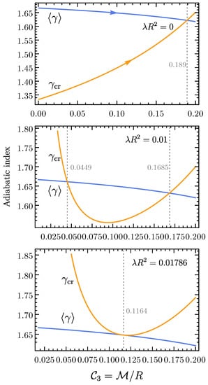
Figure 1. $N=3$: Pressure-averaged and critical adiabatic indices vs. compactness ${\mathcal{C}}_3$ given $\lambda \ge 0$. The configurations are unstable if $⟨\gamma ⟩<{\gamma }_{\mathrm{cr}}$, and the instabilities will set in at critical points $⟨\gamma ⟩={\gamma }_{\mathrm{cr}}$. In the case of zero cosmological constant $\lambda R^2=0$ (top), the arrows on the lines of adiabatic indices exhibit the directions when the fluid sphere is being compressed while keeping $\mathcal{M}$ fixed. There is only one critical point for the instability to be triggered at ${\mathcal{C}}_3=0.189$. On the other hand, if $\lambda >0$ is turned on (no matter how small it is), two critical points will present. It is shown that, for $\lambda R^2=0.01$ (middle), the stable region is bounded between ${\mathcal{C}}_3=0.0449$ and $0.1685$ and shrinks as $\lambda R^2$ increases until $\lambda R^2=0.01786$ (bottom), at which ${\mathcal{C}}_3=0.1164$, the two critical points, become degenerate. In Table 1, we list the corresponding compactness ${\mathcal{C}}_3$ and central velocity dispersion $v_c$ of stable regions with various $\lambda R^2\ge 0$.

Table 1. $N=3$: Stable regions $⟨\gamma ⟩\ge {\gamma }_{\mathrm{cr}}$ with various $\lambda R^2>0$. There is no stable configuration for $\lambda R^2\gtrsim 0.01786$.

$\mathit{\lambda }{\mathit{R}}^2$	${\mathcal{C}}_3=\mathcal{M}/\mathit{R}$	${\mathit{v}}_{\mathit{c}}=\mathit{v}\left(0\right)$	$⟨\mathit{\gamma }⟩$
0	$0–0.189057$	$0–0.681433$	$1.66667–1.62190$
$0.010$	$0.044912–0.16846$	$0.240284–0.604073$	$1.66116–1.63163$
$0.015$	$0.075802–0.149753$	$0.328969–0.541498$	$1.65634–1.63857$
$0.016$	$0.084228–0.14377$	$0.352167–0.522649$	$1.65483–1.64051$
$0.017$	$0.09501–0.13543$	$0.3818–0.497134$	$1.65275–1.64302$
$0.0175$	$0.10278–0.12889$	$0.403279–0.47766$	$1.65113–1.64485$
$0.0176$	$0.10485–0.12705$	$0.409033–0.472255$	$1.65069–1.64534$
$0.0177$	$0.10738–0.12475$	$0.416092–0.465544$	$1.65013–1.64594$
$0.0178$	$0.1109–0.1215$	$0.425964–0.456132$	$1.64933–1.64678$
$0.01785$	$0.1142–0.1183$	$0.435279–0.446946$	$1.64856–1.64757$
$0.01786$	$0.1164$	$0.441523$	$1.64804$

The stable configurations are bounded by the two critical points up to $\lambda R^2=0.01786$, above which there is no stable configuration, see Figure 1 (bottom). At this degenerate critical point, ${\mathcal{C}}_3=\mathcal{M}/R=0.1164$, we can eliminate the dependence of R to obtain $\mathcal{M}\sqrt{\lambda }=0.01556$, or $\mathcal{M}=0.01556\ell c^2/G_3$ with $G_3$ and c restored. Now, given the cosmological constant observed [56,57,58], $\ell \sim {10}^{61}{\ell }_{\mathrm{Pl}}$, where ${\ell }_{\mathrm{Pl}}$ is the Planck length in (3 + 1) dimensions, there is no stable stellar equilibrium for $\mathcal{M}\gtrsim 0.01556\ell c^2/G_3\sim {10}^{21}{\mathrm{M}}_{\odot }$. Therefore, a virialized mass sphere should be much smaller ${10}^{21}{\mathrm{M}}_{\odot }$ in order to have long-lived hydrostatic equilibrium before it can trigger the black hole formation. Curiously, this number is two orders of magnitude larger to the maximal Jeans mass (the threshold that a gas cloud can clump into gravitationally bound states) just prior to the recombination of hydrogen $M_{\mathrm{J}}\simeq 1.2\times {10}^{16}{\left({\mathsf{\Omega }}_{b,0}{h}^2\right)}^{-2}{\mathrm{M}}_{\odot }\simeq {10}^{19}{\mathrm{M}}_{\odot }$ with the current baryon abundance ${\mathsf{\Omega }}_{b,0}{h}^2\simeq 0.0224$ [57,59]. As the horizon mass of hydrogen is always less than the Jeans mass before recombination, structures can form only after recombination [60]. Therefore, the stable upper bound ${10}^{21}{\mathrm{M}}_{\odot }$ seems delicately protected in our universe.

On the other hand, a negative cosmological constant tends to stabilize the sphere due to the extra pressure and reduced energy density. Compared to zero and positive cosmological constant, the critical compactness becomes larger in order to trigger the collapse. There is only one critical point for a given compactness down to $\lambda R^2=-0.094853$, below which there is no physical solution due to causality ($v_c\le 1$). At this critical point, ${\mathcal{C}}_3=0.248$; see Figure 2.

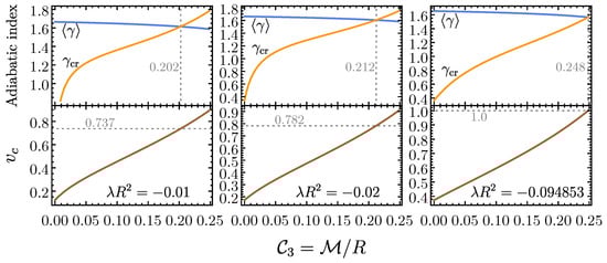
Figure 2. $N=3$: Pressure-averaged & critical adiabatic indices (top panels), and central velocity dispersion $v_c$ (bottom panels) vs. compactness ${\mathcal{C}}_3$ given $\lambda <0$. The configurations are unstable if $⟨\gamma ⟩<{\gamma }_{\mathrm{cr}}$, and the instabilities will set in at critical points $⟨\gamma ⟩={\gamma }_{\mathrm{cr}}$. There is only one critical point for $\lambda <0$. For $\lambda R^2=-0.01$ (left), the instability is to be triggered at ${\mathcal{C}}_3=0.202$ with $v_c=0.737$; however, for $\lambda R^2=-0.02$ (middle), it occurs at ${\mathcal{C}}_3=0.212$ with $v_c=0.782$. Compared to $\lambda R^2=0$ in Figure 1 (top), it becomes harder to trigger the instabilities as higher ${\mathcal{C}}_3$ (thus $v_c$) is required if $\lambda$ is more negative until $\lambda R^2=-0.094853$ (right), at which ${\mathcal{C}}_3=0.248$ with the causal limit $v_c=1$. Beyond this point, no physical configuration can trigger the instability on the grounds of causality. In Table 2, we list the critical points at causal limits for $N=3,4,5,6$ and 7.

For $N>3$, the fluid is genuinely unstable in NG. In GR, however, the fluid becomes stabilized if $\lambda <0$ is turned on. For $N=4,5,6$ and 7, we also identify the lower bound of $\lambda R^2$ in Table 2 that the fluid can still collapse into a black hole under the causal limit $v_c=1$.

Table 2. Critical points for $N=3,4,5,6,$ and 7 with $\lambda <0$ at causal limit $v_c=1$.

N	${\mathcal{C}}_{\mathit{N}}$	$\mathit{\lambda }{\mathit{R}}^2$	$⟨\mathit{\gamma }⟩={\mathit{\gamma }}_{\mathbf{cr}}$
3	$0.248179$	$-0.094853$	$1.56387$
4	$0.117505$	$-0.134605$	$1.43352$
5	$0.062846$	$-0.151149$	$1.35328$
6	$0.037099$	$-0.154395$	$1.29861$
7	$0.023595$	$-0.151406$	$1.25884$

4.2. Fluid Disks in (2 + 1)-Dimensional Spacetime

It is well known that (2 + 1) GR has no local degrees of freedom (locally flat), thus no gravitational wave (or graviton) can propagate. This means that particles do not gravitate if they are static in the (2 + 1)-dimensional spacetime [50,61,62]. On the other hand, the collective behavior of particles demands the fluid description under the influence of gravity [50]. To have hydrostatic equilibrium, a negative cosmological constant $\lambda =-1/{\ell }^2$ is to guarantee not only hydrostatic equilibrium [42] (the pressure is monotonically decreasing) but also permit a black hole solution (BTZ) in (2 + 1) dimensions. The metric interior to the fluid disk turns out to be

$$\mathrm{d}{s}_{\mathrm{disk}}^2=-e^{2\mathsf{\Phi }\left(r\right)}\mathrm{d}{t}^2+e^{2\mathsf{\Lambda }\left(r\right)}\mathrm{d}{r}^2+r^2\mathrm{d}{\varphi }^2\mathrm{with}{e}^{-2\mathsf{\Lambda }\left(r\right)}=1-2M\left(r\right)+\frac{r^2}{{\ell }^2}.$$

(38)

Note that, in (2 + 1) dimensions, the integration constant in $e^{-2\mathsf{\Lambda }\left(r\right)}$ is arbitrary, but it can always be normalized to “unity” by adjusting the natural mass scale $G_2$. On the other hand, the non-rotating BTZ metric reads

$$\mathrm{d}{s}_{\mathrm{BTZ}}^2=-f\left(r\right)\mathrm{d}{t}^2+\frac{\mathrm{d}{r}^2}{f\left(r\right)}+r^2\mathrm{d}{\varphi }^2\mathrm{with}f\left(r\right)=-{\mathcal{M}}_{\mathrm{BTZ}}+\frac{r^2}{{\ell }^2}.$$

(39)

To match spacetime of the fluid interior to the BTZ exterior, the junction condition at the fluid radius R leads to the relation of the BTZ mass and the fluid mass

$${\mathcal{M}}_{\mathrm{BTZ}}=2\mathcal{M}-1.$$

(40)

We note that the ADM mass in (2 + 1) is the BTZ mass [63,64,65], rather than the fluid mass. The phase diagrams of homogeneous fluid configurations with $0<\mathcal{M}\le 0.5$ and $\mathcal{M}>0.5$ are shown in Figure 3a,b, respectively. The absence of fluid $\mathcal{M}=0$ corresponds to the BTZ bound state (anti-de Sitter space) ${\mathcal{M}}_{\mathrm{BTZ}}=-1$, which is separated from the mass spectrum. The fluid mass $\mathcal{M}=0.5$ is the BTZ ground (vacuum) state ${\mathcal{M}}_{\mathrm{BTZ}}=0$. For $0<\mathcal{M}<0.5$, they are a sequence of states of naked conical singularity [63], $-1<{\mathcal{M}}_{\mathrm{BTZ}}<0$, if the fluid were to collapse. Furthermore, the threshold to have BTZ excited state ${\mathcal{M}}_{\mathrm{BTZ}}>0$ is $\mathcal{M}>0.5$. It is interesting to note that the central velocity dispersion $v_c$ is always monotonically increasing in $|\lambda R^2|$ for $0<\mathcal{M}\le 0.5$, while there are minima of $v_c\ne 0$ for $\mathcal{M}>0.5$, and no causal solution if $\mathcal{M}\gtrsim 0.5208$. This manifests that the two-phase diagrams are separated by the phase boundary$\mathcal{M}=0.5$ (or ${\mathcal{M}}_{\mathrm{BTZ}}=0$).

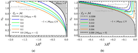
Figure 3. $v_c-\lambda R^2$ phase diagrams of homogeneous fluid disks in (2 + 1) dimensions with the total fluid mass (a) $0<\mathcal{M}\le 0.5 (-1<{\mathcal{M}}_{\mathrm{BTZ}}\le 0)$; (b) $\mathcal{M}>0.5 ({\mathcal{M}}_{\mathrm{BTZ}}>0)$. The BTZ bound state (AdS spacetime) ${\mathcal{M}}_{\mathrm{BTZ}}=-1$ ($\mathcal{M}=0$ only if $R=0$ as $\rho \ne 0$) is separated from the mass spectrum. The fluid solution for $\mathcal{M}\gtrsim 0.5208$ is forbidden regarding causality. In Appendix F, we list the corresponding $\lambda R^2$ at causal limit $v_c=1$ for various $0<\mathcal{M}\le 0.5$ in Table A1 and $\mathcal{M}>0.5$ in Table A2, respectively. The minima of $v_c$ for $\mathcal{M}>0.5$ are shown in Table A3.

By Chandrasekhar’s criterion at the critical point $⟨\gamma ⟩={\gamma }_{\mathrm{cr}}$, we can examine if the BTZ excited states and the BTZ bound states (naked singularities) can result from a collapsing fluid. For a homogeneous disk, the critical adiabatic index, Equation (37), reduces to

$$\begin{array}{cc}\hfill {\gamma }_{\mathrm{cr}}=-1& +\sum _{j,k=0,1,\dots }{f}_{jk}^{\left(2\right)}{\mathcal{M}}^j{\left(\lambda R^2\right)}^k=\left(-\frac{1}{3}\left(\lambda R^2\right)-\frac{11}{72}{\left(\lambda R^2\right)}^2-\frac{37}{432}{\left(\lambda R^2\right)}^3+\dots \right)\hfill \\ \hfill & +\left(-\frac{3}{4}\left(\lambda R^2\right)-\frac{3}{4}{\left(\lambda R^2\right)}^2-\frac{125}{192}{\left(\lambda R^2\right)}^3+\dots \right)\mathcal{M}\hfill \\ \hfill & +\left(-\frac{19}{12}\left(\lambda R^2\right)-\frac{733}{288}{\left(\lambda R^2\right)}^2-\frac{439}{144}{\left(\lambda R^2\right)}^3+\dots \right){\mathcal{M}}^2\hfill \\ \hfill & +\left(-\frac{157}{48}\left(\lambda R^2\right)-\frac{133}{18}{\left(\lambda R^2\right)}^2-\frac{821}{72}{\left(\lambda R^2\right)}^3+\dots \right){\mathcal{M}}^3+\mathcal{O}\left({\mathcal{M}}^4\right).\hfill \end{array}$$

(41)

It ostensibly starts from “zero” rather than “one” in NG as $\lambda R^2\to 0$. However, Equation (41) is not necessarily convergent to zero as $\lambda R^2\to 0$, and the convergence really relies on the fluid mass $\mathcal{M}$. In fact, ${\gamma }_{\mathrm{cr}}\to 0$ as $\lambda R^2\to 0$only if$\mathcal{M}\le 0.5$ when the fluid is being compressed. Thus, the presence of the negative cosmological constant makes the relativistic instability hardly be triggered for $\mathcal{M}\le 0.5$. In Figure 4 (left), we take $\mathcal{M}=0.4$, for example, and it is always ${\gamma }_{\mathrm{cr}}<⟨\gamma ⟩$, thus stable, under causal region $v_c\le 1$. On the other hand, the instability could set in if the fluid disk exceeds, no matter how tiny amount, the threshold $\mathcal{M}=0.5$ (or ${\mathcal{M}}_{\mathrm{BTZ}}=0$). Nevertheless, some external agent must compress the fluid to make it unstable if $\lambda$ is fixed. In Figure 4 (middle), for $\mathcal{M}=0.508$, the instability can set in at $\lambda R^2=-0.0247$ with central velocity dispersion $v_c=0.799$. For higher $\mathcal{M}$, both $|\lambda R^2|$ and $v_c$ increase at the critical point of instability until $\mathcal{M}=0.518$ at $\lambda R^2=-0.0609$ with $v_c=1$. Beyond this mass, there is no unstable configuration under causal range $v_c\le 1$. In Appendix F, we also list the critical points ($\lambda R^2,v_c$) of instability for various masses $0.5<\mathcal{M}\lesssim 0.518$ in Table A4.

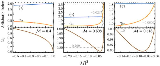
Figure 4. $N=2$: Pressure-averaged and critical adiabatic indices (top panels), and central velocity dispersion $v_c$ (bottom panels) vs. curvature parameter $\lambda R^2$. The configurations are unstable if $⟨\gamma ⟩<{\gamma }_{\mathrm{cr}}$, and the instabilities will set in at critical points $⟨\gamma ⟩={\gamma }_{\mathrm{cr}}$. The arrows on the lines of adiabatic indices exhibit the directions when the fluid sphere is being compressed while keeping ${\mathcal{C}}_2=\mathcal{M}$ and $\lambda$ fixed. For $\mathcal{M}\le 0.5$, there is no crossing of the two indices, thus no instability will be triggered. For example, for $\mathcal{M}=0.4$ (left), ${\gamma }_{\mathrm{cr}}$ ($⟨\gamma ⟩$) is maximal (minimal) at $v_c=1$ and decreases down (increases up) to zero (two) as R decreases and the two indices never cross. On the contrary, instabilities can occur for $\mathcal{M}>0.5$. For $\mathcal{M}=0.508$ (middle), the instability can set in at $\lambda R^2=-0.0247$ with $v_c=0.799$; however, for $\mathcal{M}=0.518$ (right), it is at $\lambda R^2=-0.0609$ with $v_c=1$; no instability can be triggered if $\mathcal{M}\gtrsim 0.518$ regarding causality.

5. Discussions and Implications

We have derived Chandrasekhar’s criterion in (N + 1) spacetime with and without cosmological constant. As an illustration, we take the homogeneous solution to determine the instability provided that the sphere is composed of an ideal monatomic fluid.

In (3 + 1) spacetime, the privileged position is manifest as it is the marginal dimensionality in which the fluid sphere is stable but not too stable to trigger the onset of gravitational collapse. In particular, it is the unique dimensionality that allows a stable hydrostatic equilibrium with a positive cosmological constant. For higher spatial dimensions, the fluid sphere is genuinely unstable either in the context of NG or GR. However, a negative cosmological constant can stabilize it.

In (2 + 1) spacetime, the effect of negative cosmological constant wins the relativistic effect so that it is too stable for a fluid disk of mass $0<\mathcal{M}\le 0.5$ to collapse into a naked singularity. This somewhat supports the Cosmic Censorship Conjecture [66]. However, the BTZ hole emergence is possible from a collapsing fluid under proper conditions. This is reasonable because, if it were not the case, the anti-de Sitter space ${\mathcal{M}}_{\mathrm{BTZ}}=-1$ (bound state) could be deformed continuously into a BTZ black hole of mass ${\mathcal{M}}_{\mathrm{BTZ}}\ge 0$ (vacuum or excited state) by growing the mass of the fluid disk from $\mathcal{M}=0$ to $\mathcal{M}\ge 0.5$.

We now summarize the assumptions made implicitly in the results and the implications:

Assumptions:

• First law of thermodynamics and equipartition theorem hold;
• Mass–energy dispersion relation $E=\sqrt{{\mathbf{p}}^2+m^2}$ is valid;
• Einstein equations hold in (N + 1) dimensions.

The particles in a fluid sphere (or disk) are well thermalized at each local point in the spacetime such that the equipartition theorem holds; thus, the pressure is isotropic macroscopically. Microscopically, every particle in the fluid follows the mass–energy relation if the Lorentz symmetry is locally preserved. This is based on the assumption that particle states can be described by vectors in some irreducible representation of the Poincaré group; however, Lorentz symmetry is not necessary if the vectors describing particles can be generated from a vacuum vector with the help of local field operators [67]. In the fluid description, its adiabatic index can vary from $1+2/N$ to $1+1/N$ as particles go from non-relativistic to ultra-relativistic regimes as more and more gravitational energy is converted into the fluid. On the gravity side, we restrict to only “one time dimension” since the hyperbolicity of field equations (in this note GR or its Newtonian limit) determines the causal structure [8], hence the “predictivity” allows physicists to do theoretical physics. Moreover, in view of the Ostrogradsky theorem [68], the field equations are at most second derivative because equations of motion with higher-order derivatives are in principle unstable or non-local. Both GR and NG are free of Ostrogradsky instability.

Although the gravitational attraction of a fluid is becoming weaker as space dimension N increases, its pressure is even weaker when being compressed because the randomly moving particles inside the fluid will have more directions to go, and thus be easier to collapse. This is the reason why an ideal monatomic fluid is genuinely unstable in higher dimensions:

Implications:

• Baby universe emerges from collapsing matter in a black hole;
• Spacetime dimensionality reshuffles in the reign of quantum gravity.

We can reexamine the idea that the observable universe is the interior of a black hole [69,70,71,72,73,74] existing as one of possibly many inside a larger parent universe, or multiverse. Since singularity is generic [75,76,77,78,79] in GR, some limiting curvature must exist [80,81] to avoid the singularity formation and transition to a baby universe. Several mechanisms, including extended GR with torsion [82], invoking stringy Hagedorn matter [24,83] to produce a bouncing solution [84,85], braneworld scenario [86,87], or transition through an S-brane [88], have been introduced to realize the idea.

Suppose the space dimension reshuffling is a random process as collapsing matter into a black hole in a universe of arbitrary space dimension N. When the collapsing matter is squeezed down to the Planck scale (near the classical black hole singularity), it would emerge to a new universe with different space dimensions. The change of spacetime dimensions through phase transition near the Planck scale might require some unknown theory of quantum gravity or string theory [11,12]. Some inflation models that predict parts of exponentially large size having different dimensionalities [89] might provide an alternative mechanism. This process will repeat again and again until the new-born universe is just (3 + 1)-dimensional, which is stable but not too stable for the pristine gas in it to form complicated structures, including both black holes and stars. In any higher dimensions $N>3$, it is too easy for matter to collapse into black holes; and in (2 + 1), there is no way to form black holes from self-gravitating fluid without external agents—Both are too barren to have complex structures.

The above discussion reverberates the anthropic principle [5,6,90,91,92] in one way or another, though it only relies on the assumptions regardless of the anthropic reasoning. However, it tells more than that because gravitationally bound states of monatomic fluid are genuinely unstable and bound to black holes immediately in space dimensions higher than three. Although a negative cosmological constant could stabilize the fluid spheres, it decelerates the expansion of the whole universe on a large scale. This leads to another issue on the anthropic bound of cosmological constant [6,92,93], even though the falsifiability has been criticized [94,95]. In (3 + 1), the anthropic bound on the positive cosmological constant [96] argues that it could not be very large, or the universe would expand too fast for galaxies or stars (or us) to form. While once these local structures are detached from the background expansion, its smallness also prevents the gravitationally bound state (typically of mass much less than ${10}^{21}{\mathrm{M}}_{\odot }$) from forming a black hole immediately given the current cosmological constant observed.

Why $N=3$? Perhaps the more sensible question is not what makes (3 + 1) the preferred dimensionality [9,10,11,12], but, rather, why the physical principles (thermodynamics, Lorentz symmetry, GR,…) allow fecund universes to exist only in (3 + 1), which is the unique dimensionality that permits stable hydrostatic equilibrium with a positive cosmological constant.

References

- Ehrenfest, P. In what way does it become manifest in the fundamental laws of physics that space has three dimensions? Proc. Amst. Acad. 1918, 20, 200–209. [Google Scholar]
- Ehrenfest, P. Welche Rolle spielt die Dreidimensionalität des Raumes in den Grundgesetzen der Physik? Ann. Phys. 1920, 366, 440–446. [Google Scholar] [CrossRef]
- Whitrow, G.J. Why Physical Space Has Three Dimensions. Br. J. Philos. Sci. 1955, 6, 13–31. [Google Scholar] [CrossRef]
- Tangherlini, F.R. Schwarzschild field in n dimensions and the dimensionality of space problem. Nuovo Cim. 1963, 27, 636–651. [Google Scholar] [CrossRef]
- Barrow, J.D. Dimensionality. Philos. Trans. R. Soc. Lond. A 1983, 310, 337–346. [Google Scholar] [CrossRef]
- Barrow, J.D.; Tipler, F.J. The Anthropic Cosmological Principle; Oxford University Press: Oxford, UK, 1988. [Google Scholar]
- Caruso, F.; Moreira Xavier, R. On the Physical Problem of Spatial Dimensions: An Alternative Procedure to Stability Arguments. Fund. Sci. 1987, 8, 73–91. [Google Scholar]
- Tegmark, M. On the dimensionality of space-time. Class. Quant. Grav. 1997, 14, L69–L75. [Google Scholar] [CrossRef]
- Momen, A.; Rahman, R. Spacetime Dimensionality from de Sitter Entropy. TSPU Bull. 2014, 12, 186–191. [Google Scholar]
- Gonzalez-Ayala, J.; Cordero, R.; Angulo-Brown, F. Is the (3 + 1)-d nature of the universe a thermodynamic necessity? EPL 2016, 113, 40006. [Google Scholar] [CrossRef]
- Brandenberger, R.H.; Vafa, C. Superstrings in the Early Universe. Nucl. Phys. B 1989, 316, 391–410. [Google Scholar] [CrossRef]
- Greene, B.; Kabat, D.; Marnerides, S. On three dimensions as the preferred dimensionality of space via the Brandenberger-Vafa mechanism. Phys. Rev. D 2013, 88, 043527. [Google Scholar] [CrossRef]
- Durrer, R.; Kunz, M.; Sakellariadou, M. Why do we live in 3 + 1 dimensions? Phys. Lett. B 2005, 614, 125–130. [Google Scholar] [CrossRef]
- Nielsen, H.B.; Rugh, S.E. Why do we live in (3 + 1)-dimensions? In Proceedings of the 26th International Ahrenshoop Symposium on the Theory of Elementary Particles, Buckow, Germany, 27–31 August 1993. [Google Scholar]
- Deser, S. Why does D=4, rather than more (or less)? An Orwellian explanation. Proc. R. Soc. Lond. A 2020, 476, 20190632. [Google Scholar] [CrossRef]
- Carlip, S. Dimension and Dimensional Reduction in Quantum Gravity. Class. Quant. Grav. 2017, 34, 193001. [Google Scholar] [CrossRef]
- Pardo, K.; Fishbach, M.; Holz, D.E.; Spergel, D.N. Limits on the number of spacetime dimensions from GW170817. JCAP 2018, 7, 48. [Google Scholar] [CrossRef]
- Scargill, J.H.C. Can Life Exist in 2 + 1 Dimensions? Phys. Rev. Res. 2020, 2, 013217. [Google Scholar] [CrossRef]
- Ponce de Leon, J.; Cruz, N. Hydrostatic equilibrium of a perfect fluid sphere with exterior higher dimensional Schwarzschild space-time. Gen. Rel. Grav. 2000, 32, 1207–1216. [Google Scholar] [CrossRef]
- Paul, B.C. Relativistic star solutions in higher dimensions. Int. J. Mod. Phys. D 2004, 13, 229–238. [Google Scholar] [CrossRef]
- Zarro, C.A.D. Buchdahl limit for d-dimensional spherical solutions with a cosmological constant. Gen. Rel. Grav. 2009, 41, 453–468. [Google Scholar] [CrossRef]
- Buchdahl, H.A. General Relativistic Fluid Spheres. Phys. Rev. 1959, 116, 1027. [Google Scholar] [CrossRef]
- Goswami, R.; Maharaj, S.D.; Nzioki, A.M. Buchdahl-Bondi limit in modified gravity: Packing extra effective mass in relativistic compact stars. Phys. Rev. D 2015, 92, 064002. [Google Scholar] [CrossRef]
- Feng, W.X.; Geng, C.Q.; Luo, L.W. The Buchdahl stability bound in Eddington-inspired Born-Infeld gravity. Chin. Phys. C 2019, 43, 083107. [Google Scholar] [CrossRef]
- Chakraborty, S.; Dadhich, N. Universality of the Buchdahl sphere. arXiv 2022, arXiv:2204.10734. [Google Scholar]
- Chandrasekhar, S. Dynamical Instability of Gaseous Masses Approaching the Schwarzschild Limit in General Relativity. Phys. Rev. Lett. 1964, 12, 114–116. [Google Scholar] [CrossRef]
- Chandrasekhar, S. The Dynamical Instability of Gaseous Masses Approaching the Schwarzschild Limit in General Relativity. Astrophys. J. 1964, 140, 417–433, Erratum in: Astrophys. J. 1964, 140, 1342. [Google Scholar] [CrossRef]
- Zel’dovich, Y.B.; Podurets, M.A. The Evolution of a System of Gravitationally Interacting Point Masses. Sov. Astron. 1966, 9, 742. [Google Scholar]
- Ipser, J.R. A binding-energy criterion for the dynamical stability of spherical stellar systems in general relativity. Astrophys. J. 1980, 238, 1101. [Google Scholar] [CrossRef]
- Günther, S.; Straub, C.; Rein, G. Collisionless equilibria in general relativity: Stable configurations beyond the first binding energy maximum. Astrophys. J. 2021, 918, 48. [Google Scholar] [CrossRef]
- Feng, W.X.; Yu, H.B.; Zhong, Y.M. Dynamical Instability of Collapsed Dark Matter Halos. JCAP 2022, 5, 36. [Google Scholar] [CrossRef]
- Lynden-Bell, D.; Wood, R. The gravo-thermal catastrophe in isothermal spheres and the onset of red-giant structure for stellar systems. Mon. Not. R. Astron. Soc. 1968, 138, 495. [Google Scholar] [CrossRef]
- Spitzer, L. Dynamical Evolution of Globular Clusters; Princeton University Press: Princeton, NJ, USA, 1987. [Google Scholar]
- Boehmer, C.G.; Harko, T. Dynamical instability of fluid spheres in the presence of a cosmological constant. Phys. Rev. D 2005, 71, 084026. [Google Scholar] [CrossRef]
- Posada, C.; Hladík, J.; Stuchlík, Z. Dynamical instability of polytropic spheres in spacetimes with a cosmological constant. Phys. Rev. D 2020, 102, 024056. [Google Scholar] [CrossRef]
- Arbañil, J.D.V.; Carvalho, G.A.; Lobato, R.V.; Marinho, R.M.; Malheiro, M. Extra dimensions’ influence on the equilibrium and radial stability of strange quark stars. Phys. Rev. D 2019, 100, 024035. [Google Scholar] [CrossRef]
- Haemmerlé, L. General-relativistic instability in hylotropic supermassive stars. Astron. Astrophys. 2020, 644, A154. [Google Scholar] [CrossRef]
- Feng, W.X.; Yu, H.B.; Zhong, Y.M. Seeding Supermassive Black Holes with Self-Interacting Dark Matter: A Unified Scenario with Baryons. Astrophys. J. Lett. 2021, 914, L26. [Google Scholar] [CrossRef]
- Roupas, Z. Relativistic Gravothermal Instabilities. Class. Quant. Grav. 2015, 32, 135023. [Google Scholar] [CrossRef]
- Roupas, Z.; Chavanis, P.H. Relativistic Gravitational Phase Transitions and Instabilities of the Fermi Gas. Class. Quant. Grav. 2019, 36, 065001. [Google Scholar] [CrossRef]
- Roupas, Z. Relativistic Gravitational Collapse by Thermal Mass. Commun. Theor. Phys. 2021, 73, 015401. [Google Scholar] [CrossRef]
- Cruz, N.; Zanelli, J. Stellar equilibrium in (2 + 1)-dimensions. Class. Quant. Grav. 1995, 12, 975–982. [Google Scholar] [CrossRef]
- Banados, M.; Teitelboim, C.; Zanelli, J. The Black hole in three-dimensional space-time. Phys. Rev. Lett. 1992, 69, 1849–1851. [Google Scholar] [CrossRef]
- Ross, S.F.; Mann, R.B. Gravitationally collapsing dust in (2 + 1)-dimensions. Phys. Rev. D 1993, 47, 3319–3322. [Google Scholar] [CrossRef]
- Pretorius, F.; Choptuik, M.W. Gravitational collapse in (2 + 1)-dimensional AdS space-time. Phys. Rev. D 2000, 62, 124012. [Google Scholar] [CrossRef]
- Husain, V.; Olivier, M. Scalar field collapse in three-dimensional AdS space-time. Class. Quant. Grav. 2001, 18, L1–L10. [Google Scholar] [CrossRef]
- Jałmużna, J.; Gundlach, C.; Chmaj, T. Scalar field critical collapse in 2 + 1 dimensions. Phys. Rev. D 2015, 92, 124044. [Google Scholar] [CrossRef]
- Bourg, P.; Gundlach, C. Critical collapse of a spherically symmetric ultrarelativistic fluid in 2 + 1 dimensions. Phys. Rev. D 2021, 103, 124055. [Google Scholar] [CrossRef]
- Bourg, P.; Gundlach, C. Critical collapse of an axisymmetric ultrarelativistic fluid in 2 + 1 dimensions. Phys. Rev. D 2021, 104, 104017. [Google Scholar] [CrossRef]
- Giddings, S.; Abbott, J.; Kuchar, K. Einstein’s theory in a three-dimensional space-time. Gen. Rel. Grav. 1984, 16, 751–775. [Google Scholar] [CrossRef]
- Ogilvie, G.I. Astrophysical fluid dynamics. J. Plasma Phys. 2016, 82, 205820301. [Google Scholar] [CrossRef]
- Tooper, R.F. Adiabatic Fluid Spheres in General Relativity. Astrophys. J. 1965, 142, 1541. [Google Scholar] [CrossRef]
- Shapiro, S.L.; Teukolsky, S.A. Black Holes, White Dwarfs, and Neutron Stars: The Physics of Compact Objects; John Wiley and Sons: Hoboken, NJ, USA, 1983. [Google Scholar]
- Axenides, M.; Georgiou, G.; Roupas, Z. Gravothermal Catastrophe with a Cosmological Constant. Phys. Rev. D 2012, 86, 104005. [Google Scholar] [CrossRef]
- Feng, W.X. Gravothermal phase transition, black holes and space dimensionality. Phys. Rev. D 2022, 106, L041501. [Google Scholar] [CrossRef]
- Ade, P.A.R.; Aghanim, N.; Arnaud, M.; Ashdown, M.; Aumont, J.; Baccigalupi, C.; Banday, A.J.; Barreiro, R.B.; Bartlett, J.G.; Bartolo, N.; et al. Planck 2015 results. XIII. Cosmological parameters. Astron. Astrophys. 2016, 594, A13. [Google Scholar] [CrossRef]
- Aghanim, N.; Akrami, Y.; Ashdown, M.; Aumont, J.; Baccigalupi, C.; Ballardini, M.; Banday, A.J.; Barreiro, R.B.; Bartolo, N.; Basak, S.; et al. Planck 2018 results. VI. Cosmological parameters. Astron. Astrophys. 2020, 641, A6, Erratum: Astron. Astrophys. 2021, 652, C4. [Google Scholar] [CrossRef]
- Prat, J.; Hogan, C.; Chang, C.; Frieman, J. Vacuum energy density measured from cosmological data. JCAP 2022, 6, 15. [Google Scholar] [CrossRef]
- Mo, H.; van den Bosch, F.; White, S. Galaxy Formation and Evolution; Cambridge University Press: Cambridge, MA, USA, 2010. [Google Scholar]
- Kolb, E.W.; Turner, M.S. The Early Universe; Addison-Wesley Publishing: Boston, MA, USA, 1990; Volume 69. [Google Scholar]
- Deser, S.; Jackiw, R.; ’t Hooft, G. Three-Dimensional Einstein Gravity: Dynamics of Flat Space. Ann. Phys. 1984, 152, 220. [Google Scholar] [CrossRef]
- Deser, S.; Jackiw, R. Three-Dimensional Cosmological Gravity: Dynamics of Constant Curvature. Ann. Phys. 1984, 153, 405–416. [Google Scholar] [CrossRef]
- Banados, M.; Henneaux, M.; Teitelboim, C.; Zanelli, J. Geometry of the (2 + 1) black hole. Phys. Rev. D 1993, 48, 1506–1525, Erratum: Phys. Rev. D 2013, 88, 069902. [Google Scholar] [CrossRef]
- Brown, J.D.; Henneaux, M. Central Charges in the Canonical Realization of Asymptotic Symmetries: An Example from Three-Dimensional Gravity. Commun. Math. Phys. 1986, 104, 207–226. [Google Scholar] [CrossRef]
- Brown, J.D.; Creighton, J.; Mann, R.B. Temperature, energy and heat capacity of asymptotically anti-de Sitter black holes. Phys. Rev. D 1994, 50, 6394–6403. [Google Scholar] [CrossRef]
- Penrose, R. Gravitational collapse: The role of general relativity. Riv. Nuovo Cim. 1969, 1, 252–276. [Google Scholar] [CrossRef]
- Borchers, H.J.; Buchholz, D. The Energy Momentum Spectrum in Local Field Theories With Broken Lorentz Symmetry. Commun. Math. Phys. 1985, 97, 169. [Google Scholar] [CrossRef]
- Woodard, R.P. Ostrogradsky’s theorem on Hamiltonian instability. Scholarpedia 2015, 10, 32243. [Google Scholar] [CrossRef]
- Pathria, R.K. The Universe as a Black Hole. Nature 1972, 240, 298–299. [Google Scholar] [CrossRef]
- Good, I.J. Chinese universes. Phys. Today 1972, 25, 15. [Google Scholar] [CrossRef]
- Easson, D.A.; Brandenberger, R.H. Universe generation from black hole interiors. JHEP 2001, 6, 24. [Google Scholar] [CrossRef]
- Gaztanaga, E.; Fosalba, P. A Peek Outside Our Universe. Symmetry 2022, 14, 285. [Google Scholar] [CrossRef]
- Gaztanaga, E. How the Big Bang Ends Up Inside a Black Hole. Universe 2022, 8, 257. [Google Scholar] [CrossRef]
- Roupas, Z. Detectable universes inside regular black holes. Eur. Phys. J. C 2022, 82, 255. [Google Scholar] [CrossRef]
- Penrose, R. Gravitational collapse and space-time singularities. Phys. Rev. Lett. 1965, 14, 57–59. [Google Scholar] [CrossRef]
- Hawking, S. Occurrence of singularities in open universes. Phys. Rev. Lett. 1965, 15, 689–690. [Google Scholar] [CrossRef]
- Geroch, R.P. Singularities in closed universes. Phys. Rev. Lett. 1966, 17, 445–447. [Google Scholar] [CrossRef]
- Ellis, G.F.R.; Hawking, S. The Cosmic black body radiation and the existence of singularities in our universe. Astrophys. J. 1968, 152, 25. [Google Scholar] [CrossRef]
- Garfinkle, D. Numerical simulations of generic singularities. Phys. Rev. Lett. 2004, 93, 161101. [Google Scholar] [CrossRef]
- Frolov, V.P.; Markov, M.A.; Mukhanov, V.F. Black Holes as Possible Sources of Closed and Semiclosed Worlds. Phys. Rev. D 1990, 41, 383. [Google Scholar] [CrossRef]
- Frolov, V.P.; Markov, M.A.; Mukhanov, V.F. Through a black hole into a New Universe? Phys. Lett. B 1989, 216, 272–276. [Google Scholar] [CrossRef]
- Popławski, N.J. Cosmology with torsion: An alternative to cosmic inflation. Phys. Lett. B 2010, 694, 181–185, Erratum in Phys. Lett. B 2011, 701, 672–672. [Google Scholar] [CrossRef]
- Dubovsky, S.; Flauger, R.; Gorbenko, V. Solving the Simplest Theory of Quantum Gravity. JHEP 2012, 9, 133. [Google Scholar] [CrossRef]
- Biswas, T.; Mazumdar, A.; Siegel, W. Bouncing universes in string-inspired gravity. JCAP 2006, 3, 9. [Google Scholar] [CrossRef]
- Biswas, T.; Brandenberger, R.; Mazumdar, A.; Siegel, W. Non-perturbative Gravity, Hagedorn Bounce & CMB. JCAP 2007, 12, 11. [Google Scholar] [CrossRef]
- Dvali, G.R.; Gabadadze, G.; Porrati, M. 4-D gravity on a brane in 5-D Minkowski space. Phys. Lett. B 2000, 485, 208–214. [Google Scholar] [CrossRef]
- Pourhasan, R.; Afshordi, N.; Mann, R.B. Out of the White Hole: A Holographic Origin for the Big Bang. JCAP 2014, 4, 5. [Google Scholar] [CrossRef]
- Brandenberger, R.; Heisenberg, L.; Robnik, J. Non-singular black holes with a zero-shear S-brane. JHEP 2021, 5, 90. [Google Scholar] [CrossRef]
- Linde, A.D.; Zelnikov, M.I. Inflationary Universe With Fluctuating Dimension. Phys. Lett. B 1988, 215, 59–63. [Google Scholar] [CrossRef]
- Smolin, L. The Life of the Cosmos; Oxford University Press: Oxford, UK, 1999. [Google Scholar]
- Susskind, L. The Anthropic landscape of string theory. arXiv 2003, arXiv:hep-th/0302219. [Google Scholar]
- Linde, A.D. Inflation, quantum cosmology and the anthropic principle. arXiv 2002, arXiv:hep-th/0211048. [Google Scholar]
- Bousso, R.; Polchinski, J. The string theory landscape. Sci. Am. 2004, 291, 78–87. [Google Scholar] [CrossRef]
- Ball, P. Mysterious cosmos. Nature 2004. [Google Scholar] [CrossRef]
- Smolin, L. Scientific alternatives to the anthropic principle. arXiv 2004, arXiv:hep-th/0407213. [Google Scholar]
- Weinberg, S. Anthropic Bound on the Cosmological Constant. Phys. Rev. Lett. 1987, 59, 2607. [Google Scholar] [CrossRef]
Disclaimer/Publisher’s Note: The statements, opinions and data contained in all publications are solely those of the individual author(s) and contributor(s) and not of MDPI and/or the editor(s). MDPI and/or the editor(s) disclaim responsibility for any injury to people or property resulting from any ideas, methods, instructions or products referred to in the content. |
© 2023 by the author. Licensee MDPI, Basel, Switzerland. This article is an open access article distributed under the terms and conditions of the Creative Commons Attribution (CC BY) license (https://creativecommons.org/licenses/by/4.0/).