
Mid-to-Long Range Wind Forecast in Brazil Using Numerical Modeling and Neural Networks
by
 ,
,
Ricardo M. Campos
1 ,
,
Ronaldo M. J. Palmeira
2,3, 
Henrique P. P. Pereira
2,4 and
Laura C. Azevedo
2,5,* 1
Cooperative Institute for Marine and Atmospheric Studies (CIMAS), NOAA/Atlantic Oceanographic and Meteorological Laboratory (AOML), 4301 Rickenbacker Causeway, Miami, FL 33149, USA
2
AtmosMarine, Ilha do Fundão, Rua Hélio de Almeida, Cidade Universitária, Rio de Janeiro 21941-614, RJ, Brazil
3
Departamento de Ciências Atmosféricas, Instituto de Astronomia, Geofísica e Ciências Atmosféricas (IAG-USP), Universidade de São Paulo (USP), R. do Matão, 1226-Butantã, São Paulo 05508-090, SP, Brazil
4
Programa de Engenharia Oceânica COPPE, Universidade Federal do Rio de Janeiro, Cidade Universitária, Ilha do Fundão, Rio de Janeiro 21945-970, RJ, Brazil
5
Center for Maritime and Port Studies, University South Florida, 140 7th Avenue South, St. Petersburg, FL 33701, USA
*
Author to whom correspondence should be addressed.
Wind 2022, 2(2), 221-245; https://doi.org/10.3390/wind2020013
Submission received: 22 February 2022
/
Revised: 14 April 2022
/
Accepted: 19 April 2022
/
Published: 22 April 2022
Abstract
:This paper investigated the development of a hybrid model for wind speed forecast, ranging from 1 to 46 days, in the northeast of Brazil. The prediction system was linked to the widely used numerical weather prediction from the ECMWF global ensemble forecast, with neural networks (NNs) trained using local measurements. The focus of this study was on the post-processing of NNs, in terms of data structure, dimensionality, architecture, training strategy, and validation. Multilayer perceptron NNs were constructed using the following inputs: wind components, temperature, humidity, and atmospheric pressure information from ECMWF, as well as latitude, longitude, sin/cos of time, and forecast lead time. The main NN output consisted of the residue of wind speed, i.e., the difference between the arithmetic ensemble mean, derived from ECMWF, and the observations. By preserving the simplicity and small dimension of the NN model, it was possible to build an ensemble of NNs (20 members) that significantly improved the forecasts. The original ECMWF bias of −0.3 to −1.4 m/s has been corrected to values between −0.1 and 0.1 m/s, while also reducing the RMSE in 10 to 30%. The operational implementation is discussed, and a detailed evaluation shows the considerable generalization capability and robustness of the forecast system, with low computational cost.
1. Introduction
Wind forecasts play an important role in environmental prediction, where surface winds directly respond to atmospheric disturbances while also driving a variety of ocean effects, including gravity waves, surface currents, and sea level changes. In the renewable energy sector, the accuracy of such forecasts impacts the estimated energy production, leading to a series of economic and social consequences both in the short and long terms. According to the Global Wind Energy Council [1] and the International Renewable Energy Agency 2021 [2], Brazil holds the eighth position in the global ranking of wind energy, with 17 GW of installed capacity, coming from more than 750 wind farms and 10.000 wind turbines. Most of them (89%) are located in the northeast of Brazil, at tropical latitudes between 15° S to 0° N. Moreover, as reported by Associação Brasileira de Energia Eólica (ABEEólica, [3]), Brazil has a wind power potential to reach 500 GW, which would attend three times the current country’s energy demand.
Vinhoza and Schaeffer [4] assessed the wind energy potential in Brazil using a spatial approach, mapping the most economically attractive areas for offshore wind deployment. Santos et al. [5] and Silva et al. [6] investigated the wind energy utilization in Brazil in terms of its regulatory framework and national opportunities, describing the existence of a vast and reliable wind potential for immediate utilization in Brazil. Interestingly, Filgueiras and Silva [7] and Lima and Mendes [8] discuss that the overall power generation in Brazil is predominantly hydroelectric, which has led to an increasing vulnerability under changes in the global and local climate [9], with impacts on the hydrological cycle; however, considering the seasonal cycle, the country reaches the highest wind speed exactly when the rate flow of the main rivers is low—raising the strategic importance of wind energy expansion, combined with high-quality environmental predictions. Therefore, wind forecasts in the northeast of Brazil have gathered a wide range of applications and demands.
Several high-quality wind forecast systems have been developed in recent years, using either numerical weather prediction models (NWP) or machine learning models. Jacondino et al. [10] produced an hourly day-ahead wind speed forecast for two wind farms in northeast Brazil using the NWP model WRF (Weather Research and Forecasting; [11]), where sensitivity experiments with different physical options were evaluated. Zucatelli et al. [12] developed a recurrent neural network to perform 1 h wind forecasts in Brazil, following a recursive application for the subsequent hours. Samet et al. [13] provided an evaluation of neural network-based methodologies for wind speed forecasting using multi-layer perceptron neural networks. Additional examples of artificial intelligence for wind forecasts worldwide are referred [14,15,16,17,18,19,20,21,22,23,24]. However, all the aforementioned studies are focused on short-term forecasts, covering time scales of hours to a few days, whereas the mid-to-long term forecasts beyond 10 days remain uncovered and with a large demand. Even the recent study [25], for example, which aimed at relative long-term predictions according to authors, was bounded to a 3 day forecast.
In this context, the present study proposes a new wind forecast system focused on forecast ranges from 1 to 46 days, with special attention to the subseasonal scale. Our goal was to combine the traditional NWP global models, where the coarse resolution does not capture regional features, with multilayer perceptron neural networks (MLP-NN, [26]) trained with local measurements. Such a hybrid approach has been used by Xu et al. [27], who argued that the current mainstream method for wind speed forecasting involves the combination of numerical meteorological models with statistical post-processing; nevertheless, their system is also restricted to 72 h forecasts, while our present study evolves this period to 46 days.
This initiative has been conceived for operational applications, i.e., the forecast system must be reliable, simple to maintain and to fix, with low computational cost, and robust. This paper starts with a description of the local wind characteristics in the northeast of Brazil (Section 2.1), then it explains the numerical weather prediction using a global ensemble forecast and its importance for mid-to-long forecast ranges (Section 2.2), followed by its evaluation in Section 3. Section 4 describes the neural network model for post-processing. The results of the hybrid model, combining the NWP model and the NN model, are presented in Section 5 and discussed in Section 6, including the operational application of the new prediction system. The conclusions and future plans are described in Section 7. The research steps followed throughout this paper are summarized in the next Figure 1.
Finally, it is import to highlight that wind, the horizontal component of air velocity, is a vector quantity that is described as complete with two numbers (scalars), namely velocity and direction. In order to cover the intensity and direction information, throughout this entire paper (observations, numerical modeling, and neural network modeling) we use the wind components (zonal) and (meridional). This is how the numerical models are integrated and how NNs consider the wind information. Circular or cyclic variables cannot be directly applied in NNs, otherwise similar directions, for example 1° and 359°, would be misinterpreted as being very distant to each other. Therefore, working with components and preserve the speed and directional information that can be later obtained, at the final visualization step, using wind speed as and the wind direction through the arc tangent function .
As a forecast mostly conceived for practical applications in the energy sector, the focus of this study was on wind speed, which is the most important input in the wind power equation:
where is the air density, A is the rotor area of the wind turbine, and is the wind speed. Note that the wind power increases with the cube of the wind speed, i.e., doubling the wind speed gives eight times the wind power. This reinforces the accuracy of wind speed forecasts as being extremely important for wind energy applications.
2. Data Description
The spatial inland wind speed distribution in the northeast of Brazil was studied by [28,29] using the WRF model, allowing a long-term analysis of spatial and temporal variations of the tropical mesoscale winds. Rocha et al. [30] joined the numerical modeling with statistical modeling, by using Weibull parameters to investigate the wind energy in the northeast of Brazil. In summary, the winds in the region respond directly to the position of the Intertropical Convergence Zone (ITCZ) and the trade winds, as well as large scale tropical disturbances such as the Madden–Julian oscillation (MJO; [31,32]) that propagates eastward around the global tropics with a cycle on the order of 30–60 days. Hence, the seasonal displacements of the ITCZ combined with the MJO phases are important drivers to the wind direction and intensity in the northeast of Brazil. These features of the Brazilian tropical climatology will be confirmed in the measurements (Section 2.1) and in the forecast data (Section 2.2), this being the starting point to conceive the neural network implementation in Section 4.
2.1. Local Wind Characteristics and Data Screening
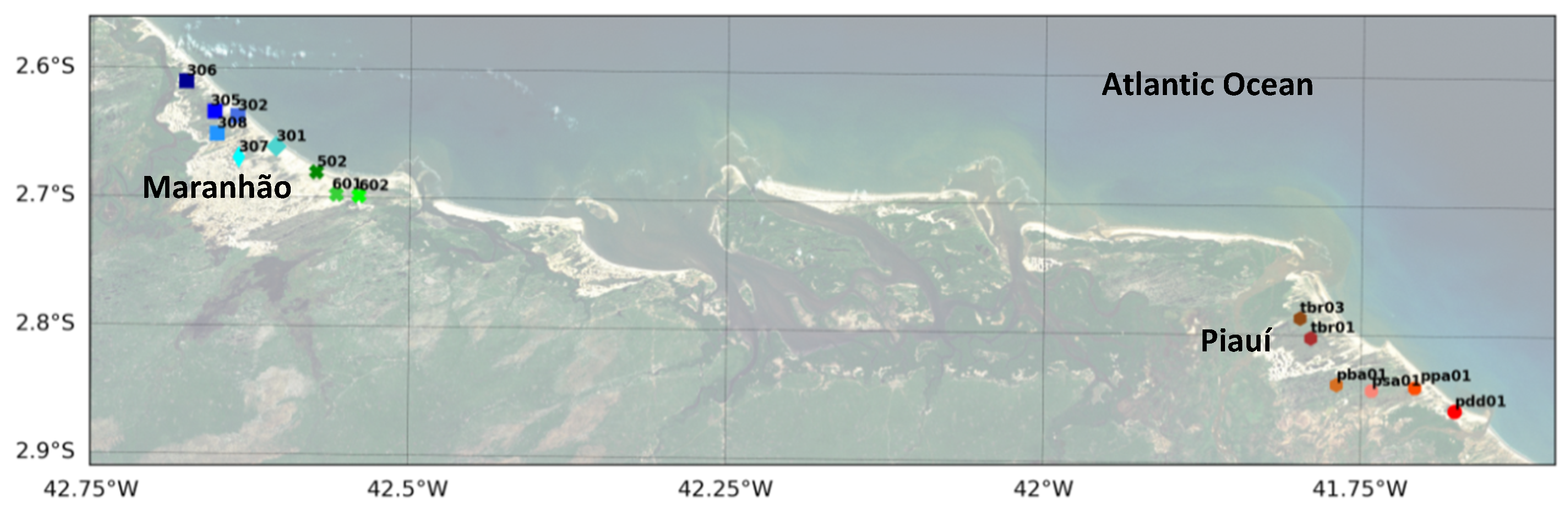
This study was concentrated in the coastal areas of the states of Maranhão and Piauí, in Brazil, illustrated by Figure 2. A total of 25 points of atmospheric measurements were available, containing information of wind, temperature, atmospheric pressure, and relative humidity. After a rigorous quality control [33], a three-year period from 09/2017 to 08/2020 has been selected with high-quality continuous observations available in 16 stations—which were finally selected and shown in Figure 2.
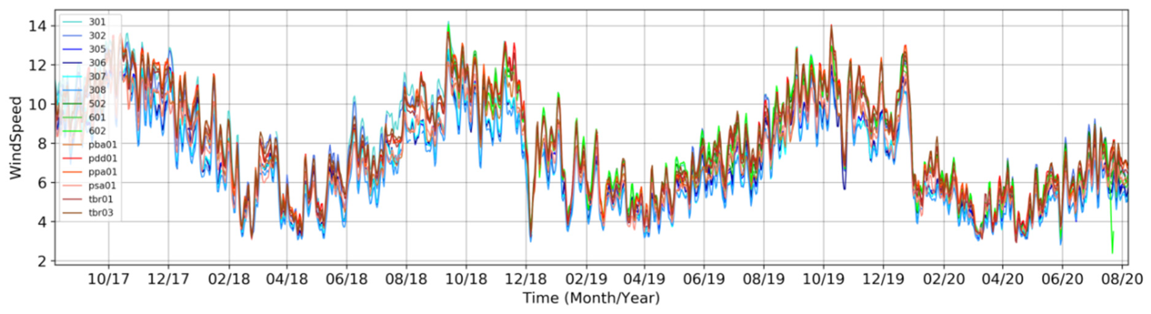
The wind speed was the target variable, the other environmental variables being utilized as additional information for the prediction models. A direct plot of wind speed from all the 16 anemometers is presented in Figure 3, for the three-year period selected. The seasonal cycle is very clear in the region, with higher intensities from August to November (dry season) and lower intensities from February to June (wet season). The wind speeds above 8 m/s from August to November can reach 14 m/s, and during the calm-wind season it varies between 3 to 8 m/s.
The region has no historical records of tropical cyclones, so no extreme events with persistent winds above 15 m/s were found. On the other hand, the continuous trade winds rarely decrease to values below 3 m/s for a long period of time. Figure 3 shows that the seasonal cycle and other oscillations embedded in the time-series follow very similar patterns at all the 16 stations, i.e., despite the local effects, the time-series respond mostly to large scale meteorological systems that affect similarly both states of Maranhão and Piauí. Nevertheless, the wind intensities in the state of Piauí (hot colors in Figure 3) are generally higher than those in the state of Maranhão (cold colors in Figure 3) due to the coastal orientation and orographic effect.
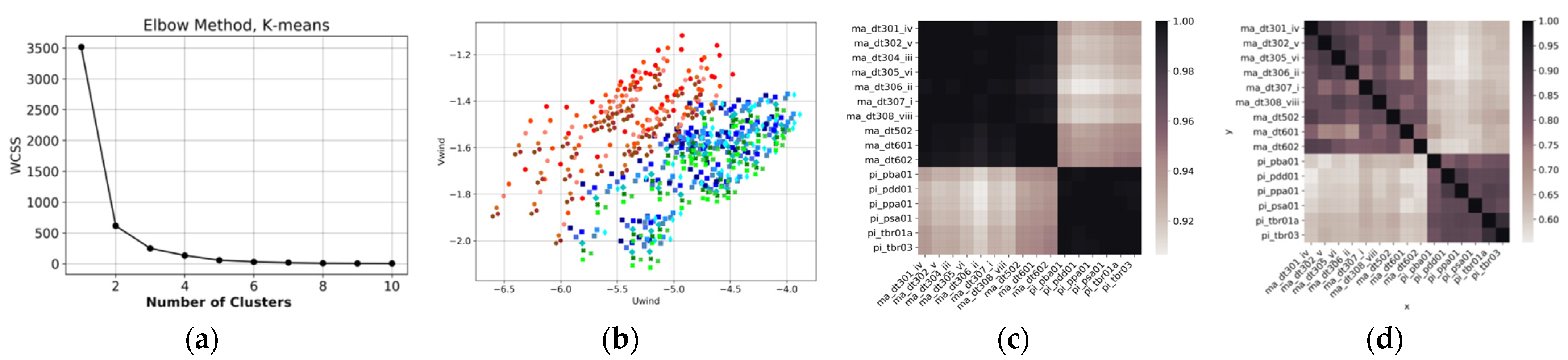
For the model assessments and neural network training, it is important to discuss whether the environmental information at each station will be treated independently or gathered into clusters. This is an important question because the neural network mapping benefits from the inclusion of neighboring points [34], as discussed in Section 4, but the region containing the observations should not be significantly heterogeneous. The K-means cluster analysis applying the Elbow method [35] was adopted to select the optimum number of clusters, where the information of wind ( and components), temperature, humidity, and pressure was included—see Figure 4a.
The goal in the Elbow plot is not to select the minimum value but to identify the “elbow” of the curve, pointing to an improvement in the data clustering while not over-splitting the dataset. Figure 4 shows that two clusters are ideal. Figure 4b presents the plot of the wind components (U and V) for each station, maintaining the color standard of Figure 2 to differentiate the states of Maranhão and Piauí. The separation of two clusters is clear, which is confirmed by Figure 4c,d, where the correlation matrix (Pearson’s correlation and Predictive Power Score) also distinguishes the time-series patterns in two clusters, Maranhão and Piauí. Inside each cluster, the correlations (linear and non-linear) among stations are very high, confirming that the two regions are very homogeneous.
2.2. Global Atmospheric Ensemble Forecast
At forecasting time-scales from 10 to 46 days, as addressed in this paper, the sole use of neural networks with datasets restricted to the stations is unlikely to provide accurate estimates. This challenge is a result of multifactor spatio-temporal correlations that completely change from short-term analysis of a few hours to long-term analysis beyond one month. Souza et al. [36] argue that fluctuations in wind speed in the short range are dominated by atmospheric phenomena governed by local or regional meteorological systems, while fluctuations on long-range time scales are influenced by global weather patterns. The MJO, described above, is an example of phenomena that significantly influences the 30 to 60 days forecasts [37] and requires a global grid modeling to properly represent its generation and propagation. Some very recent studies in machine learning applied to environmental predictions are working on this topic, such as [38,39,40]. However, there is no operational artificial intelligence model so far that simulates the global teleconnections and subseasonal scales with better performance than existing NWP models, for example, those provided by the National Oceanic and Atmospheric Administration (NOAA) and the European Centre for Medium-Range Weather Forecasts (ECMWF). Therefore, including an NWP forecast to build a joint solution of NWP modeling combined with neural networks would certainly improve the predictability at longer forecast lead times. The ECMWF IFS numerical model [41] is coupled (atmosphere/ocean), which benefits the forecast skill at longer ranges, becoming especially important for the present study. The main forecast from ECMWF covers a high-resolution deterministic modeling with a range from 0–10 days and a spatial resolution of 0.1°. The complete list of ECMWF products can be found at: https://www.ecmwf.int/en/forecasts/documentation-and-support (accessed on 1 June 2021).
For predictions involving longer forecast ranges, it is well known [42] that using an ensemble of forecast simulations tends to perform better than single deterministic runs. A traditional approach to ensemble forecasting is to generate several numerical model integrations (members) simultaneously starting from perturbed initial conditions that represent the uncertainties in the initial model state. The straightforward arithmetic mean of the ensemble members has been proven to outperform deterministic simulations (i.e., single control run), as reported and quantified by Campos et al. [43] and Zhou et al. [44]. Kalnay [42] explains that the ensemble members tend to smooth out uncertain components, which lead to better performance than single deterministic forecasts. Therefore, after one-week forecast range, the inclusion of ensemble forecasts is of paramount importance. The drawback of this approach is the computational time dedicated to model simulations, data transference, management, and storage. These limitations explain why ensemble predictions have coarser resolutions when compared to deterministic forecasts.
The ECMWF ensemble is produced with range from 0 to 15 days, and a spatial resolution of 0.2° and 50 members on global domain. Twice a week, an extension of this range is produced [45], covering 46 days of forecast but with a coarser spatial resolution of 0.4°, called ENS-Extended. The model’s implementation utilized in this study (Cy47r1) had its last upgrade on 30 June 2020. More information is described: https://www.ecmwf.int/en/forecasts/documentation-and-support/changes-ecmwf-model (accessed on 1 June 2021).
3. Assessment of the Numerical Ensemble Forecast Data
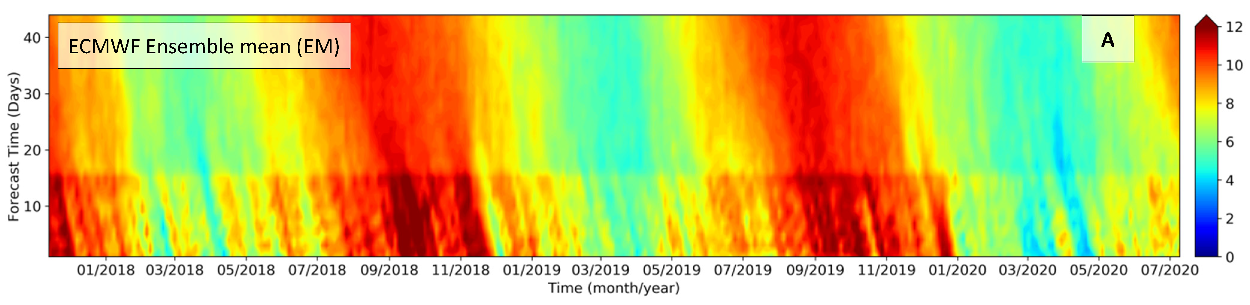
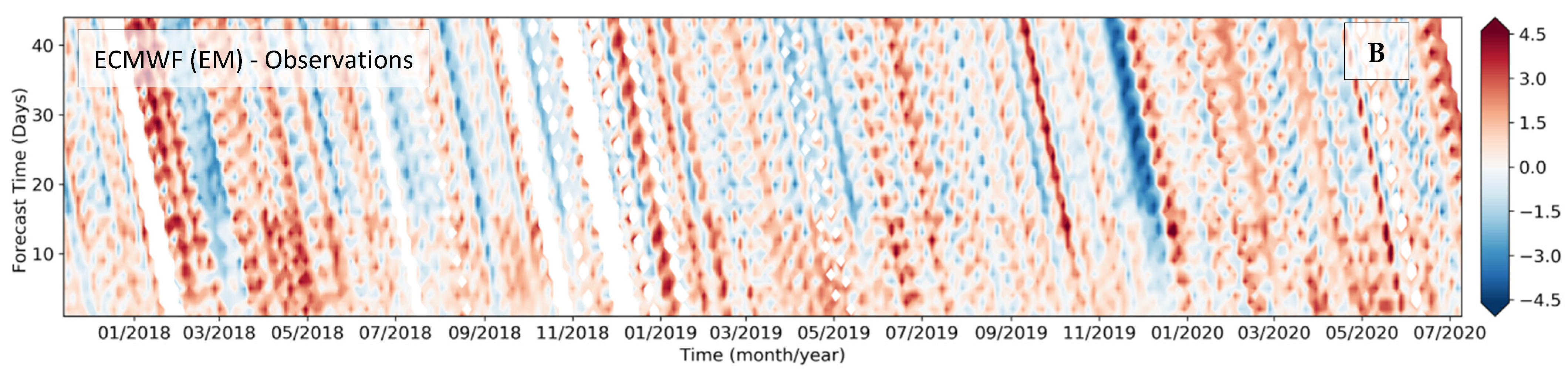
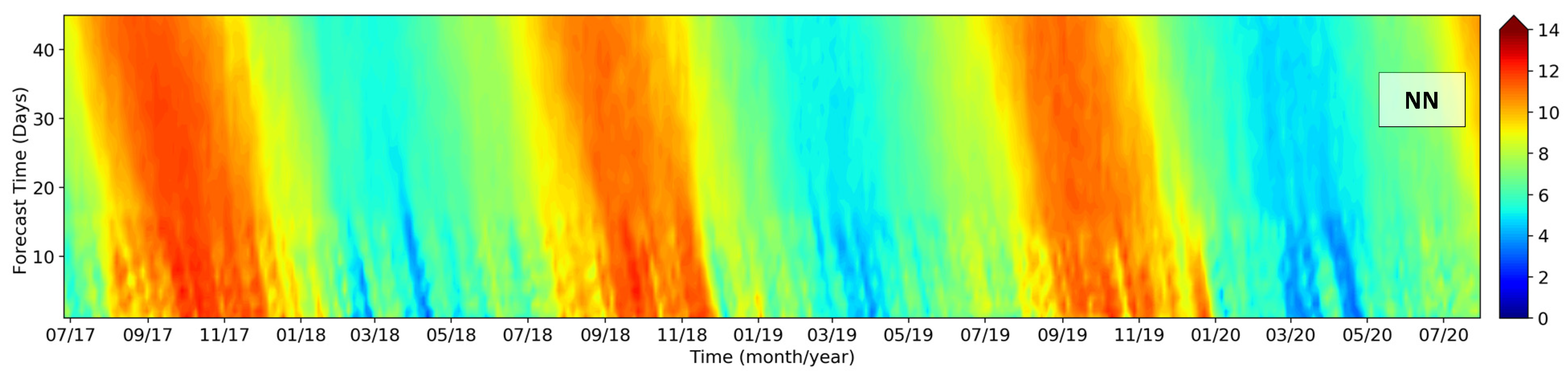
An ECMWF archive of three years of ENS-Extended 46 day’s forecasts was selected for the domain, covering latitudes 40° S to 10° N and longitudes 60° W to 20° W, with a temporal resolution of 3 h. This is the NWP dataset selected for this paper and evaluated in this section. The ensemble point output for the positions of each of the 16 stations (Figure 2) were extracted from this data archive, and paired with the observations (Figure 5)—this allowed a complete assessment of the ensemble followed by the construction of post-processing neural network models. This ensemble dataset consisted of an array of 16 points containing three years of forecast cycles (twice a week, on Mondays and Thursdays), each one with 46 days of forecast lead times. By simply selecting one of these points, and plotting consecutive forecast cycles (x-axis) with the forecast lead time on the y-axis, it is possible to build a matrix containing the entire forecast for each point. Figure 5A shows an example for a station in the state of Maranhão, where the direct difference (model minus measurement) is plotted in Figure 5B.
The graphics of Figure 5A are very rich, illustrating several features in the same plot. Firstly, it is possible to confirm the seasonal cycle with strong winds from August to November and light winds from February to June, proving that ECMWF simulations agree with observations for this time scale. Secondly, the effect of resolution is seen through the discontinuity in the wind intensity on the y-axis, where the first 15 days (0.2° of spatial resolution) have stronger winds than the forecast ranges from 16 to 46 days (0.4° of spatial resolution). Figure 5B shows accurate forecast instants in white color, which are typically found during the first forecast days (lower y-axis values) close to the analysis (nowcast, y = 0), progressively growing at longer forecast lead time due to the chaotic component of the atmosphere. However, the “stripe” shape of Figure 5B suggests that specific events of intensification and attenuation of wind speeds tend to loose predictability, showing poorer skill, and such lower model performance tends to remain similar towards the forecast time—i.e., when an oscillation in the wind intensity is not properly modeled, this tends to remain inaccurate throughout the whole forecast range. Such a characteristic revels two important points: (1) the numerical model and its resolution cannot properly simulate certain types of events and (2) the overestimation of winds tends to be followed by underestimation at scales of 10 to 50 days, and this error is not solved even at short forecast ranges. Lee et al. [46] and Camp et al. [47] discuss the challenges of subseasonal to seasonal (S2S) atmospheric forecasts in tropical areas.
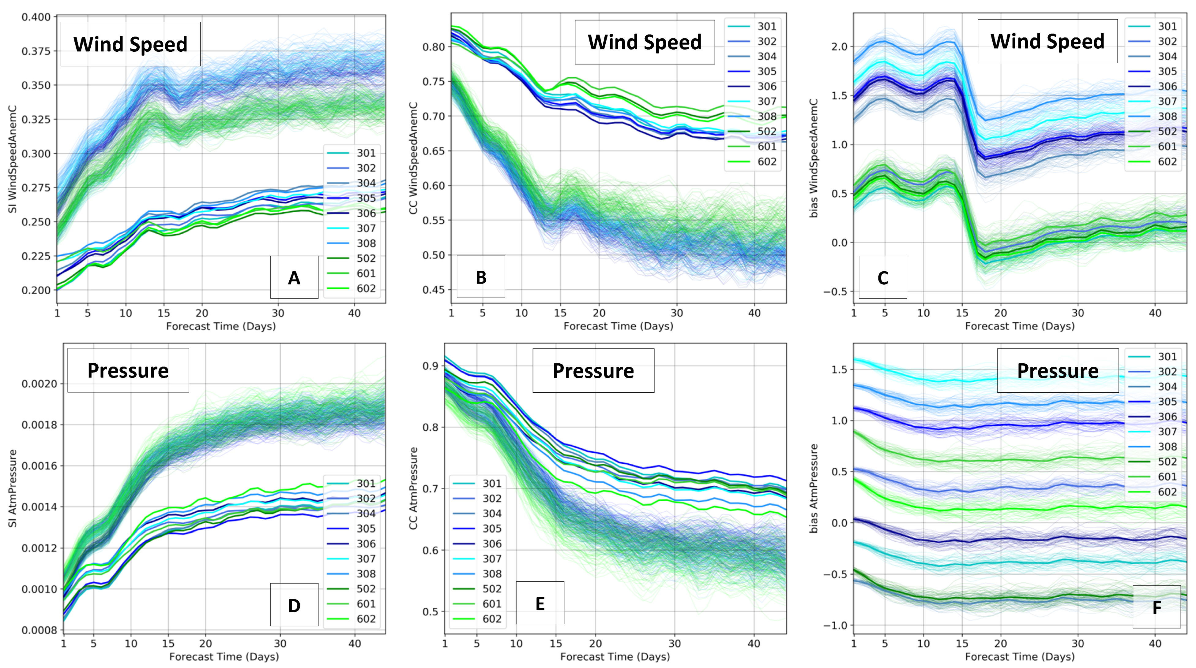
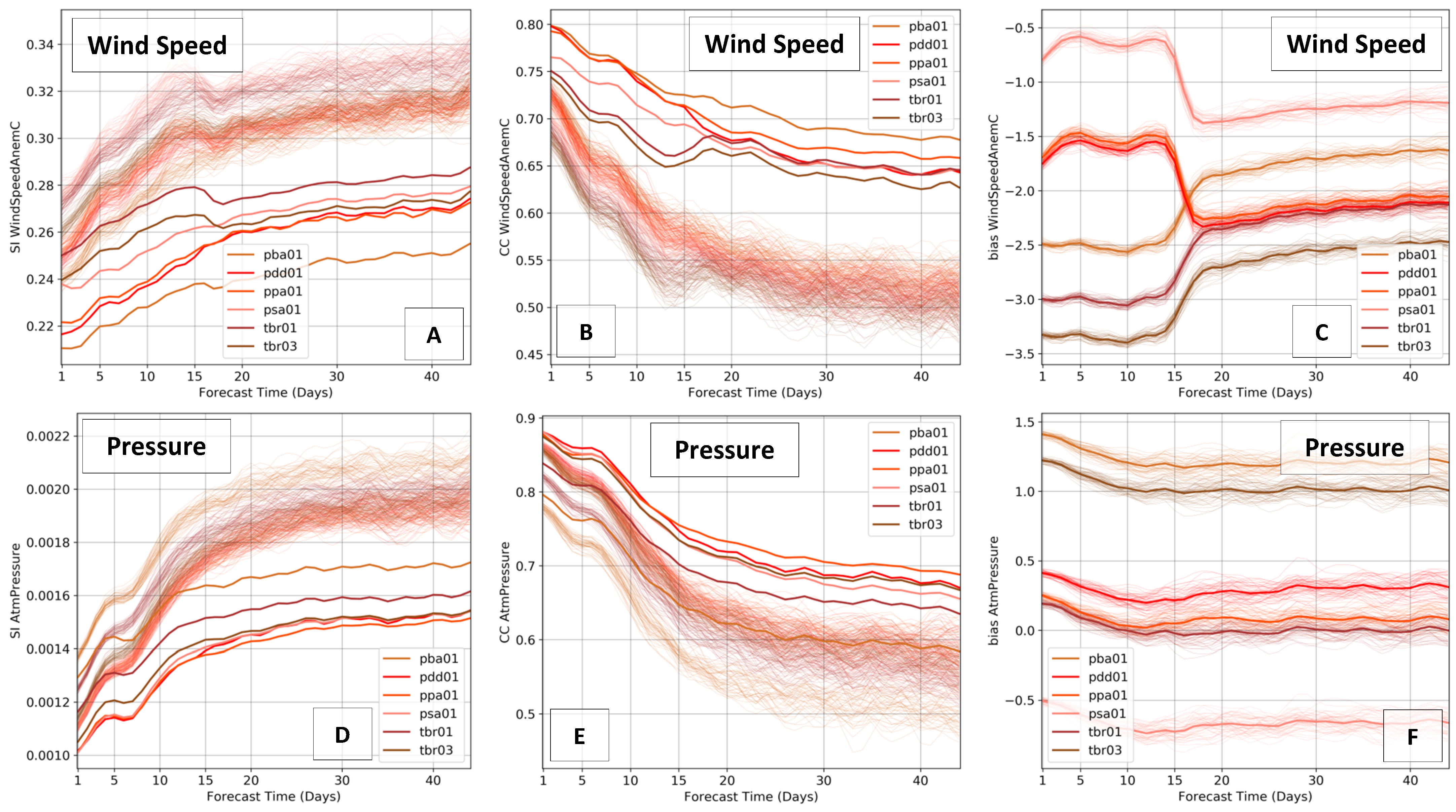
In order to provide a complete assessment of the ECMWF ensemble forecast, four error metrics were calculated as a function of the forecast lead time at each station. Equations (2) to (5) describe the metrics, where are the measurements and the ECMWF forecast, and the overbar indicates the arithmetic mean. The systematic and scatter errors of the forecasts will be extensively discussed in this paper using the bias and scatter index, respectively. The scatter index can be interpreted as a percentage error when multiplied by 100. Typically, the pattern of lack of predictability at longer forecast leads is visualized by the increase of SI and the decrease of CC—the two most difficult metrics to improve. The next Figure 6 and Figure 7 show the results for each cluster, for wind speed and atmospheric pressure at mean sea level.
Figure 6 and Figure 7 have common features that illustrate the general characteristics of the atmospheric modeling, such as the rapid increase of SI and decrease of CC in the first 15 forecast days. After this range, from 20 to 46 days, errors tend to be more stable and very large. Additionally, both clusters show better performances for the arithmetic ensemble mean (EM) of the ensemble members when compared against the individual members. This difference is less evident at the analysis (nowcast) but it grows as the forecast lead time increases, confirming the importance of the ensemble approach at mid- and long-forecast ranges. Such an effect is found in the SI and CC but not in the bias, where the error of EM and individual members are very similar. Therefore, the systematic errors are not reduced by the ensemble approach, which requires post-processing bias-correction tools.
In Maranhão, the SI of wind speed varies from 20 to 28% for the EM and from 24 to 38% for the single members. The CC at the same state varies from 0.83 to 0.65 for the EM and from 0.75 to 0.50 for the single ensemble members. The results highlight again the differences between the ensemble forecast and deterministic runs. In Piauí, there is more dispersion among the stations inside the same state, especially in the first 15 days. The SI of wind speed varies from 21 to 29% for the EM and from 24 to 34% for the single members. The CC varies from 0.8 to 0.63 for the EM and from 0.73 to 0.42 for the single ensemble members.
Regarding the systematic errors, note the differences between the two clusters, reflected in the bias plots of Figure 6C and Figure 7C. In Maranhão, bias is mostly positive, reaching 2 m/s within the first forecast days—which indicates that ECMWF forecast winds are more intense than measurements (model overestimation). However, in Piauí, where the winds have been shown to be more intense than in Maranhão, the bias plot has negative values, i.e., the observations are more intense than ECMWF forecast winds (model underestimation). This feature suggests that the NWP global simulations from ECMWF ENS-Extended tend to provide similar wind intensities in both states, while the observations prove they are significantly different, with Piauí containing stronger winds. Therefore, despite the quality of the ensemble forecast, the local characteristics and differences of surface winds in the northeast of Brazil are not properly simulated.
Another important limitation of the extended 46 days ensemble forecast can be found in the evolution of the error metrics throughout the forecast time, passing from day 15 to 16. The wind errors, in both states, show a very large jump at this boundary after 16 days, which reflects the different resolution of the model, from 0.2° to 0.4°—already found in Figure 5. The higher resolution in the first 15 days provides stronger winds than the coarser resolution from days 16 to 46—clearly visualized in the bias plots. By analyzing the entire forecast range from 0–46 days, this problem becomes more critical, since the lower wind speed values, due to the model’s resolution, can be interpreted as a light wind period approaching. Interestingly, such strong discontinuity found in the wind errors is not present in the atmospheric pressure (hPa) error plots. The CC of pressure, for example, smoothly decays with increasing forecast days. The bias plots reinforce this feature, where the errors are nearly constant for the pressure. It is possible to conclude that the ECMWF ensemble forecast provides quality predictions of surface pressure, which responds to large-scale atmospheric phenomena, whereas the surface winds suffer from errors due to the influence of regional scales that require higher resolution and proper physics.
Therefore, for the post-processing algorithm to be attached to the output of the ensemble forecast, it must be able to bias correct the ensemble mean of the wind speed by learning the local characteristics from measurements, while still preserving the proper large scale prediction coming from the NWP model.
4. Neural Networks for Post-Processing
The neural network (NN) model selected for post-processing the ECMWF ensemble forecast was a Multilayer Perceptron Neural Network (MLP-NN, [26]), which is a simple and powerful nonlinear mapper suitable for operational applications. A complete theoretical description is provided by Haykin [48] and several applications in environmental sciences are found in Krasnopolsky [49]. Samet et al. [13] confirm that MLP-NNs are widely utilized in wind forecasting applications.
The MLP-NN is a feed-forward artificial NN that uses supervised learning, containing three or more layers: one input layer, one or more hidden layers, and one output layer. The next equation (6) presents the model, where are the inputs, the outputs, and and are the model parameters to be optimized. The total number of inputs and outputs are and , respectively. The first summation represents the “neuron” of the network, with the activation function hyperbolic tangent (), where is the total the number of neurons. Among the many activation functions available, have shown very good results while still preserving the simplicity, as its derivative .
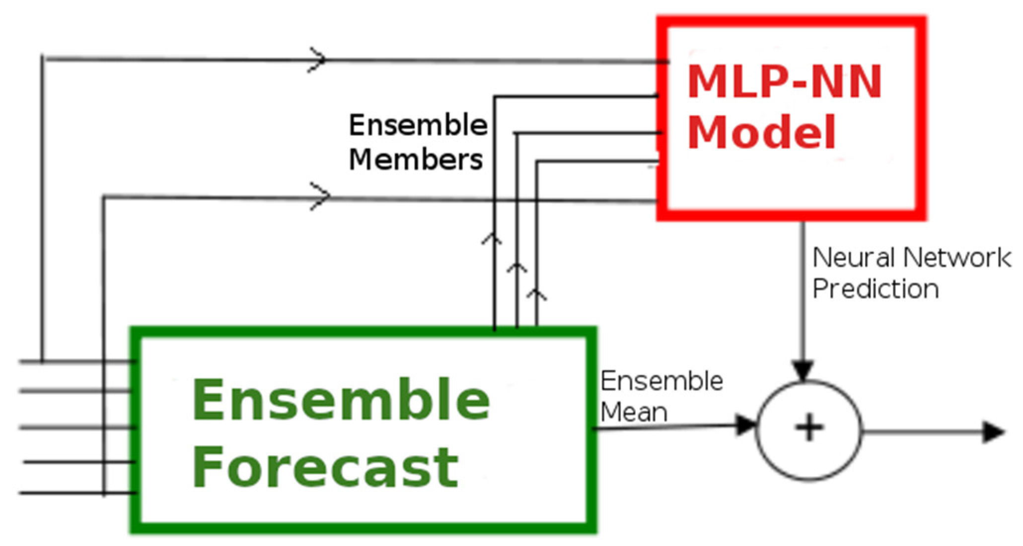
The optimization of and was done with backpropagation training using gradient decent. In fact, it has been found that the stochastic gradient decent that evolved to the adaptive moment estimation (ADAM) described by Kingma and Ba [50] provides better results and thus it was the method selected for this study. ADAM is especially suitable for sparse gradients and variables with strong noise components, which is the case of the environmental problem of this paper. Inspired by [34,51], the target variable of the MLP-NN model is not directly the wind speed but the residual, i.e., the difference between the ECMWF forecast and the observations—illustrated by Figure 8. Therefore, the NWP modeling from ECMWF provided the ensemble mean as the first outcome that was directly compared and subtracted from the local measurements to build the residue signal. When the hybrid model is running, the ECMWF provides the EM that is added to the residue forecasted by the NN, to finally compose the forecast of wind speed. Due to the chaotic process of the atmosphere and lack of high-frequency predictability after two weeks of forecast [52], the daily average was used in the hybrid model—which avoids the excess of noise that contaminates the model.
At this stage, it is important to discuss the construction of input and output dataset for training. The data structure is represented by , described below, containing variables coming from the ECMWF forecast (wind, temperature, humidity, and pressure) and records (or quality-control measurements selected). In fact, the decision of is more complex due to the two additional dimensions associated with the forecast lead time and several stations (positions) inside each cluster.
The NN prediction for each forecast lead time can be done independently, building one NN per forecast time, which would preserve the space but it would increase the number of NNs—leading to a cumbersome operational system. On the other hand, a new variable containing the information of forecast horizons (1 to 46 days, once daily averages have been used) can be added to the NN, concatenating the forecast dataset into a new column and increasing , related to the number of lines of . Hence, the new space becomes , where all the forecast times are appended into the NN and, therefore, one single NN model can predict different forecast leads—which has been the approach selected for this study.
Similarly, the spatial modeling for each cluster (Maranhão and Piauí) leads to three options in the NN:
- (i)
- Build one NN for each station, independently. Therefore, the datasets of neighboring stations are not included into the NN training and modeling, i.e., the inputs (ECMWF forecast) and outputs (residue of wind) are restricted to that specific station.
- (ii)
- Build a large NN where inputs are the information from all the stations inside the cluster (10 for Maranhão and 6 for Piauí) and the outputs are the residues of wind speed for the same stations. In this way, the dataset is expanded in , where corresponds to the environmental variables at each station. The data space for this approach, for example at Maranhão with 10 stations, would be .
- (iii)
- Build one NN where inputs and outputs are variables for each station, which are one by one appended to generate a new dataset, where two new variables’ latitude and longitude are included to distinguish the stations. In this case, the training consists of an NN model passing through each station inside the cluster during the process. Note that the training data is constructed by appending the dataset of each station consecutively, so that the NN minimizes the error at the whole group of stations. Following the same example at Maranhão with 10 stations, the new space becomes . It is important to highlight that in (ii), the number of input variables and dimension is significantly augmented (10 times in Maranhão), whereas in (iii), the number of variables is just , while the number of records is significantly expanded—following a similar approach of space/time trade proposed by the regional frequency analysis [53].
There are pros and cons in each option described above. The first option (i) is the worst strategy because it ignores the neighboring data that could help improve the optimization, wasting the opportunity to increase the training dataset. The second option (ii) has the benefit of joining all the information inside the cluster. However, by appending the columns with several stations (increasing ), if one station has missing data, it compromises the entire record , which means that only instants when all the stations have quality measurements could be used as training records. It is well-known that observations often suffer from outliers and wrong data that are excluded in the quality control process, as well as the initial/final dates of data collection can differ from one station to the other, thus limiting the final number of days used for training. Moreover, higher dimensions usually require larger networks with more neurons, as described by Krasnopolsky [49], which also demand more data for training. Therefore, expanding while maintaining is actually the opposite of what a good strategy should consider. Additionally, the NN structure of (ii) only allows the model to make predictions for the specific stations utilized for training, i.e., if one new station is included in the future, the model must be re-trained, and the new point can only be included when gathering enough duration to time-match with other stations and provide a sufficient coincident period of time for training.
The third approach (iii) combines several advantages and thus has been selected for the NN model implementation. The first and most important is the option of including all the stations for NN training no matter the duration of measurements or data gaps. By training the NN model at different stations with information of latitude and longitude, the NN performs a spatial mapping (position becomes a new dimension), so whenever new points are included in the future, the existing model can directly generate forecasts for these new positions. Furthermore, the new points with recent and short data collection can also be included in the NN re-training without having to modify the data structure or number of input/output variables. Therefore, each station bringing its measurements to the NN training contributes to the regional modeling by inputting short-scale information and improving the resolution at the region. Another important advantage of (iii) is that the NN preserves a small dimension () while increasing the data records for training during the process of appending all the stations into a single dataset. In summary, latitude and longitude are two dimensions for spatial modeling, and time and forecast lead time are two additional dimensions as well. This data structure and training strategy was conceived by Dr. Vladimir Krasnopolsky in [34], which allowed the successful construction of a global NN model in [51].
In practical terms, two separated NNs were built and trained for each cluster (Maranhão and Piauí) and, due to the effect of predictability profile and model resolution on the wind forecast and intensity, it was decided to separate the 46 days of range into two slices of 1–15 days and 16–46 days. Therefore, four NNs were developed to cover two forecast ranges and two clusters. The last step was to include the methodology proposed by Krasnopolsky and Lin [54], who argues that an ensemble of NNs outperforms single NN models alone. The NN ensemble construction can be easily implemented by managing the random initialization of and through the “seeds”. It is possible to generate several -independent NNs with different random initial conditions and, as proven by [15,54], the arithmetic mean of results provides better prediction than using a single NN alone. Additionally, the spread of those predictions provide information of uncertainty in the forecast, similar to what is traditionally evaluated in NWP models. Moreover, by generating a large number of NNs, it is possible to exclude the networks with poorer performance and pick only the networks with the best results. This methodology has been implemented for the NN modeling so, in terms of outputs, the schematic of Figure 8 can be expressed as:
where EM is the ECMWF ensemble mean and is the arithmetic mean of networks with parameters . The result of the hybrid system, , is the final wind forecast.
Expanding the discussion of dimensionality of the NN model and training data, but now focused on the input variables with meteorological information, it is crucial to investigate how the ECMWF outputs will feed the NNs. Being an ensemble with 51 members (50 perturbed members plus the control) and considering the variables wind ( and components), pressure, temperature, and humidity, the number of environmental inputs for the NN reached 255. Zaki and Meira [55] reinforce the challenges and possible problems involving high dimension, which is especially critical in operational applications that require reliable and robust models. Thus, a feature selection was conducted to: (i) analyze the importance of each component of meteorological information (wind, pressure, temperature, and humidity) and how this inclusion/exclusion affects the performance of the model, first in the input and then in the output;(ii) analyze if the 51 members are necessary as inputs or if it is viable to replace them by their probabilistic moments (mean, variance, skewness, and kurtosis), such as applied in [34,51]. It was found that including all the 51 members significantly increases the number of inputs which demands larger NNs, which lead to training difficulties. In practical terms, the performance in the training set was satisfactory while in the test set it was compromised. Consequently, it was safer to move forward with the probabilistic moments, since these captured the characteristics of the 51 members while reducing the number of variables.
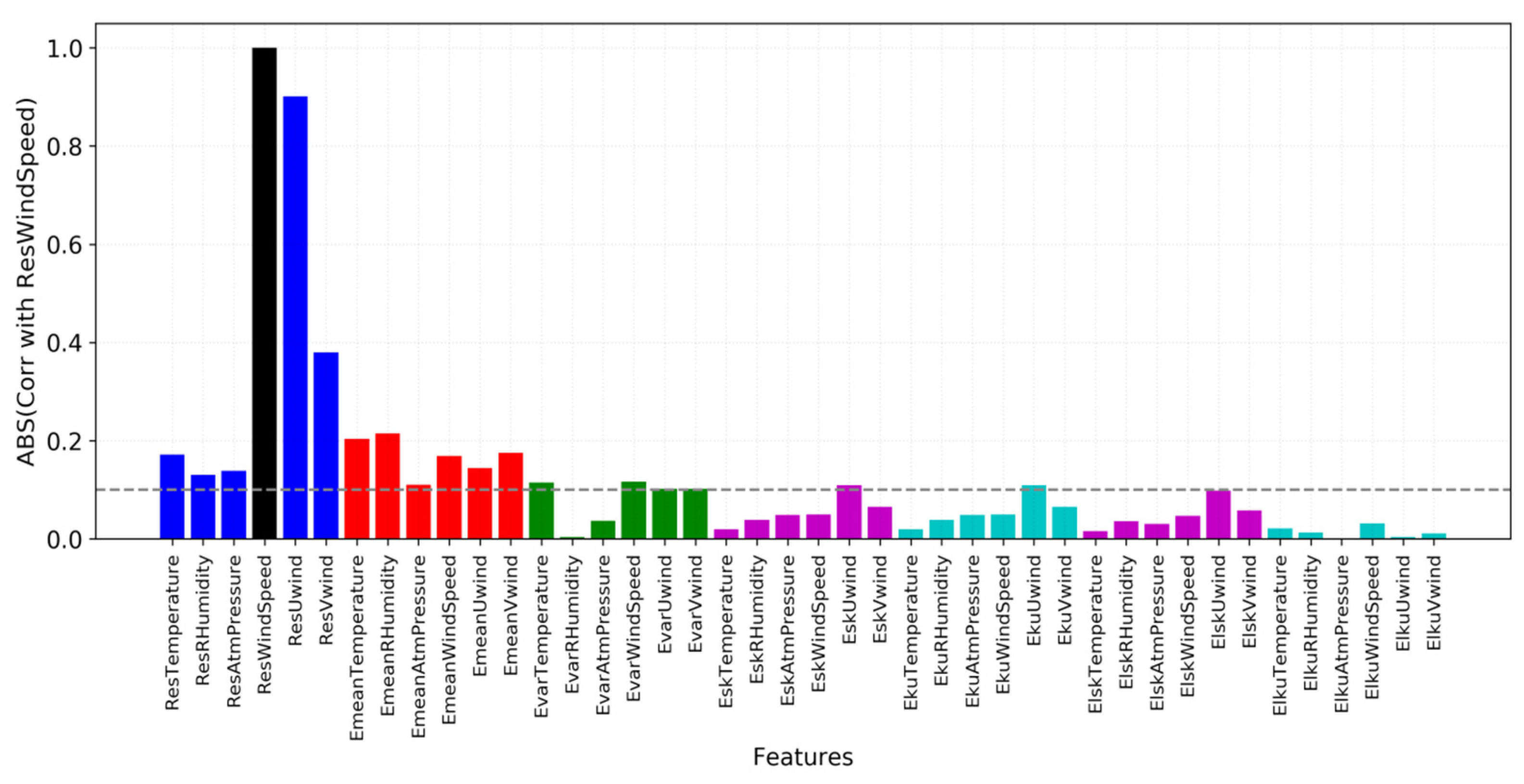
The next Figure 9 illustrates part of the feature selection process, where the importance of each probabilistic moment from each meteorological variable relates to the target variable (residue of wind speed, in black in the figure). The feature analysis takes into account the Pearson’s Correlation and the Predictive Power Score. Besides the straightforward probabilistic moments, the L-moments [56] were included, due to being less affected by outliers in the time-series. Figure 9 shows a nearly equal importance of temperature, humidity, and pressure into the outputs. Regarding the inputs, the first moment (mean) shows a greater importance of humidity and temperature, and lower importance of atmospheric pressure. This pattern completely changes for the second moment (variance), where humidity loses its relevance. Moving to higher moments, the impact of variables drops significantly but the zonal () component of the wind remains important. Nonetheless, when the skewness of the ensemble members is different than zero (asymmetry), it can provide valuable information, once it directly affects the ensemble mean—a common effect at longer forecast leads. Figure 9 and later results indicate that L-moments do not contribute to the NN modeling when compared to the standard probabilistic moments.
The feature selection algorithm initially applied a methodology inspired by [57,58], followed by the analysis of all the combinations of input and output variables, evaluated in both clusters and through the 46 days of forecast range, considering the performance in the training and test/validation sets. The best combination of variables gathered for inputs was the ensemble mean (temperature, humidity, wind speed), variance (temperature, and and wind components), and skewness (humidity, and and wind components). For outputs, this was the wind speed, accompanied by the meridional component of the wind only. This gave 10 environmental variables for the inputs, which also included the forecast time, sine and cosine of time (to properly identify the time of the year and differentiate seasons), and latitude and longitude—a total of 15 inputs. The number of outputs was two.
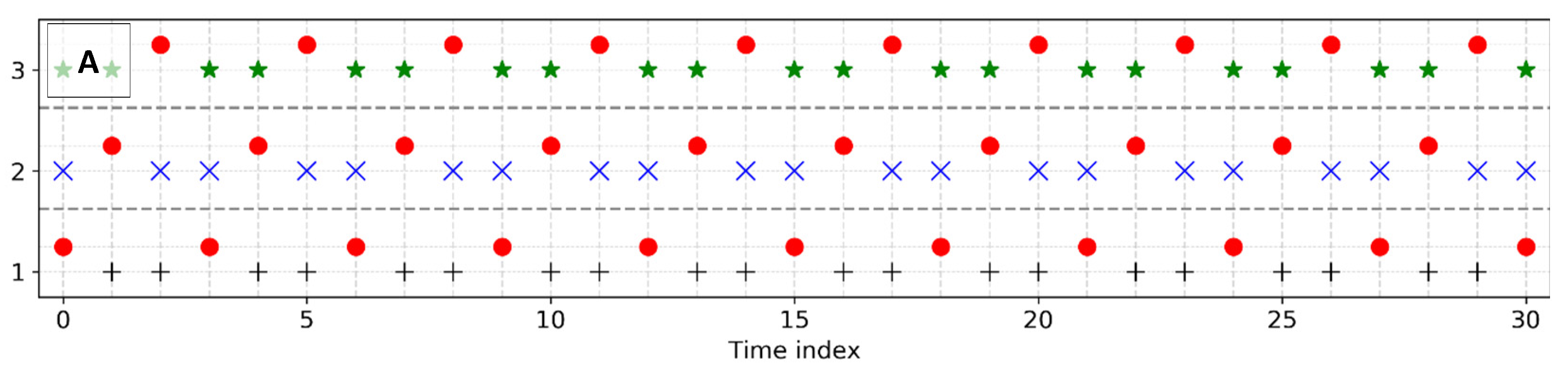
The NN training as well as other tests involving feature selection, optimization of the number of layers and neurons (next section), and evaluation of final results were carefully conducted with a proper data division into training set, test set, and validation set. The most basic requisite was to train the NN model using records that were not selected for testing. The leave-one-out cross validation method with three cycles (Figure 10A) was implemented, where two thirds of the dataset was used for training and one third for testing the network—with intercalated indexes that can be joined to reconstruct a test time-series with the exact same time as the original one. However, such a method carries a limitation of building training and test sets within the same time interval, i.e., both sets correspond to the same atmospheric conditions inside an ergodic system.
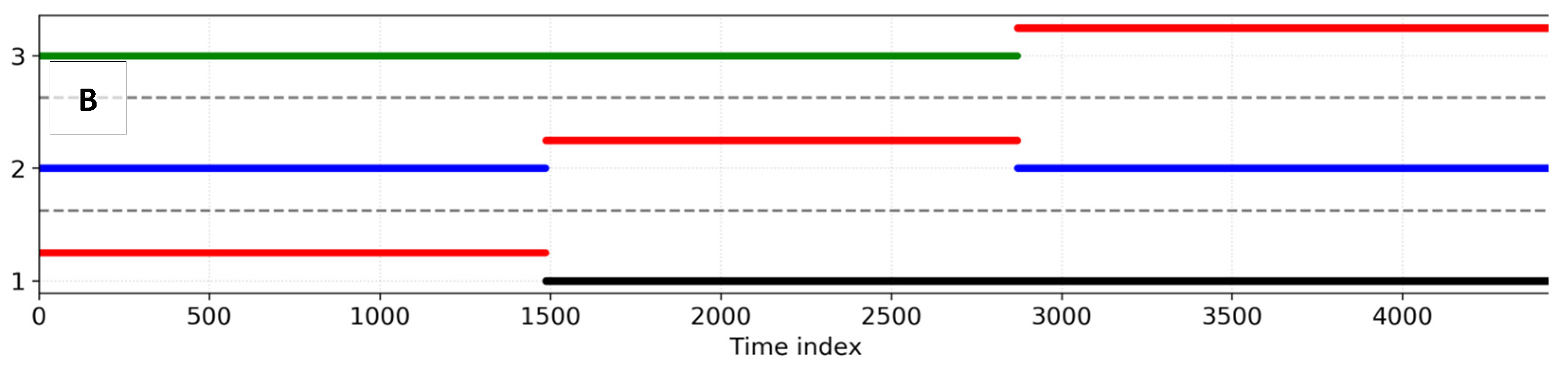
It is extremely important to evaluate the NN considering a different time interval and atmospheric conditions, in order to evaluate the extrapolation and generalization of the model—which is critical for operational implementation. Therefore, a validation set was built (Figure 10B), where the NN was trained and tested using two years of data, and validated using a separated year. This strategy allowed for the simulation of a real forecast in operation, for when the NN cannot be constantly trained. In reality, the validation set evaluates the extreme scenario of not re-training the NN model for an entire year—which is not necessarily the real case with the NN being re-trained at least twice a year. The total number of records in this three-year period was 46,656, which were used for the model optimization and evaluation as explained. Therefore, the total input dimension was 46,656 × 15 and the output dimension was 46,656 × 2.
5. Results
The NN methodology described in the last Section 4 proposed a relatively small network with 15 inputs and 2 outputs, using a simple model such as the MLP. This is a key strategy to allow training many NNs for each cluster, in order to build a final ensemble of NNs. If a large and complex model had been developed, the ensemble approach would not be viable under the computational infrastructure available. The remaining questions are how many neurons at the intermediate layers are optimal and how to select the best networks to compose the ensemble.
5.1. Neural Network Architecture and Ensemble
A combination of different numbers of neurons () have been tested within one and two intermediate layers: [5, 0], [10, 0], [20, 0], [50, 0], [100, 0], [150, 0], [5, 5], [10, 10], [20, 20], [50, 50], [100, 100], [150, 150], where the two numbers inside brackets are related to layers. Therefore, 12 different NNs were tested, each result being the average of 5 NNs with different random initial conditions, composing a total of 60 NNs. All networks, even the simplest ones, showed to be successful in reducing the systematic errors, with bias close to zero—as expected. The differences between NN models were more evident when SI and CC were analyzed. The next Figure 11 shows the effect of different numbers of neurons into the two metrics, for the training and test sets, using one intermediate layer initially. The results point to the optimum number of 20 neurons, the region between 20 to 60 neurons having the best performances. Above 60 neurons, the scatter error increases and the correlation decreases, i.e., more complex NNs do not necessarily improve predictions.
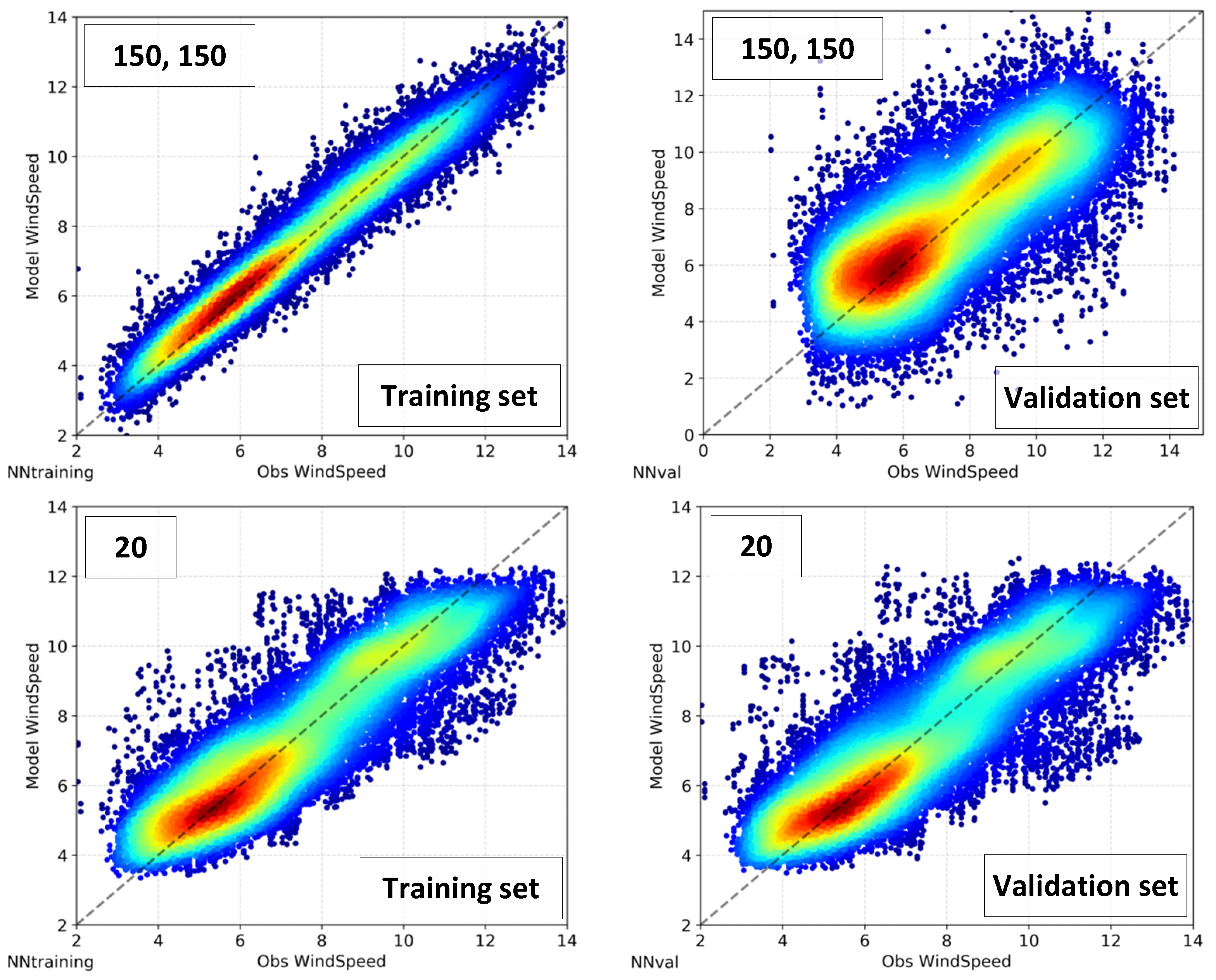
Increasing the number of neurons through the second layer severely compromised the test and validation sets. Figure 12 is a good example of the impact of the NN’s complexity on different sets. The figure shows scattered plots integrating the whole range of forecasts, for the three-year period. Ideally, a perfect result should follow the principal diagonal with the least spread as possible. When the most complex model with two layers containing 150 neurons was compared with the optimum model with one layer containing 20 neurons, for the training set solely, one could conclude that the larger NN performed better. However, when the scatter plot of validation set was included, it is clear that the lack of generalization and poor extrapolation severely deteriorated the NN simulations. The simpler NN with 20 neurons, on the other hand, preserved very similar results in both sets—which ensures better forecasts under operational use. It is important to remember that the goal of the NN model is to either improve or to preserve the ECMWF forecast performance. A post-processing NN model that adds error to the existing NWP forecast would be detrimental and therefore unacceptable.
The small number of NN inputs and outputs combined with the optimum number of neurons equal to 20 allowed the allocation of hundreds of NNs for training. Moreover, having spare computational resources gave the opportunity to include additional experiments related to the seasonality. As described in Section 2.1, the northeast of Brazil has two very distinct seasons: a dry season with strong winds and a wet season with calm winds. Considering that NNs perform better within homogeneous datasets under minor extrapolations, the new tests consisted of training NNs for specific seasons. Therefore, instead of one NN for the entire period, three NNs were used: one for the strong-wind season (SWind, from August to December), one for the light-wind season (LWind, from February to July), and the last one preserving the original NN for the whole period (all-year, AY). Such an inclusion made the initial four NNs (Maranhão/Piauí, for the forecast ranges from 1–15 and 16–46) become 12 NNs, with the addition of seasonal tests; evaluated in Figure 13.
A total of 201 different seeds initialized the networks, for each of the 12 experiments, which led to 2412 NNs being trained and evaluated. Figure 13 shows the results of the three-year period, where the error metrics were calculated for each month of the year to compare the NNs and the performances throughout the seasons. The ensemble mean from ECMWF is included as reference, to highlight the NN models that are better/worse than the ECMWF ensemble. The NNs trained for specific seasons were run for the whole year, on purpose, to evaluate the NN application under completely different environmental conditions used for training. As expected, the quality of the seasonal NNs was good only when applied for the season it had been trained for. However, the characteristics of deterioration of these NNs are very important to be investigated. As shown in the figure, the error largely grows followed by the increase of the spread of the 201 NNs. On the other hand, when the NN is performing well, the spread among NNs is very small and the simulations are very similar. This result suggests that the NN architecture, when developed, combined with the ensemble approach, will indicate future loss of predictability when applied operationally in real time, which is a strategic advantage of great value.
Surprisingly, the seasonal NNs operating for the same months they were trained did not over-perform the all-year NNs. One explanation is the amount of data selected for training. When seasonal NNs are trained, the total dataset is subsampled to fit into that time range, which reduces the number of records. As NNs depend on large datasets for proper training, the NNs using the whole three-year period took advantage of the larger amount of data. Moreover, the NN input variable containing the time information allows the network to identify the meteorological patterns at each month of the year and, combined with all available measurements for training, produced the best results. Figure 13 shows that all-year NNs have very low errors in every month, being always lower than the ECMWF reference. The general error profile indicates the lowest values of RMSE during the strong-wind season in Maranhão, and between May to August in Piauí. The variation of monthly errors is more pronounced in Piauí than in Maranhão.
Based on previous results, it was decided to choose the all-year NN strategy, in blue at Figure 13. However, the plot still shows 201 NNs per cluster, a high number of networks that is not necessary for the ensemble composition, and which could add computational time plus data management difficulties during the operational application. Therefore, a 20-member NN ensemble was proposed. A new algorithm was designed to source 20 NNs out of the 201 networks available, based on a ranking composition using the error metrics (Equations (2)–(5)) together with additional exclusion criteria. Since bias is a metric that nearly all the NNs are very effective in reducing, it was used as an excluding criteria and not selected for the ranking composition; otherwise, a small difference of for example 0.0001 m/s would exclude certain networks, while the scatter error, correlation coefficient, and robustness throughout the months are more important criteria. The ensemble composition algorithm does not consider the assessment in the training set, only over the test and validation sets, through the weighted average . The algorithm follows the steps:
- The NNs with normalized bias above 10% are excluded, including the mean value (through forecast range) as well for each forecast lead time.
- The NNs with bias or RMSE worse than the ECMWF ensemble forecast are excluded, i.e., no NN model can risk deteriorating the original ECMWF prediction.
- Additionally, the algorithm analyzes each month of the year, excluding NNs with bias and RMSE worse than ECMWF.
- The algorithm runs the error metrics through the forecast lead time (1 to 46 days) excluding the worst NN at each forecast lead (day), which prioritize networks more consistent over the months.
- The last monthly swap is done at this stage, excluding the single worst network at each month.
- After the exclusions of steps one to five, the algorithm takes the remaining networks and builds two ranks with the best SI and CC, calculating the intersection of the two lists. The top 20 networks are finally selected to compose the ensemble of NNs.
This methodology was conceived to be applied to other applications and NN ensembles, not only to the wind forecast of this paper. The results of the modeling are composed of the arithmetic ensemble mean of the 20 NN members, for each state (Maranhão/Piauí) and forecast range (1–15 and 16–46 days).
5.2. Evaluation of Results
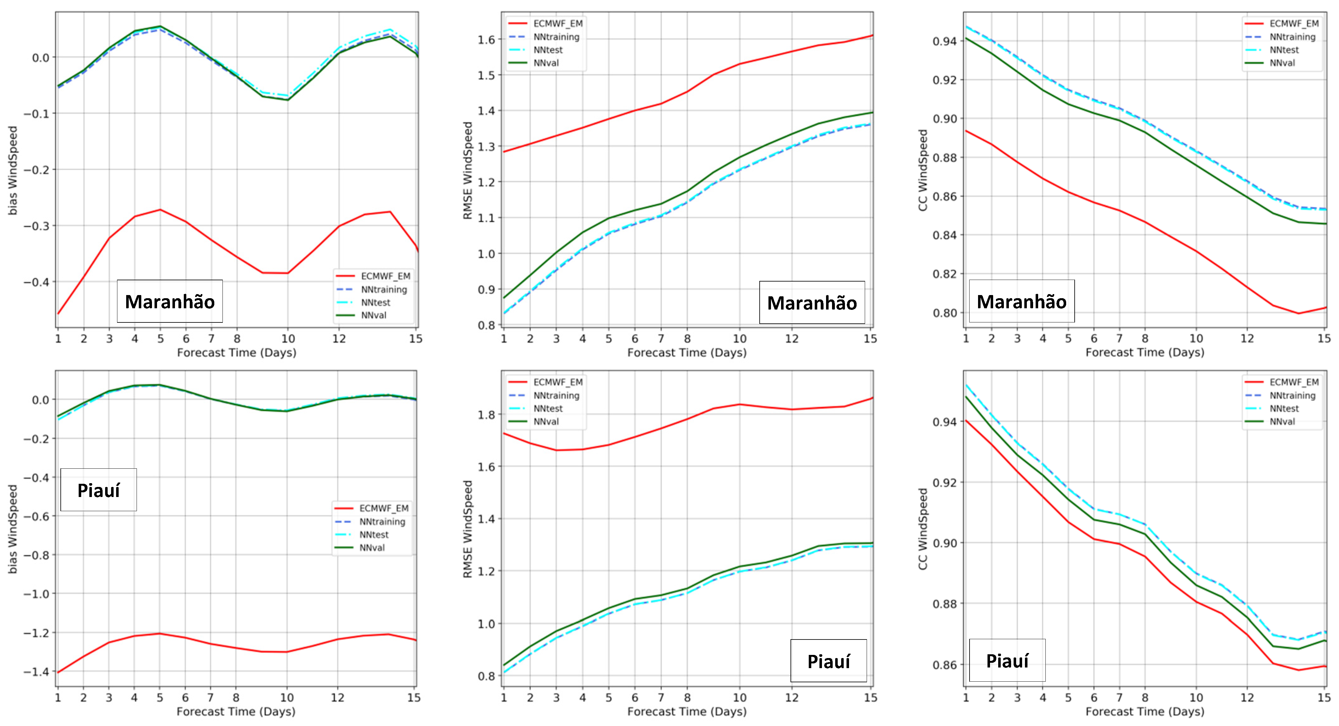
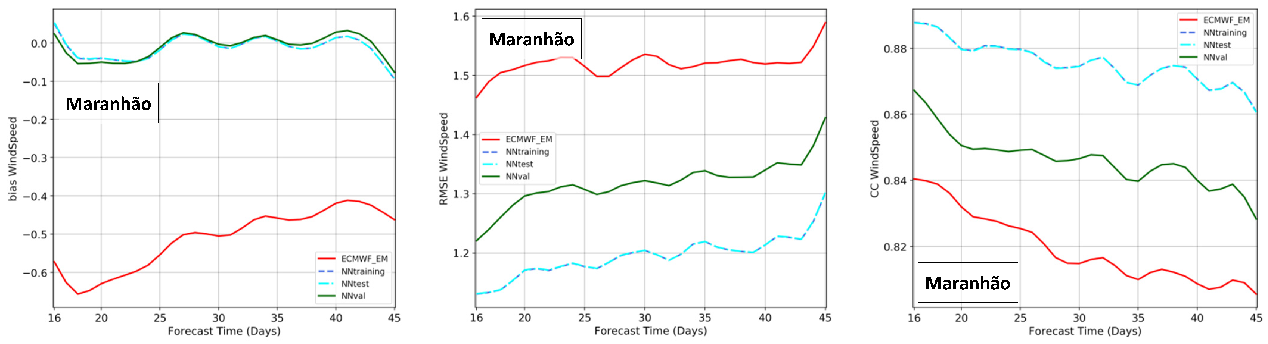
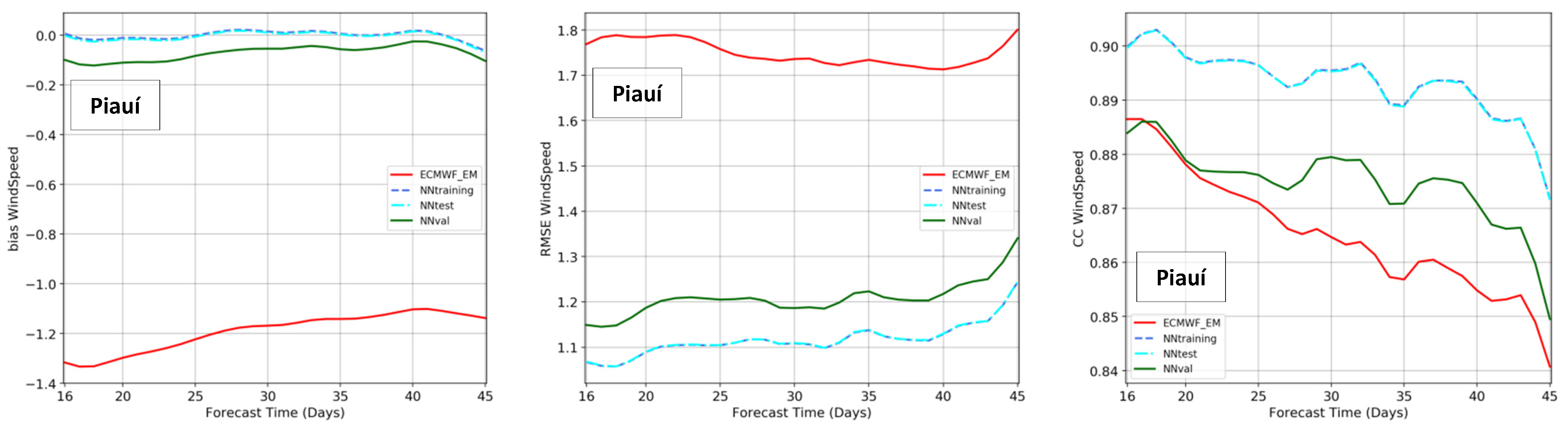
The results were assessed using the error metrics of Equations (2)–(5), applied to the training, test, and validation sets. The original ensemble mean of ECMWF was also evaluated for the same dataset, in order to provide a direct comparison of forecasts before and after the post-processing using the NN models constructed. The analyses integrated the model performances at all the stations inside each cluster. Figure 14 presents the results for short to mid-range forecasts from 1 to 15 days, and Figure 15 for long-range forecasts from 16 to 46 days. Plots are shown with bias in the left plots, where results close to zero are the most accurate; RMSE is at the center, where lower values are better; CC is in the right plots, where values close to one are those with the best predictions.
Initially, it can be seen the success of the NN models in removing bias. In both states and forecast ranges, the NNs have very small bias, between −0.1 and 0.1 m/s. The difference of NN results to the original ECMWF ensemble mean is impressive, especially in Piauí—the state where ECMWF has the largest underestimation, around 1.3 m/s. The RMSE that usually starts with low values in the nowcast and naturally grows towards the longer leads (Figure 14) also highlights the improved performance of the NN simulations. In Maranhão, the RMSE from 1.3 to 1.6 m/s was reduced to 0.9 to 1.4 m/s, a 10 to 30% improvement. In Piauí, the RMSE values from 1.7 to 1.9 m/s were reduced to 0.9 to 1.3 m/s, a more significant improvement of 30 to 50%.
Figure 14 also shows the expected decay of correlations with time, and the NNs once again enhanced the predictability when compared to the original ECMWF ensemble forecast, especially in the state of Maranhão. For this cluster, the CC from 0.89 to 0.80 was raised to 0.94 to 0.85. In the state of Piauí, Figure 14 shows a smaller improvement in correlation coefficient, indicating the difficulty of gaining performance in this cluster. Nonetheless, there is no lead time or error metrics where the NN modeling does not present better results than the original ECMWF forecast.
The analysis at longer forecast ranges is considerably different than at short and mid ranges. Lorenz [52] and Kalnay [42] explain in detail the chaotic process of the atmosphere and the accumulation and propagation of prediction errors towards forecasting days, which is clear in the first two weeks. Beyond this horizon, Robertson et al. [59] discuss the challenges of subseasonal forecasts with large uncertainties. Thus, from 16 to 46 days, the forecast errors are already high and reasonably similar in magnitude. Figure 15 confirms this pattern, where the RMSE and CC have small variations in the forecast range. The NNs, once again, are very effective in removing the systematic error, with resulting bias close to zero in both clusters. The RMSE of ECMWF in Maranhão, around 1.5 m/s, was reduced to 1.3 m/s in the NN validation set and 1.2 m/s in the NN test set. In the state of Piauí, the large RMSE between 1.7 and 1.8 m/s was reduced to 1.2 m/s in the NN validation set and 1.1 m/s in the NN test set—a better improvement than in Maranhão. The CC, in contrast, presents a more significant increase in Maranhão than in Piauí, especially the NN test set.
Joining the analyses from Figure 14 and Figure 15, it is possible to confirm that the ensembles of NNs were able to nearly remove the bias and sustain this accuracy throughout the whole forecast range, from 1 to 46 days. Similarly, the NN modeling could reduce the RMSE to values around 1 m/s, and below 1.4 m/s for all the forecast leads in both states. There were no drawbacks or cost associated with the NN implementation when compared to the original ECMWF ensemble, which was confirmed across all the metrics, months of the year, forecast times, and clusters.
6. Final Discussion
Results of Figure 13, Figure 14 and Figure 15 summarize a NN forecast product developed through multiple steps, including the initial quality control and clustering of stations, construction of a dataset for training, dimensional analysis, development of a proper NN architecture and training strategy, and development of an ensemble of NNs. In fact, the final forecast consisted of a hybrid product (Figure 8 and Equation (8)), joining the NWP from ECMWF and the post-processing NN model. This part is important to be emphasized because the large-scale and mid-to-long range atmospheric modeling is mostly performed by the global ensemble forecast of ECMWF, with the NN in charge of bias-correction and regionalization of this initial prediction. The NN model construction could preserve the simplicity of the MLP-NN, developed by Rumelhart et al. [26], with a theoretical description by Haykin [48], and environmental application at Krasnopolsky [49], which has been fundamental to the success of the tests involving the NN architecture and data structure [55], and the NN ensemble [54].
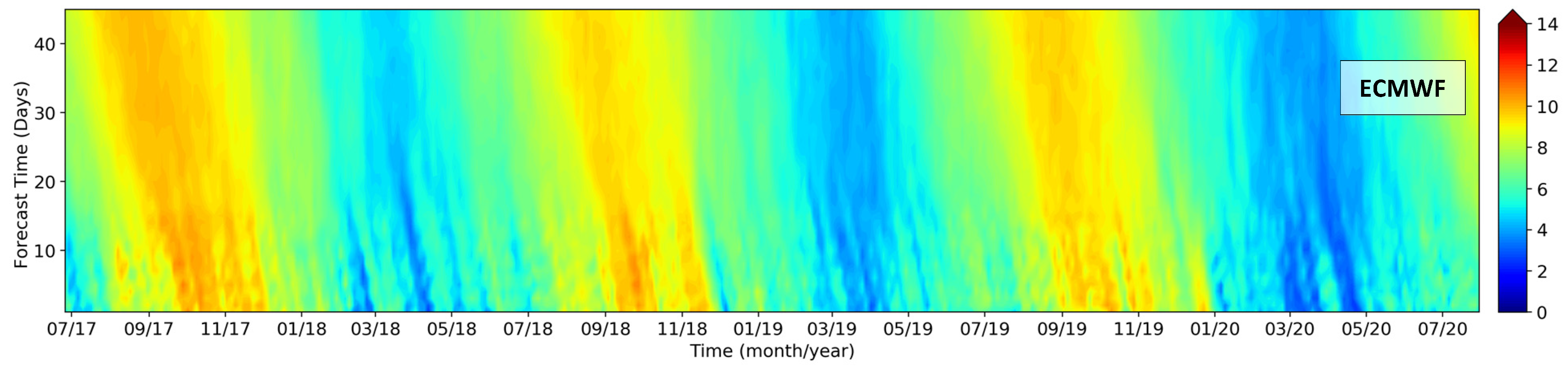
One of the most critical problems in the EMCWF prediction, discussed in this paper, is the severe underestimation of wind speeds in the state of Piauí. This problem was solved with the NN ensemble, with improved predictions for the whole forecast range from 1 to 46 days. Besides Figure 14 and Figure 15 showing the bias, Figure 16 presents a real-case simulation (reforecast) for a station in the state of Piauí, comparing the initial ECMWF forecast with the results from the post-processing NN. The underestimated ECMWF winds between August to December are visualized with yellow colors in the Figure (winds around 9 m/s), while the bias-corrected winds from the NNs are seen with orange colors (winds around 11 m/s). As a non-linear mapper, the NNs do not uplift the wind events equally or with constant rate, so the model captures the local weather patterns in the given environmental input variables, to properly bias-correct the ECMWF forecast when necessary.
The success of the NN post-processing model goes beyond the bias correction, as pointed out by Figure 14 and Figure 15. The RMSE could be reduced and CC increased, with the performance of test and validation sets ensuring the good generalization and robustness of the NN ensemble. The state of Maranhão had the best increase of CC while the state of Piauí had the best RMSE decrease—which reflects the small differences in the local climate in both states. The state of Piauí has less influence of the coastal orientation, orography, and consequently, the regional effects—having a more direct response to large-scale meteorological events, modeled by the global ECMWF ensemble. Such a prediction, as presented, has systematic errors that could be properly corrected by the NN model; however, the oscillation patterns, which influence the correlation coefficient, are mostly affected by these large-scale global phenomena as well, and so the NN as a local model could not map this part of the signal. A larger space-time machine learning model, covering a broad domain, could potentially capture this part of the forecast in Piauí. In Maranhão, however, the regional influence is more pronounced, so the CC could be better improved by the NN model; the bias, however, is not as high as in Piauí, so the contribution from the NN is relatively low. Since RMSE is a composition of scatter and systematic errors [60], the percentage of decrease of RMSE in Maranhão is also lower than the same in Piauí. Nevertheless, the NN results in Maranhão for the 15-day forecast have the same RMSE as the ECMWF forecast for 8 days, i.e., the NN post-processing represents a gain of one week in predictability.
Considering the absolute differences of error metrics between the NN results and ECMWF forecasts, the mostly improved forecast would be the longer range from 16 to 46 days. Nevertheless, even using the hybrid modeling proposed in this paper, this range remains a great challenge. This can be visualized through the differences between the NN test set and validation set. While in the range of 1–15 days, both sets have very similar values; the results completely change for the 16–46 days range, where the test set shows better values than the validation set. Such a difference suggests that the NN lacks generalization in the long-range when compared to the short-range forecast. This feature is more pronounced in the CC and RMSE, and not in the bias plots, so the NN model remains a good bias-correction tool with proper generalization even in the long-range. The impact seen in the CC and RMSE for long ranges reflects the general lack of predictability and accumulated chaos in the atmosphere that has been a meteorological challenge, especially in tropical regions.
Although a direct comparison of forecasting performances with previous studies is not possible, due to different locations and forecast ranges, it is still important to contextualize our results and method with other references and algorithms. For the short-range segment shown in Figure 14, the RMSE in the present study varied from 0.8 to 1.0 m/s and bias was between −0.1 and 0.1 m/s. The wind forecast obtained directly using the numerical model WRF described in [10] resulted in an RMSE between 1.5 and 2.1 m/s within the 48 h range. Using wavelet decomposition and recurrent neural network, [12] we obtained an RMSE from 0.76 to 2.03 m/s. At very short-term forecasts using 10 and 5 min wind sample intervals, [13] this produced an RMSE from 0.03 to 0.76 m/s, with the best performance obtained with wavelet transformation of MLP models using two training algorithms, Levenberg–Marquardt and Bayesian Regularization. Authors in [14] have shown RMSE values from 0.07 to 1.56 m/s with the best results from a new hybrid decomposition technique (HDT) combined with an ensemble empirical mode decomposition adaptive noise (CEEMDAN) and empirical wavelet transform (EWT). Authors in [15] have reached RMSE values from 0.52 to 0.89 m/s and the best performance with a wavelet analysis technique combined with negative correlation learning neural network and an ensemble structure optimized using particle-swarm optimization WAT-NCL-PSO. Authors in [16] obtained RMSE from 0.33 to 1.15 m/s using an NN model integrated with a modified firefly algorithm and particle swarm optimization. Authors in [17] obtained RMSE from 0.014 to 1.32 m/s and reported the best results using a wavelet packet decomposition, density-based spatial clustering of applications with noise, and the Elman neural network (WPD-DBSCAN-ENN), and [18] obtained RMSE from 0.26 to 0.89 m/s with the best results using singular spectrum analysis and general regression neural network with CG-BA (SSA-CG-BA-GRNN), where CG-BA is a modified bat algorithm (BA) with the conjugate gradient (CG) method developed to optimize the initial weights. These studies suggest that there is a wide range of algorithms with great potential to further improve our wind forecast, moving to more complex models and signal decomposition. Furthermore, instead of searching for one single method, [20] successfully combined a data preprocessing technique with a linear combination of multiple prediction models to produce their forecast—which is a promising multi-model ensemble approach to be implemented in the next steps of this present study.
7. Conclusions
This paper has investigated the development of a neural network (NN) post-processing model attached to a traditional global forecast (ECMWF) for bias-correction and regionalization of wind speed forecasts (daily means) with range from 1 to 46 days. The hybrid model uses a methodology where NNs simulate the residual signal that is added to the ECMWF forecast to compose a final wind prediction. The development of a 20-member ensemble of MLP-NNs, for two clusters (Maranhão and Piauí), and two forecast slices (1–15 days and 16–46 days), proved to be very efficient in reducing the bias in both states while covering the whole forecast range—where the analysis of training, test, and validation sets confirmed the proper generalization and robustness of the model. The dimension and architecture of the NN consist of a strategic part of the work, which was balanced with the computational cost, and allowed the construction of an ensemble of NNs without compromising the feasibility of its operational implementation. In this sense, there are two key achievements of the hybrid model developed: (1) first is the ability of providing very accurate local forecasts with great generalization at mid-to-long forecast ranges; (2) the successful operational implementation of such a model for daily forecasts, preserving the simplicity and low computational cost, represents a good example of a Research-to-Operation framework that will benefit the northeast of Brazil and the wind energy sector. We conclude that the ensemble of MLP-NNs described in this paper is a powerful tool to improve global NWP forecasts when multi-year and high-quality local observations are available. The methodology is currently being expanded to include options of signal decomposition [61] and wavelet transform [62,63] combined with recurrent and convolutional neural network models.
Author Contributions
All authors have contributed equally to all the steps of the present work. All authors have read and agreed to the published version of the manuscript.
Funding
This research was funded by OMEGA Energia, contract number 00004264.
Institutional Review Board Statement
Not applicable.
Informed Consent Statement
Not applicable.
Data Availability Statement
The links to the datasets used are included in the manuscript.
Acknowledgments
This study was developed from January 2020 to July 2021. Acknowledgements are due to the European Centre for Medium-Range Weather Forecasts (ECMWF) and OMEGA Energia for providing the data. The authors would like to acknowledge Luan Brito and Thiago Degola, for the great scientific contribution regarding the local weather forecast and climatology in the northeast of Brazil, as well as Fábio Almeida and Andressa D’Agostini for the technical support.
Conflicts of Interest
The authors declare no conflict of interest.
References
- Global Wind Energy Council (GWEC). Global Wind Report; Global Wind Energy Council: Brussels, Belgium, 2021; Available online: https://gwec.net/global-wind-report-2021/ (accessed on 1 February 2022).
- International Renewable Energy Agency (IRENA). Renewable Capacity Statistics; IRENA: Abu Dhabi, United Arab Emirates, 2021; ISBN 978-92-9260-342-7.
- Associação Brasileira de Energia Eólica, ABEEólica. 2021. Available online: http://abeeolica.org.br/ (accessed on 1 February 2022).
- Vinhoza, A.; Schaeffer, R. Brazil’s offshore wind energy potential assessment based on a Spatial Multi-Criteria Decision Analysis. Renew. Sustain Energy Rev. 2021, 146, 111185. [Google Scholar] [CrossRef]
- Santos, J.A.F.A.; Jong, P.; Costa, C.A.; Torres, E.A. Combining wind and solar energy sources: Potential for hybrid power generation in Brazil. Util. Policy 2020, 67, 101084. [Google Scholar] [CrossRef]
- de Silva, N.F.; Rosa, L.P.; Araújo, M.R. The utilization of wind energy in the Brazilian electric sector’s expansion. Renew. Sustain. Energy Rev. 2005, 9, 289–309. [Google Scholar] [CrossRef]
- Filgueiras, A.; Silva, T.M.V. Wind energy in Brazil—present and future. Renew. Sustain. Energy Rev. 2003, 7, 439–451. [Google Scholar] [CrossRef]
- Lima, M.A.; Mendes, L.F.R.; Mothé, G.A.; Linhares, F.G.; de Castro, M.P.P.; Da Silva, M.G.; Sthel, M.S. Renewable energy in reducing greenhouse gas emissions: Reaching the goals of the Paris agreement in Brazil. Environ. Dev. 2020, 33, 100504. [Google Scholar] [CrossRef]
- de Jong, P.; Barreto, T.B.; Tanajura, C.A.; Kouloukoui, D.; Oliveira-Esquerre, K.P.; Kiperstok, A.; Torres, E.A. Estimating the impact of climate change on wind and solar energy in Brazil using a South American regional climate model. Renew. Energy 2019, 141, 390–401. [Google Scholar] [CrossRef]
- Jacondino, W.D.; Nascimento, A.L.S.; Calvetti, L.; Fisch, G.; Beneti, C.A.A.; Paz, S.R. Hourly day-ahead wind power forecasting at two wind farms in northeast Brazil using WRF model. Energy 2021, 230, 120841. [Google Scholar] [CrossRef]
- Skamarock, W.C.; Klemp, J.B.; Dudhia, J.; Gill, D.O.; Barker, D.M.; Wang, W.; Powers, J.G. A Description of the Advanced Research WRF Version 3; University Corporation for Atmospheric Research: Boulder, CO, USA, 2008. [Google Scholar] [CrossRef]
- Zucatelli, P.J.; Nascimento, E.G.S.; Santos, A.Á.B.; Arce, A.M.G.; Moreira, D.M. An investigation on deep learning and wavelet transform to nowcast wind power and wind power ramp: A case study in Brazil and Uruguay. Energy 2021, 230, 120842. [Google Scholar] [CrossRef]
- Samet, H.; Reisi, M.; Marzbani, F. Evaluation of neural network-based methodologies for wind speed forecasting. Comput. Electr. Eng. 2019, 78, 356–372. [Google Scholar] [CrossRef]
- Qu, Z.; Mao, W.; Zhang, K.; Zhang, W.; Li, Z. Multi-step wind speed forecasting based on a hybrid decomposition technique and an improved back-propagation neural network. Renew. Energy 2019, 133, 919–929. [Google Scholar] [CrossRef]
- Ma, T.; Wang, C.; Wang, J.; Cheng, J.; Chen, X. Particle-swarm optimization of ensemble neural networks with negative correlation learning for forecasting short-term wind speed of wind farms in western China. Inf. Sci. 2019, 505, 157–182. [Google Scholar] [CrossRef]
- Begam, K.M.; Deepa, S.N. Optimized nonlinear neural network architectural models for multistep wind speed forecasting. Comput. Electr. Eng. 2019, 78, 32–49. [Google Scholar] [CrossRef]
- Yu, C.; Li, Y.; Xiang, H.; Zhang, M. Data mining-assisted short-term wind speed forecasting by wavelet packet decomposition and Elman neural network. J. Wind Eng. Ind. Aerodyn. 2018, 175, 136–143. [Google Scholar] [CrossRef]
- Xiao, L.; Qian, F.; Shao, W. Multi-step wind speed forecasting based on a hybrid forecasting architecture and an improved bat algorithm. Energy Convers. Manag. 2017, 143, 410–430. [Google Scholar] [CrossRef]
- Hu, J.; Wang, J.; Xiao, L. A hybrid approach based on the Gaussian process with t-observation model for short-term wind speed forecasts. Renew. Energy 2017, 114, 670–685. [Google Scholar] [CrossRef]
- Wang, J.; Zhang, N.; Lu, H. A novel system based on neural networks with linear combination framework for wind speed forecasting. Energy Convers. Manag. 2019, 181, 425–442. [Google Scholar] [CrossRef]
- Qu, Z.; Zhang, K.; Mao, W.; Wang, J.; Liu, C.; Zhang, W. Research and application of ensemble forecasting based on a novel multi-objective optimization algorithm for wind-speed forecasting. Energy Convers. Manag. 2017, 154, 440–454. [Google Scholar] [CrossRef]
- Wang, H.-z.; Li, G.-q.; Wang, G.-b.; Peng, J.-c.; Jiang, H.; Liu, Y.-T. Deep learning based ensemble approach for probabilistic wind power forecasting. Appl. Energy 2017, 188, 56–70. [Google Scholar] [CrossRef]
- Yu, C.; Li, Y.; Zhang, M. An improved Wavelet Transform using Singular Spectrum Analysis for wind speed forecasting based on Elman Neural Network. Energy Convers. Manag. 2017, 148, 895–904. [Google Scholar] [CrossRef]
- Daniel, L.O.; Sigauke, C.; Chibaya, C.; Mbuvha, R. Short-Term Wind Speed Forecasting Using Statistical and Machine Learning Methods. Algorithms 2020, 13, 132. [Google Scholar] [CrossRef]
- Lin, W.-H.; Wang, P.; Chao, K.-M.; Lin, H.-C.; Yang, Z.-Y.; Lai, Y.-H. Wind Power Forecasting with Deep Learning Networks: Time-Series Forecasting. Appl. Sci. 2021, 11, 10335. [Google Scholar] [CrossRef]
- Rumelhart, D.E.; Hinton, G.E.; Williams, R.J. Parallel distributed processing: Explorations in the microstructure of cognition. In Learning Internal Representations by Error Propagation; MIT Press: Cambridge, MA, USA, 1986; Volume 1. [Google Scholar]
- Xu, W.; Ning, L.; Luo, Y. Wind Speed Forecast Based on Post-Processing of Numerical Weather Predictions Using a Gradient Boosting Decision Tree Algorithm. Atmosphere 2020, 11, 738. [Google Scholar] [CrossRef]
- Jong, P.; Dargaville, R.; Silver, J.; Utembe, S.; Kiperstok, A.; Torresa, E.A. Forecasting high proportions of wind energy supplying the Brazilian Northeast electricity grid. Appl. Energy 2017, 195, 538–555. [Google Scholar] [CrossRef]
- Souza, N.B.P.; Nascimento, E.G.S.; Santos, A.A.B.; Moreira, D.M. Wind mapping using the mesoscale WRF model in a tropical region of Brazil. Energy 2022, 240, 122491. [Google Scholar] [CrossRef]
- Rocha, P.A.C.; Sousa, R.C.; Andrade, C.F.; Silva, M.E.V. Comparison of seven numerical methods for determining Weibull parameters for wind energy generation in the northeast region of Brazil. Appl. Energy 2012, 89, 395–400. [Google Scholar] [CrossRef]
- Madden, R.; Julian, P. Detection of a 40-50 day oscillation in the zonal wind in the tropical Pacific. J. Atmos. Sci. 1971, 28, 702–708. [Google Scholar] [CrossRef]
- Madden, R.; Julian, P. Description of global-scale circulation cells in the tropics with a 40-50 day period. J. Atmos. Sci. 1972, 29, 1109–1123. [Google Scholar] [CrossRef]
- World Meteorological Organization (WMO). Guide to Meteorological Instruments and Methods of Observation, 7th ed.; World Meteorological Organization: Geneva, The Switzerland, 2008; ISBN 978-92-63-10008-5. Available online: https://library.wmo.int/index.php?id=12407&lvl=notice_display# (accessed on 1 February 2022).
- Campos, R.M.; Krasnopolsky, V.; Alves, J.H.G.M.; Penny, S.G. Nonlinear wave ensemble averaging in the Gulf of Mexico using neural networks. J. Atmos. Ocean. Technol. 2019, 36, 113–127. [Google Scholar] [CrossRef]
- Ketchen, D.J.; Shook, C.L. The application of cluster analysis in Strategic Management Research: An analysis and critique. Strateg. Manag. J. 1996, 17, 441–458. [Google Scholar] [CrossRef]
- Souza, N.B.P.; Santos, J.V.C.; Nascimento, E.G.S.; Santos, A.A.B.; Moreira, D.M. Long-range correlations of the wind speed in a northeast region of Brazil. Energy 2022, 243, 122742. [Google Scholar] [CrossRef]
- Zhu, Y.; Zhou, X.; Li, W.; Hou, D.; Melhauser, C.; Sinsky, E.; Peña, M.; Fu, B.; Guan, H.; Kolczynski, W.; et al. Toward the Improvement of Subseasonal Prediction in the National Centers for Environmental Prediction Global Ensemble Forecast System. J. Geophys. Res. Atmos. 2018, 123, 6732–6745. [Google Scholar] [CrossRef]
- Chen, Y.; Zhang, S.; Zhang, W.; Peng, J.; Cai, Y. Multifactor spatio-temporal correlation model based on a combination of convolutional neural network and long short-term memory neural network for wind speed forecasting. Energy Convers. Manag. 2019, 185, 783–799. [Google Scholar] [CrossRef]
- Vlachas, P.R.; Pathak, J.; Hunt, B.R.; Sapsis, T.P.; Girvan, M.; Ott, E.; Koumoutsakos, P. Backpropagation algorithms and Reservoir Computing in Recurrent Neural Networks for the forecasting of complex spatiotemporal dynamics. Neural Netw. 2020, 126, 191–217. [Google Scholar] [CrossRef] [Green Version]
- Goulart, A.J.H.; Camargo, R. On data selection for training wind forecasting neural networks. Comput. Geosci. 2021, 155, 104825. [Google Scholar] [CrossRef]
- European Centre for Medium-Range Weather Forecasts (ECMWF). PART V: Ensemble Prediction System. In IFS Documentation-Cy47r3; ECMWF: Reading, UK, 2021. [Google Scholar] [CrossRef]
- Kalnay, E. Atmospheric Modeling, Data Assimilation and Predictability; Cambridge University Press: Cambridge, UK, 2003; p. 341. [Google Scholar] [CrossRef]
- Campos, R.M.; Alves, J.H.G.M.; Krasnopolsky, V.; Penny, S.G. Global assessments of the NCEP Ensemble Forecast System using altimeter data. Ocean Dyn. 2020, 70, 405–419. [Google Scholar] [CrossRef]
- Zhou, X.; Zhu, Y.; Hou, D.; Luo, Y.; Peng, J.; Wobus, R. Performance of the new NCEP Global Ensemble Forecast System in a parallel experiment. Weather Forecast. 2017, 32, 1989–2004. [Google Scholar] [CrossRef]
- European Centre for Medium-Range Weather Forecasts (ECMWF). 2021. Available online: https://www.ecmwf.int/en/forecasts/documentation-and-support/extended-range-forecasts/justification-ENS-extended (accessed on 1 February 2022).
- Lee, C.-Y.; Camargo, S.J.; Vitart, F.; Sobel, A.H.; Camp, J.; Wang, S.; Tippett, M.K.; Yang, Q. Subseasonal Predictions of Tropical Cyclone Occurrence and ACE in the S2S Dataset. Weather Forecast. 2020, 35, 921–938. [Google Scholar] [CrossRef]
- Camp, J.; Wheeler, M.C.; Hendon, H.H.; Gregory, P.A.; Marshall, A.G.; Tory, K.J.; Watkins, A.B.; MacLachlan, C.; Kuleshov, Y. Skilful multiweek tropical cyclone prediction in ACCESS-S1 and the role of the MJO. Q. J. R. Meteorol. Soc. 2018, 144, 1337–1351. [Google Scholar] [CrossRef]
- Haykin, S. Neural Networks: A Comprehensive Foundation, 2nd ed.; Prentice Hall: Hoboken, NJ, USA, 1999; p. 842. ISBN 81-7808-300-0. [Google Scholar]
- Krasnopolsky, V.M. The application of neural networks in the earth system sciences: Neural network emulations for complex multidimensional mappings. In Atmospheric and Oceanographic Sciences Library; Springer: Berlin, Germany, 2013; Volume 46, p. 189. [Google Scholar]
- Kingma, D.; Ba, J. Adam: A method for stochastic optimization. arXiv 2014, arXiv:1412.6980. [Google Scholar]
- Campos, R.M.; Krasnopolsky, V.; Alves, J.-H.; Penny, S.G. Improving NCEP’s global-scale wave ensemble averages using neural networks. Ocean Model. 2020, 149, 101617. [Google Scholar] [CrossRef]
- Lorenz, E.N. The predictability of hydrodynamic flow. Trans. N. Y. Acad. Sci. 1963, 25, 409–432. Available online: https://eapsweb.mit.edu/sites/default/files/Predictability_hydrodynamic_flow_1963.pdf (accessed on 1 February 2022). [CrossRef]
- Hosking, J.R.M.; Wallis, J.R. Regional Frequency Analysis-An Approach Based on L-Moments; Cambridge University Press: Cambridge, UK, 1997. [Google Scholar] [CrossRef]
- Krasnopolsky, V.M.; Lin, Y. A neural network nonlinear multimodel ensemble to improve precipitation forecasts over continental US. Adv. Meteorl. 2012, 2012, 649450. [Google Scholar] [CrossRef]
- Zaki, M.J.; Meira, W. Data Mining and Machine Learning: Fundamental Concepts and Algorithms; Cambridge University Press: Cambridge, UK, 2020; ISBN 978-1108473989. [Google Scholar]
- Hosking, J.R.M. L-moments: Analysis and estimation of distribution using linear combinations of Order statistics. J. R. Stat. Soc. Ser. B 1990, 52, 105–124. Available online: https://www.jstor.org/stable/2345653 (accessed on 1 February 2022). [CrossRef]
- Strobl, C.; Boulesteix, A.-L.; Zeileis, A.; Hothorn, T. Bias in random forest variable importance measures: Illustrations, sources and a solution. BMC Bioinform. 2007, 8, 452. [Google Scholar] [CrossRef] [PubMed] [Green Version]
- Gregorutti, B.; Michel, B.; Saint-Pierre, P. Correlation and variable importance in random forests. Stat. Comput. 2017, 27, 659–678. [Google Scholar] [CrossRef] [Green Version]
- Robertson, A.W.; Vitart, F.; Camargo, S.J. Subseasonal to Seasonal Prediction of Weather to Climate with Application to Tropical Cyclones. J. Geophys. Res. Atmos. 2020, 125, e2018JD029375. [Google Scholar] [CrossRef]
- Mentaschi, L.; Besio, G.; Cassola, F.; Mazzino, A. Problems in RMSE-based wave model validations. Ocean Model. 2013, 72, 53–58. [Google Scholar] [CrossRef]
- Zhang, Y.; Chen, B.; Pan, G.; Zhao, Y. A novel hybrid model based on VMD-WT and PCA-BP-RBF neural network for short-term wind speed forecasting. Energy Convers. Manag. 2019, 195, 180–197. [Google Scholar] [CrossRef]
- Wang, Y.; Han, L.; Liu, W.; Yang, S.; Gao, Y. Study on wavelet neural network based anomaly detection in ocean observing data series. Ocean Eng. 2019, 186, 106129. [Google Scholar] [CrossRef]
- Liu, H.; Mi, X.; Li, Y. Wind speed forecasting method based on deep learning strategy using empirical wavelet transform, long short term memory neural network and Elman neural network. Energy Convers. Manag. 2018, 156, 498–514. [Google Scholar] [CrossRef]
Figure 1.
Flowchart of the methodology and steps followed through the next sections.
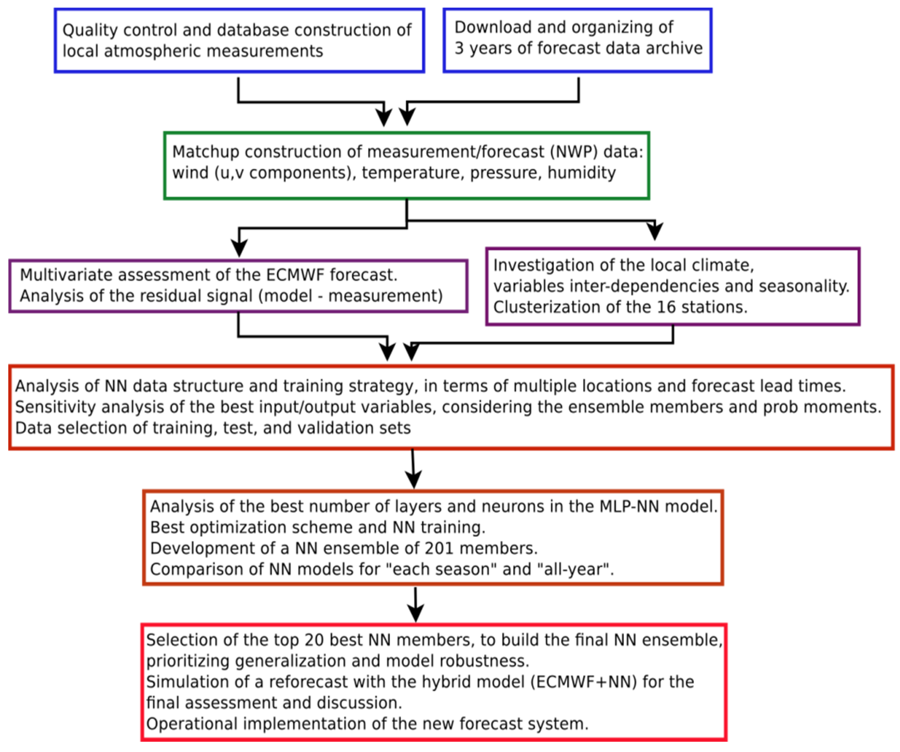
Figure 2.
Position of the atmospheric measurements located in the northeast of Brazil. The cold colors on the left indicate ten stations in the state of Maranhão, while the hot colors on the right indicate six stations in the state of Piauí. The same color standards will be used throughout this paper.

Figure 3.
Wind speed (m/s) measured by 16 anemometers located in the northeast of Brazil (Figure 2) from September 2017 to August 2020. The observations are relative to 80 m height, the default level used in this paper for both observations and forecasts.
Figure 3.
Wind speed (m/s) measured by 16 anemometers located in the northeast of Brazil (Figure 2) from September 2017 to August 2020. The observations are relative to 80 m height, the default level used in this paper for both observations and forecasts.

Figure 4.
Cluster analysis of three years of atmospheric data from 16 stations in the northeast of Brazil. (a) Elbow plot for the decision of the best number of clusters. (b) Meridional wind component versus zonal wind component, where the colors represent each station showed in Figure 2. (c) Correlation matrix (Pearson) among the 16 stations. (d) Predictive Power Score among the 16 stations.

Figure 5.
Chiclet charts of wind speed (m/s), where consecutive forecasts are plotted in the x-axis, being the forecast lead time (days) in the y-axis (panel (A)). The wind speed observations have been collocated to the exact forecast times in panel B, calculating the difference between the arithmetic ensemble mean and the measurements. Hot colors in the bottom plot (B) show overestimation of forecast winds while cold colors show underestimation. Both plots refer to station (302) at Maranhão/Brazil and the daily average is employed.


Figure 6.
ECMWF forecast error as a function of the forecast time at Maranhão, where thin lines are the ensemble members, and the solid thick lines are the arithmetic ensemble mean. Plots on the left (A,D) show the scatter error through the scatter index (SI). Center plots (B,E) show the correlation coefficient. Plots on the right (C,F) show bias (in m/s and hPa). The top plots present the wind speed errors while the bottom plots present the atmospheric pressure errors. The same color standards of Figure 2, for each station, are retained.

Figure 7.
ECMWF forecast error as a function of the forecast time at Piauí, where thin lines are the ensemble members, and the solid thick lines are the arithmetic ensemble mean. Plots on the left (A,D) show the scatter error through the scatter index (SI). Center plots (B,E) show the correlation coefficient. Plots on the right (C,F) show bias (in m/s and hPa). The top plots present the wind speed errors while the bottom plots present the atmospheric pressure errors. The same color standards of Figure 2, for each station, are retained.

Figure 8.
Schematic of the hybrid model implemented. The ECMWF ensemble forecast (green) provides the arithmetic ensemble mean of the members that is added to the NN forecast (red, the residue). If the observations had no uncertainties and errors, one could describe that the NN predicts the error of the ECMWF ensemble forecast, which is added to the original prediction to compose the final forecast product, being the wind speed the final target variable.

Figure 9.
Correlation results of four probabilistic moments (calculated using 51 ECMWF ensemble members) with the target variable of the NN model (residue of wind speed; in black). The first six bars on the left of the plot (blue and black) are related to NN outputs while the remaining bars are related to NN inputs.

Figure 10.
Illustration of the cross validation with three cycles (A) where the training set (green, blue, and black) and test set (red) are created. The bottom plot (B) presents the data split of one year of validation set (red) from the training + test set (green, blue, and black), also with three cycles.


Figure 11.
Analysis of the error as a function of the number of neurons at the intermediate layer. Despite the curve indicating the best number equal to 20, the differences among tests are small, as shown in the y-axis of the plots.
Figure 11.
Analysis of the error as a function of the number of neurons at the intermediate layer. Despite the curve indicating the best number equal to 20, the differences among tests are small, as shown in the y-axis of the plots.
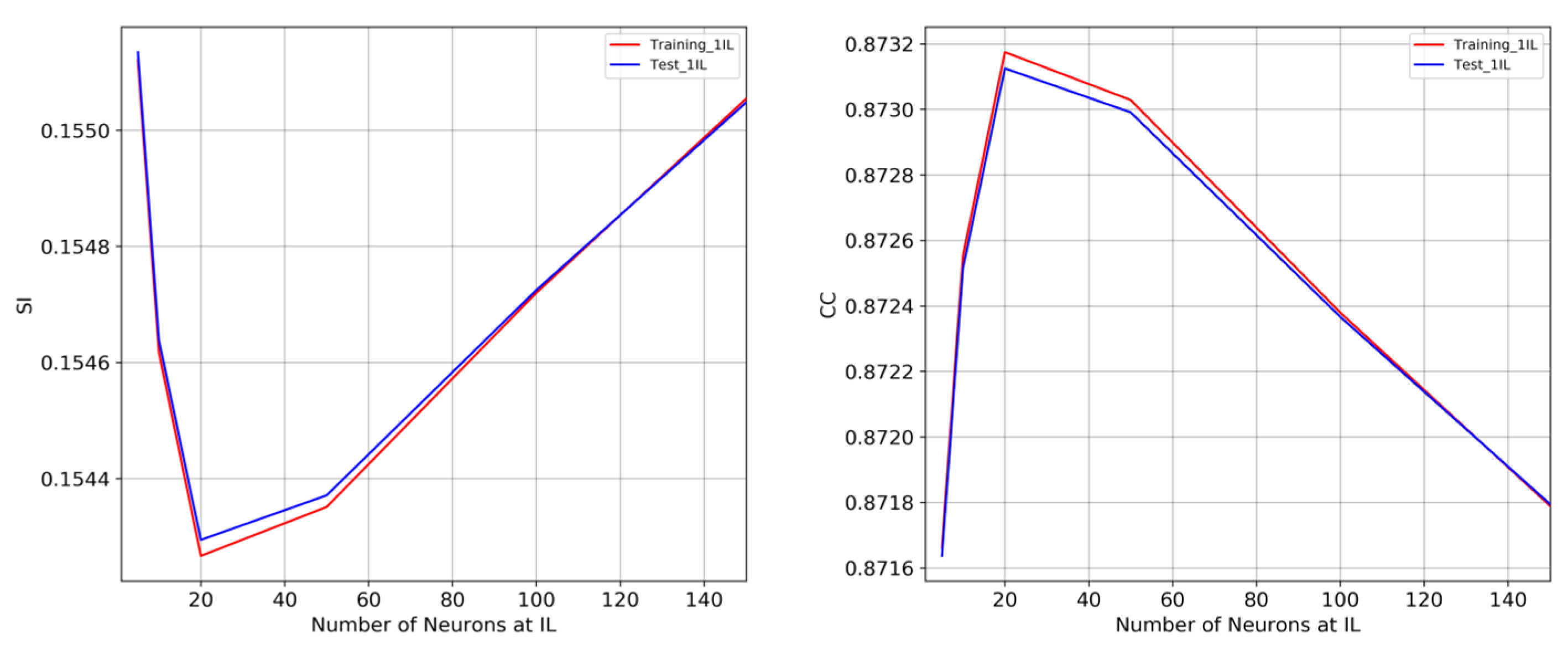
Figure 12.
Scatter plots of NN simulations of wind speed (m/s) versus observations, comparing different numbers of neurons, in the training set (left) and validation set (right). The top-left box of each plot shows the number of neurons at one or two layers.
Figure 12.
Scatter plots of NN simulations of wind speed (m/s) versus observations, comparing different numbers of neurons, in the training set (left) and validation set (right). The top-left box of each plot shows the number of neurons at one or two layers.

Figure 13.
Wind speed (m/s) Bias (top) and RMSE (bottom) of the ensemble of NNs calculated for each month of the year (x-axis). NN_AY is the all-year approach (blue); NN_SWind refers to NNs trained during the strong wind season; NN_LWind refers to NNs trained during the light wind season; EM is the ECMWF ensemble mean (red) used as reference.

Figure 14.
Assessment results of the ensemble of NNs when compared to the initial ECMWF forecast, for the forecast range from 1 to 15 days. Wind speed (m/s) Bias (lest), RMSE (center), and correlation coefficient (CC; right) are presented. Colors refer to: NN training set in dashed blue, NN test set in dashed-dotted cyan; NN validation set in green; the ECMWF forecast in red.

Figure 15.
Assessment results of the ensemble of NNs when compared to the initial ECMWF forecast, for the forecast range from 16 to 46 days. Wind speed (m/s) Bias (lest), RMSE (center), and correlation coefficient (CC; right) are presented. Colors refer to: NN training set in dashed blue, NN test set in dashed-dotted cyan; NN validation set in green; the ECMWF forecast in red.


Figure 16.
Chiclet chart presenting the reforecast results of wind speed (m/s) for the state of Piauí.
Figure 16.
Chiclet chart presenting the reforecast results of wind speed (m/s) for the state of Piauí.


Publisher’s Note: MDPI stays neutral with regard to jurisdictional claims in published maps and institutional affiliations. |
© 2022 by the authors. Licensee MDPI, Basel, Switzerland. This article is an open access article distributed under the terms and conditions of the Creative Commons Attribution (CC BY) license (https://creativecommons.org/licenses/by/4.0/).
Share and Cite
MDPI and ACS Style
Campos, R.M.; Palmeira, R.M.J.; Pereira, H.P.P.; Azevedo, L.C. Mid-to-Long Range Wind Forecast in Brazil Using Numerical Modeling and Neural Networks. Wind 2022, 2, 221-245. https://doi.org/10.3390/wind2020013
AMA Style
Campos RM, Palmeira RMJ, Pereira HPP, Azevedo LC. Mid-to-Long Range Wind Forecast in Brazil Using Numerical Modeling and Neural Networks. Wind. 2022; 2(2):221-245. https://doi.org/10.3390/wind2020013
Chicago/Turabian StyleCampos, Ricardo M., Ronaldo M. J. Palmeira, Henrique P. P. Pereira, and Laura C. Azevedo. 2022. "Mid-to-Long Range Wind Forecast in Brazil Using Numerical Modeling and Neural Networks" Wind 2, no. 2: 221-245. https://doi.org/10.3390/wind2020013