
An Inverse Method for Wind Turbine Blade Design with Given Distributions of Load Coefficients


Abstract
:1. Introduction
2. The Inverse Method for Blade Design
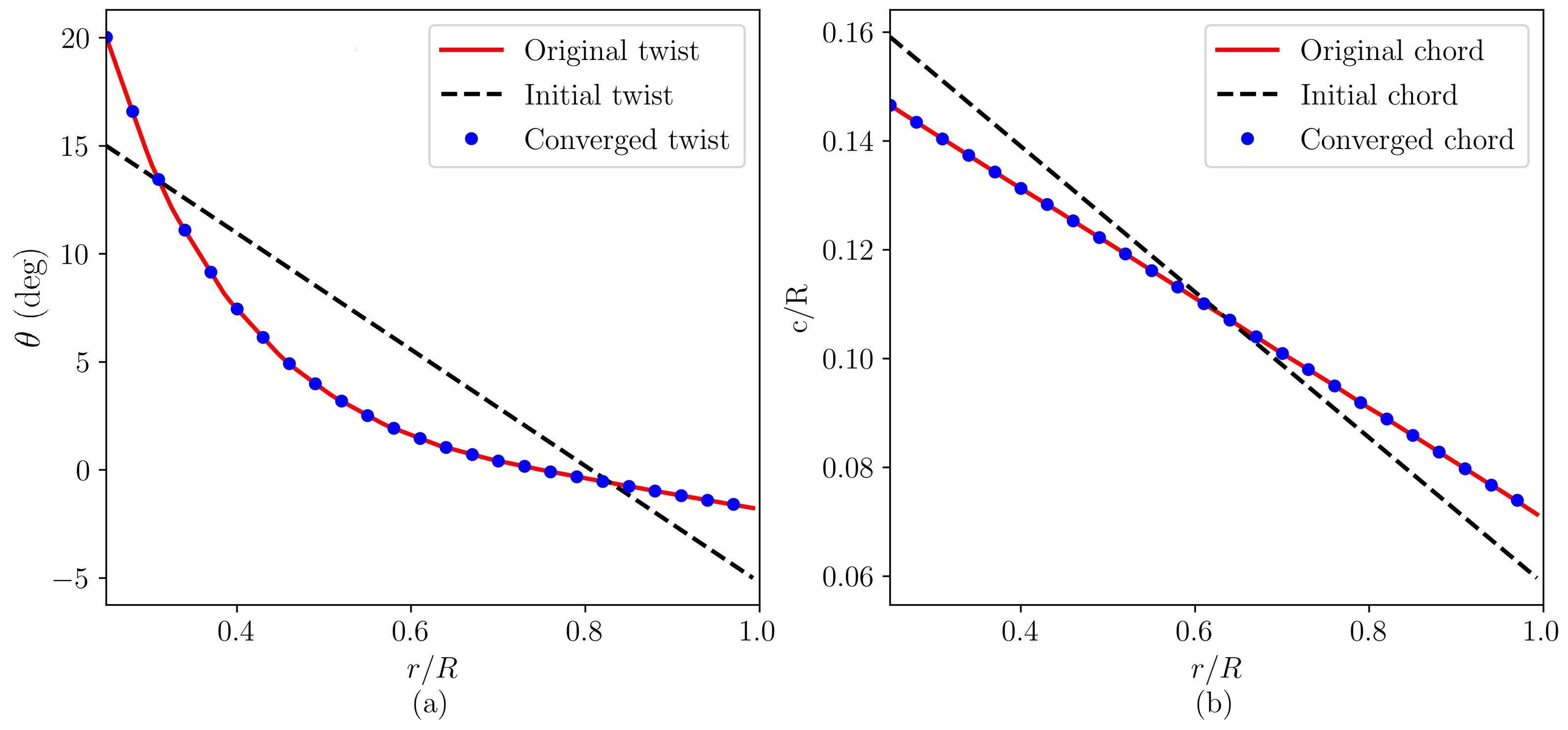
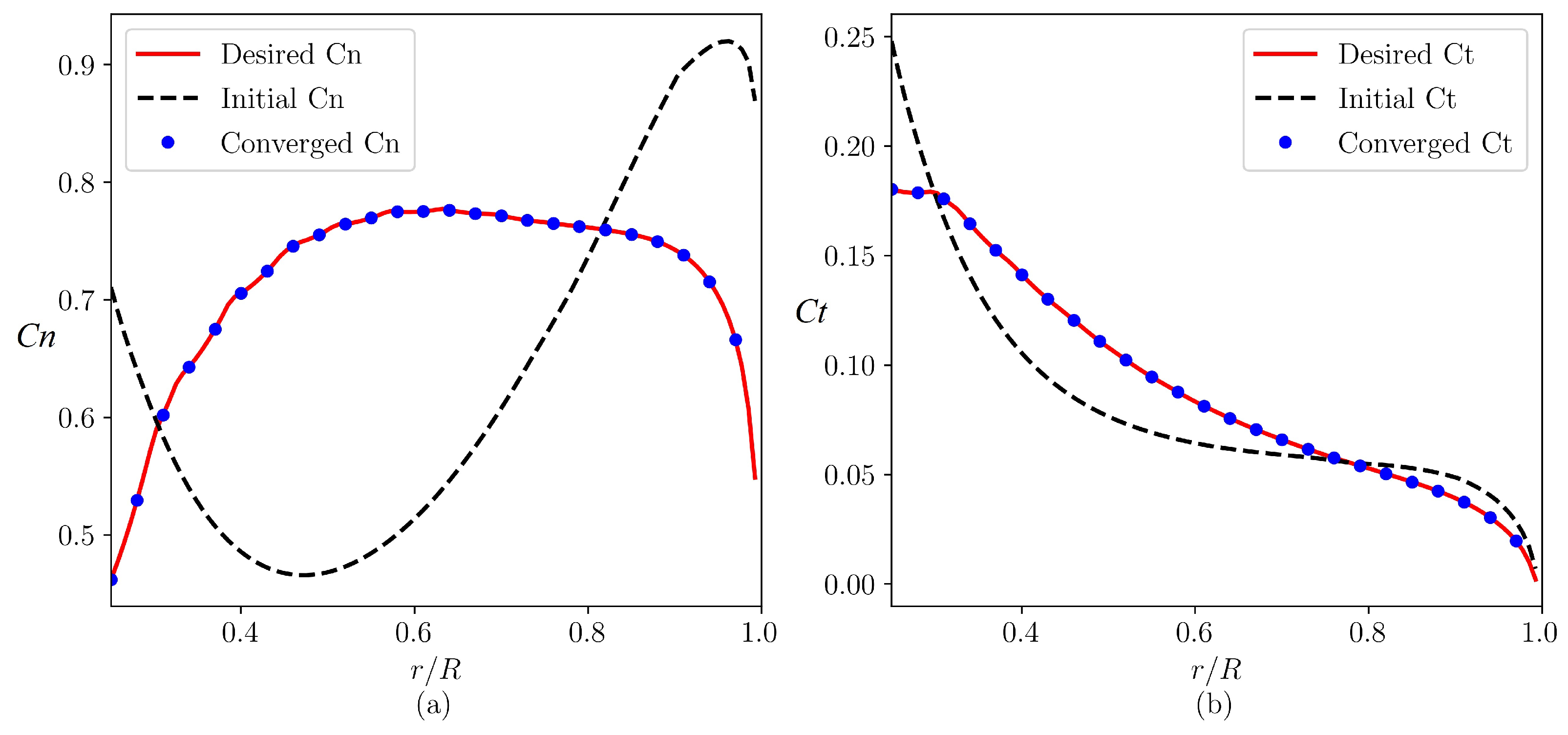
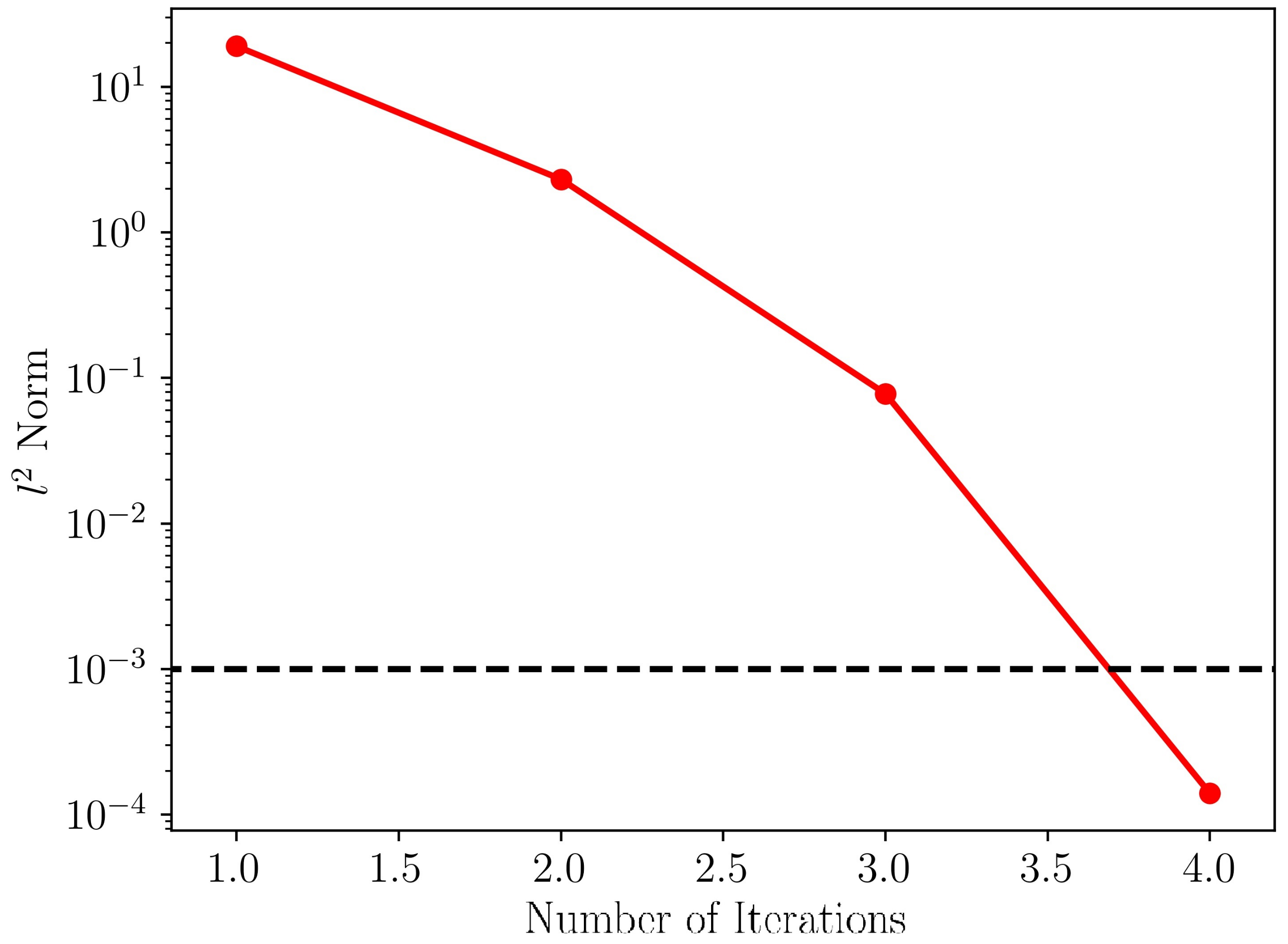
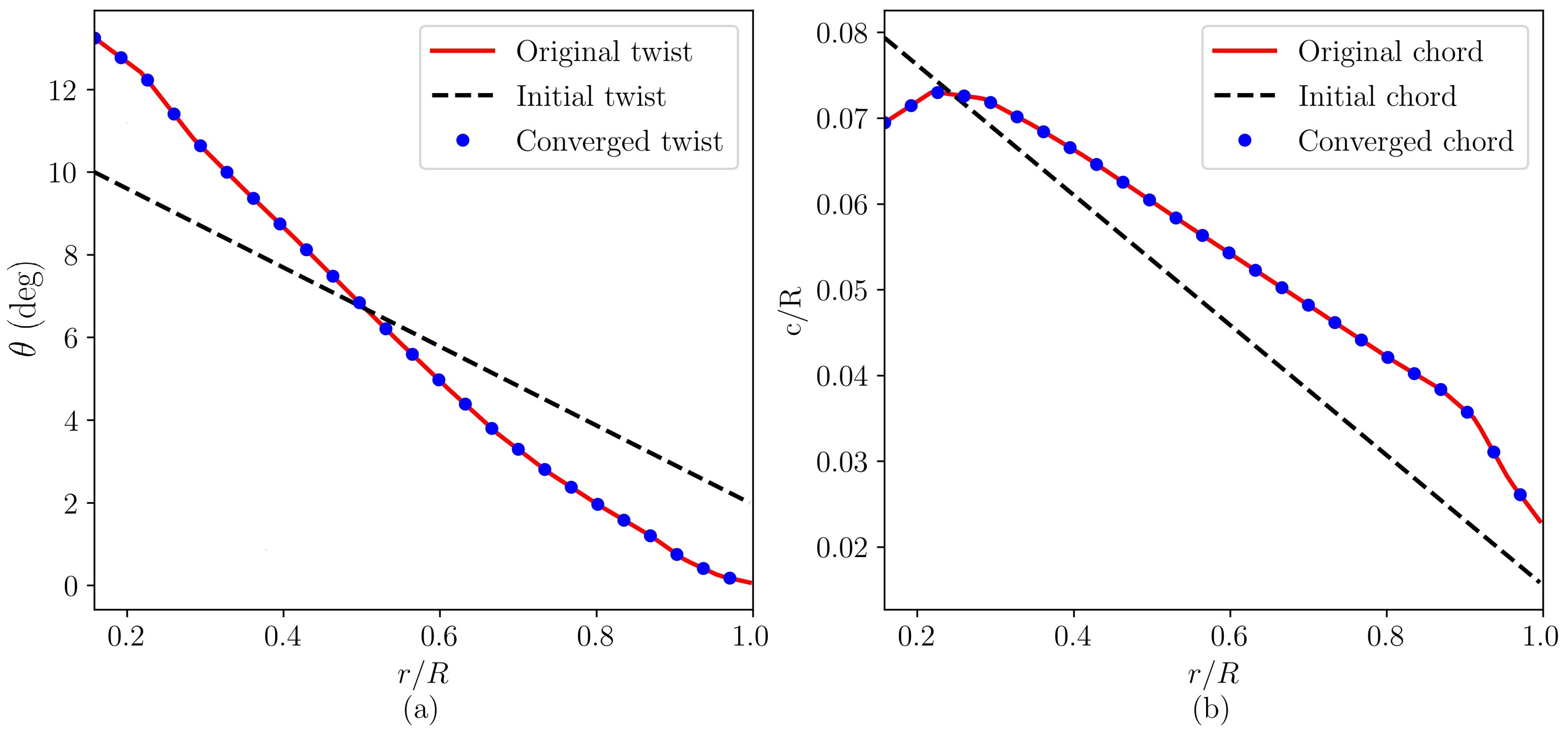
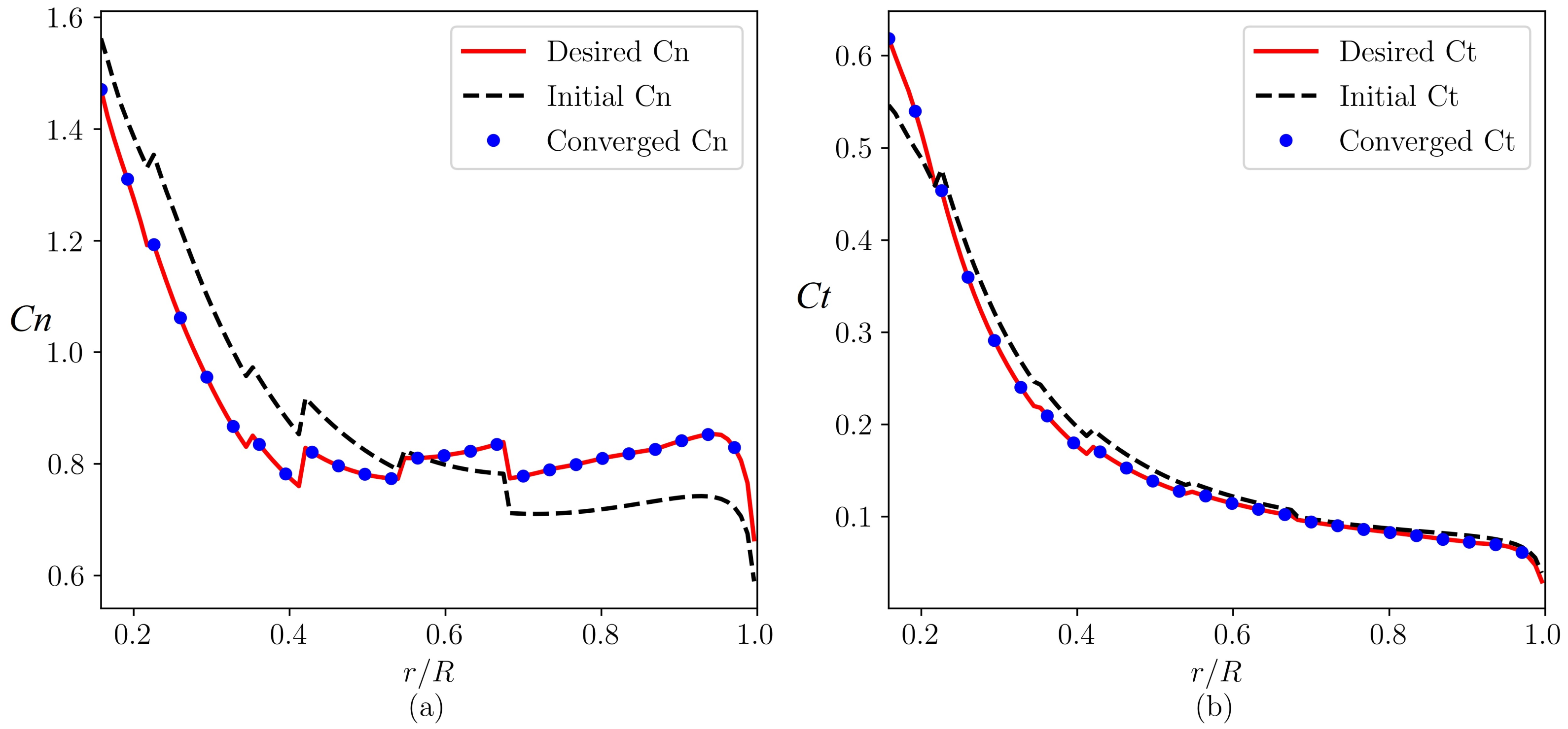
3. Validations
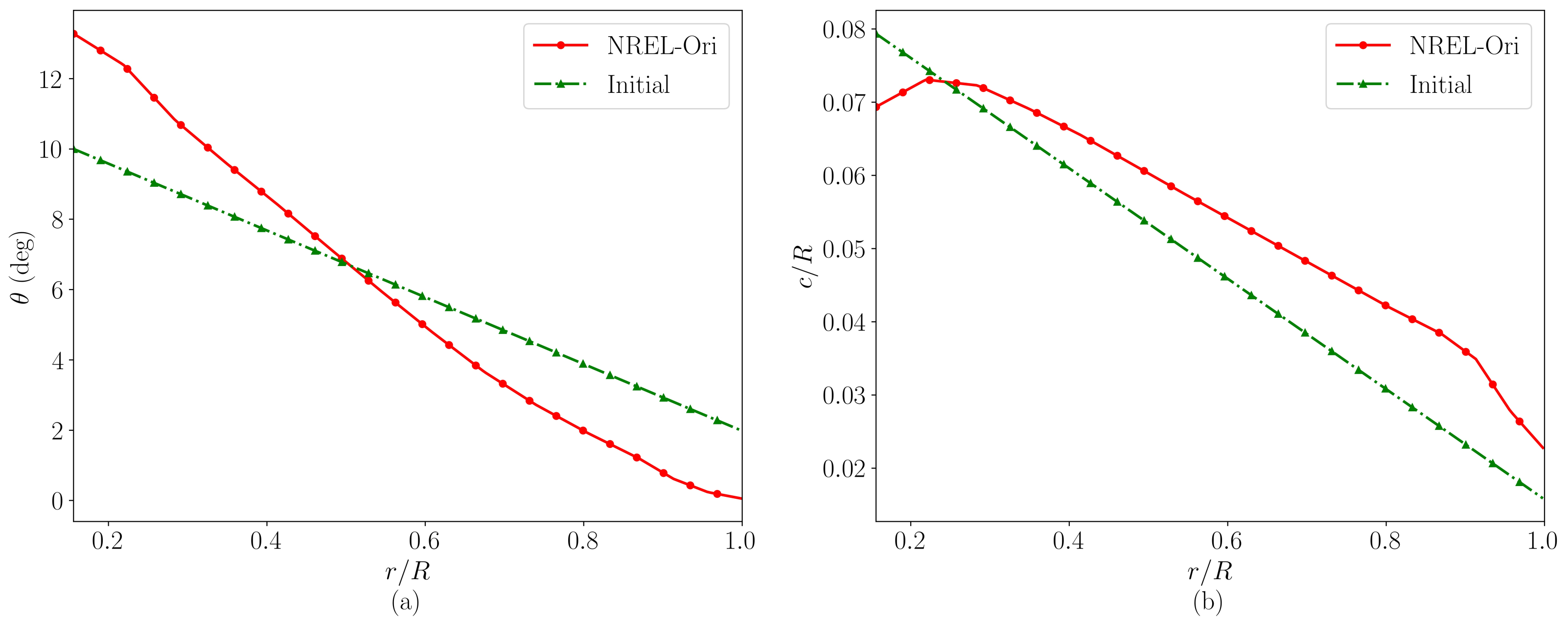
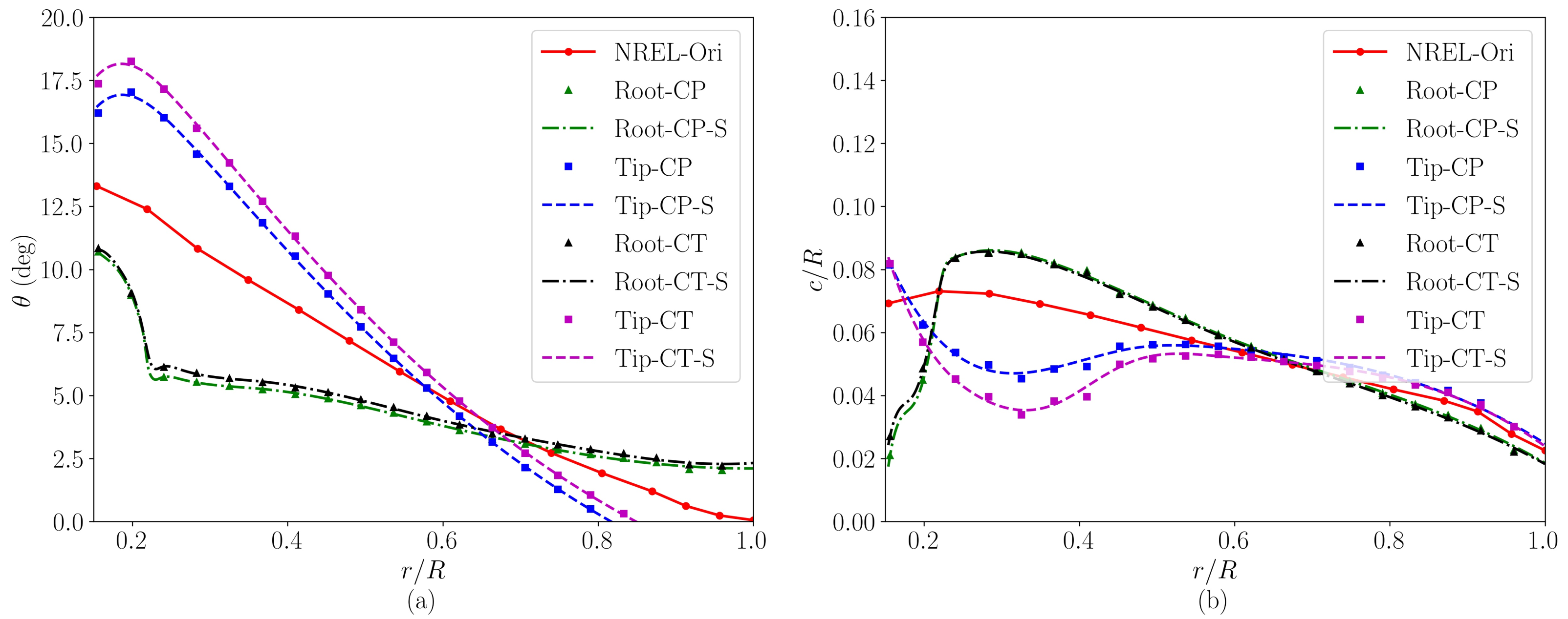
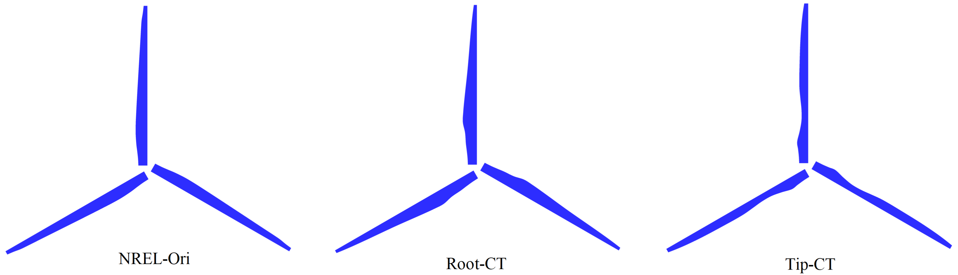
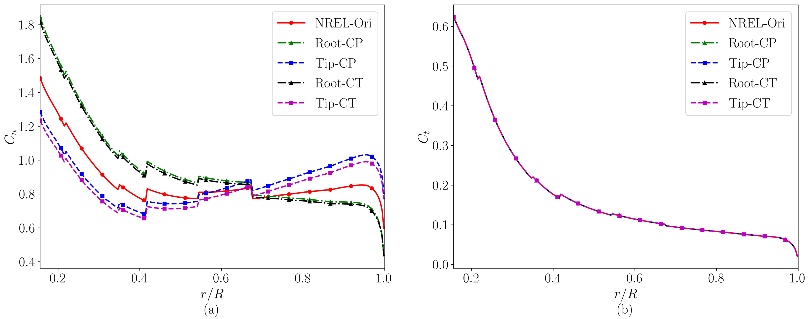
4. Four Variants of the NREL 5 MW Wind Turbine
5. Conclusions
Author Contributions
Funding
Institutional Review Board Statement
Informed Consent Statement
Data Availability Statement
Conflicts of Interest
Appendix A. Implementation of the Blade-Element Momentum Method
- (1)
- Initialize the axial induction factor (a) and the tangential induction factor ():
- (2)
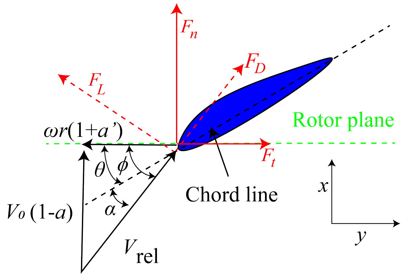
- Calculate the local inflow angle , which is the angle between relative incoming velocity and the rotor plane as shown in Figure A2, and computed via:where is the relative incoming velocity experienced by the turbine blades defined as a combination of the hindered inflow velocity (), and the induced velocity of the blades () due to the interaction between the blades and the surrounding fluids, in which is the angular velocity of the turbine. is the free incoming wind speed.
- (3)
- Calculate the local angle of attack (), which is the angle between the relative incoming velocity and the chord line as shown in Figure A2.where is the local pitch angle.
- (4)
- Read the lift coefficient () and the drag coefficient () from corresponding tables, which can be obtained from experiments or simulations (e.g., XFOIL [35]). The lift and drag can be calculated as follows:where c is the chord length, and is the air density. and (as shown in red dashed lines in Figure A2) are the lift and drag forces that are perpendicular to and are aligned with the direction of , respectively.
- (5)
- Calculate the local normal and tangential force coefficients ( and ) as follows:where and are the normal force and tangential force computed as follows:
- (6)
- Calculate a and by using the Glauert correction for the high axial induction factor a high and Prandtl’s tip correction [39] using the following expression,Here, is the Prandtl’s tip correction meanwhile is the solidity, which are in the following form,where R is the radial of the blade, and B denotes the number of blades. In the expressions for the induction factors, X and K are computed via:
- (7)
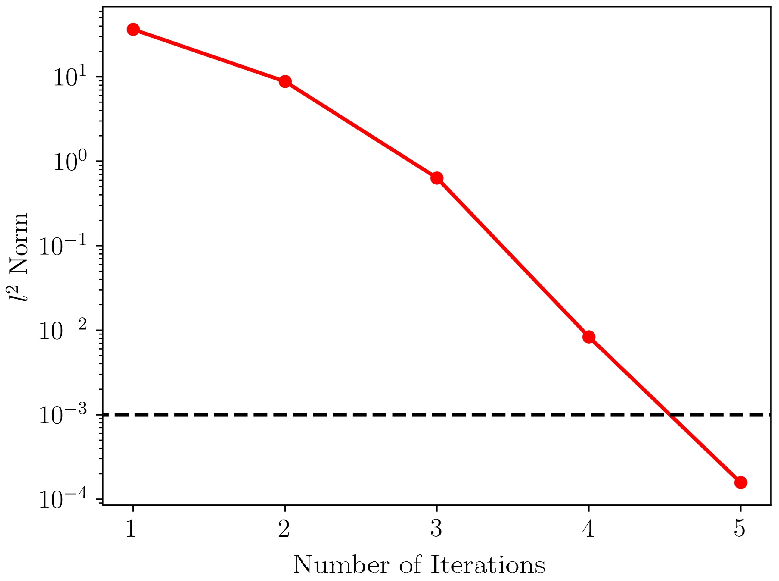
- If the differences in the magnitudes of a and are higher than a threshold, go to Step 2, else finish the loop and go to Step 8.
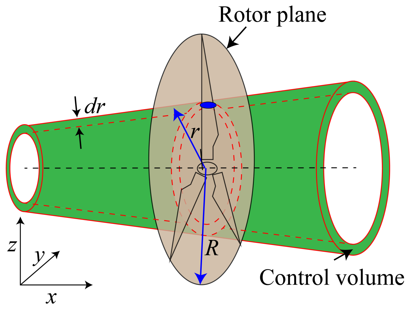
- (8)
- After obtaining the converged induction factors a and , the loads including the normal force () and the tangential force () at each radial positions are used to calculate the thrust () and torque () on the control volume of thickness as follows:At the end, integrating over the whole blades to obtain the thrust T, the power , and the corresponding thrust coefficient and the power coefficient can be obtained as:
References
- Davis, S.J.; Lewis, N.S.; Shaner, M.; Aggarwal, S.; Arent, D.; Azevedo, I.L.; Benson, S.M.; Bradley, T.; Brouwer, J.; Chiang, Y.M.; et al. Net-zero emissions energy systems. Science 2018, 360, eaas9793. [Google Scholar] [CrossRef] [PubMed] [Green Version]
- International Energy Agency Global Energy. CO2 Status Report 2018; International Energy Agency: Paris, France, 2019. [Google Scholar]
- Li, C.; Abraham, A.; Li, B.; Hong, J. Incoming flow measurements of a utility-scale wind turbine using super-large-scale particle image velocimetry. J. Wind. Eng. Ind. Aerodyn. 2020, 197, 104074. [Google Scholar] [CrossRef]
- Antonini, E.G.; Caldeira, K. Atmospheric pressure gradients and Coriolis forces provide geophysical limits to power density of large wind farms. Appl. Energy 2021, 281, 116048. [Google Scholar] [CrossRef]
- Yang, X.; Boomsma, A.; Sotiropoulos, F.; Resor, B.R.; Maniaci, D.C.; Kelley, C.L. Effects of spanwise blade load distribution on wind turbine wake evolution. In Proceedings of the 33rd Wind Energy Symposium, Kissimmee, FL, USA, 5–9 January 2015; p. 0492. [Google Scholar]
- Allen, J.; Young, E.; Bortolotti, P.; King, R.; Barter, G. Blade planform design optimization to enhance turbine wake control. Wind Energy 2022. [Google Scholar] [CrossRef]
- Tangler, J.; Kocurek, D. Wind turbine post-stall airfoil performance characteristics guidelines for blade-element momentum methods. In Proceedings of the 43rd AIAA Aerospace Sciences Meeting and Exhibit, Reno, NV, USA, 10–13 January 2005; p. 591. [Google Scholar]
- Madsen, H.A.; Bak, C.; Døssing, M.; Mikkelsen, R.; Øye, S. Validation and modification of the Blade Element Momentum theory based on comparisons with actuator disc simulations. Wind Energy 2010, 13, 373–389. [Google Scholar] [CrossRef]
- Hansen, M.O. Aerodynamics of Wind Turbines; Routledge: London, UK, 2015. [Google Scholar]
- Mahmuddin, F. Rotor blade performance analysis with blade element momentum theory. Energy Procedia 2017, 105, 1123–1129. [Google Scholar] [CrossRef]
- Chattot, J.J. Optimization of wind turbines using helicoidal vortex model. J. Sol. Energy Eng. 2003, 125, 418–424. [Google Scholar] [CrossRef]
- Hallissy, J.; Chattot, J.J. Validation of helicoidal vortex model with the NREL unsteady aerodynamic experiment. In Proceedings of the 43rd AIAA Aerospace Sciences Meeting and Exhibit, Reno, NV, USA, 10–13 January 2005; p. 1454. [Google Scholar]
- Chattot, J.J. Helicoidal vortex model for steady and unsteady flows. Comput. Fluids 2006, 35, 733–741. [Google Scholar] [CrossRef]
- Chattot, J.J. Effects of blade tip modifications on wind turbine performance using vortex model. Comput. Fluids 2009, 38, 1405–1410. [Google Scholar] [CrossRef]
- Yang, X.; Kang, S.; Sotiropoulos, F. Computational study and modeling of turbine spacing effects in infinite aligned wind farms. Phys. Fluids 2012, 24, 115107. [Google Scholar] [CrossRef]
- Yang, D.; Meneveau, C.; Shen, L. Large-eddy simulation of offshore wind farm. Phys. Fluids 2014, 26, 025101. [Google Scholar] [CrossRef]
- Yang, X.; Sotiropoulos, F.; Conzemius, R.J.; Wachtler, J.N.; Strong, M.B. Large-eddy simulation of turbulent flow past wind turbines/farms: the Virtual Wind Simulator (VWiS). Wind Energy 2015, 18, 2025–2045. [Google Scholar] [CrossRef]
- Stevens, R.J.; Meneveau, C. Flow structure and turbulence in wind farms. Annu. Rev. Fluid Mech. 2017, 49, 311–339. [Google Scholar] [CrossRef]
- Li, Z.; Yang, X. Evaluation of Actuator Disk Model Relative to Actuator Surface Model for Predicting Utility-Scale Wind Turbine Wakes. Energies 2020, 13, 3574. [Google Scholar] [CrossRef]
- Yang, X.; Pakula, M.; Sotiropoulos, F. Large-eddy simulation of a utility-scale wind farm in complex terrain. Appl. Energy 2018, 229, 767–777. [Google Scholar] [CrossRef]
- Sotiropoulos, F.; Yang, X. Immersed boundary methods for simulating fluid–structure interaction. Prog. Aerosp. Sci. 2014, 65, 1–21. [Google Scholar] [CrossRef]
- Qin, J.; Andreopoulos, Y.; Jiang, X.; Dong, G.; Chen, Z. Efficient coupling of direct forcing immersed boundary-lattice Boltzmann method and finite element method to simulate fluid-structure interactions. Int. J. Numer. Methods Fluids 2020, 92, 545–572. [Google Scholar] [CrossRef]
- Qin, J.; Kolahdouz, E.M.; Griffith, B.E. An immersed interface-lattice Boltzmann method for fluid–structure interaction. J. Comput. Phys. 2021, 428, 109807. [Google Scholar] [CrossRef]
- Selig, M.S.; Tangler, J.L. Development and application of a multipoint inverse design method for horizontal axis wind turbines. Wind Eng. 1995, 19, 91–105. [Google Scholar]
- Tang, X.; Huang, X.; Peng, R.; Liu, X. A direct approach of design optimization for small horizontal axis wind turbine blades. Procedia CIRP 2015, 36, 12–16. [Google Scholar] [CrossRef] [Green Version]
- Schubel, P.J.; Crossley, R.J. Wind turbine blade design. Energies 2012, 5, 3425–3449. [Google Scholar] [CrossRef] [Green Version]
- Méndez, J.; Greiner, D. Wind blade chord and twist angle optimization using genetic algorithms. In Proceedings of the Fifth International Conference on Engineering Computational Technology, Las Palmas de Gran Canaria, Spain, 12–15 September 2006; pp. 12–15. [Google Scholar]
- Lee, S. Inverse design of horizontal axis wind turbine blades using a vortex line method. Wind Energy 2015, 18, 253–266. [Google Scholar] [CrossRef] [Green Version]
- Jonkman, J.; Butterfield, S.; Musial, W.; Scott, G. Definition of a 5-MW Reference Wind Turbine for Offshore System Development; Technical Report; National Renewable Energy Lab. (NREL): Golden, CO, USA, 2009. [Google Scholar]
- Siddiqui, M.S.; Rasheed, A.; Tabib, M.; Kvamsdal, T. Numerical investigation of modeling frameworks and geometric approximations on NREL 5 MW wind turbine. Renew. Energy 2019, 132, 1058–1075. [Google Scholar] [CrossRef]
- Yang, X.; Sotiropoulos, F. A new class of actuator surface models for wind turbines. Wind Energy 2018, 21, 285–302. [Google Scholar] [CrossRef] [Green Version]
- Somers, D.M. Design and Experimental Results for the S809 Airfoil; Technical Report; National Renewable Energy Lab.: Golden, CO, USA, 1997. [Google Scholar]
- Giguere, P.; Selig, M.S. Design of a Tapered and Twisted Blade for the NREL Combined Experiment Rotor; Technical Report; National Renewable Energy Lab.: Golden, CO, USA, 1999. [Google Scholar]
- Hand, M.; Simms, D.; Fingersh, L.; Jager, D.; Cotrell, J.; Schreck, S.; Larwood, S. Unsteady Aerodynamics Experiment Phase VI: Wind Tunnel Test Configurations and Available Data Campaigns; Technical Report; National Renewable Energy Lab.: Golden, CO, USA, 2001. [Google Scholar]
- Drela, M. XFOIL: An analysis and design system for low Reynolds number airfoils. In Low Reynolds Number Aerodynamics; Springer: Berlin/Heidelberg, Germany, 1989; pp. 1–12. [Google Scholar]
- Chapra, S.C.; Canale, R.P. Numerical Methods for Engineers; Mcgraw-Hill: New York, NY, USA, 2011; Volume 2. [Google Scholar]
- Tahani, M.; Kavari, G.; Masdari, M.; Mirhosseini, M. Aerodynamic design of horizontal axis wind turbine with innovative local linearization of chord and twist distributions. Energy 2017, 131, 78–91. [Google Scholar] [CrossRef]
- Dong, G.; Li, Z.; Qin, J.; Yang, X. Predictive capability of actuator disk models for wakes of different wind turbine designs. Renew. Energy 2022, 188, 269–281. [Google Scholar] [CrossRef]
- Glauert, H. Airplane propellers. In Aerodynamic Theory; Springer: Berlin/Heidelberg, Germany, 1935; pp. 169–360. [Google Scholar]


| Turbines | Number of Blades | TSR | Pitch (deg) | R (m) | Rb (m) |
|---|---|---|---|---|---|
| NREL S809 | 2 | 8 | 0 | 5.029 | 1.51 |
| NREL 5 MW | 3 | 8 | 0 | 63.0 | 9.7 |
| Constraints | Turbines | Differences | Differences | ||
|---|---|---|---|---|---|
| Same | NREL-Ori | 0.770 | 0.506 | - | - |
| Root-CP | 0.791 | 0.506 | +2.76% | - | |
| Tip-CP | 0.835 | 0.506 | +8.47% | - | |
| Same | Root-CT | 0.770 | 0.50 | - | −1.33% |
| Tip-CT | 0.770 | 0.483 | - | −4.68% |
| Constraints | Turbines | Differences | |
|---|---|---|---|
| Same | NREL-Ori | 0.525 | - |
| Root-CP | 0.508 | −3.24% | |
| Tip-CP | 0.604 | 15.1% | |
| Same | Root-CT | 0.491 | −6.48% |
| Tip-CT | 0.563 | 7.24% |
Publisher’s Note: MDPI stays neutral with regard to jurisdictional claims in published maps and institutional affiliations. |
© 2022 by the authors. Licensee MDPI, Basel, Switzerland. This article is an open access article distributed under the terms and conditions of the Creative Commons Attribution (CC BY) license (https://creativecommons.org/licenses/by/4.0/).
Share and Cite
Dong, G.; Qin, J.; Li, Z.; Yang, X. An Inverse Method for Wind Turbine Blade Design with Given Distributions of Load Coefficients. Wind 2022, 2, 175-191. https://doi.org/10.3390/wind2010010
Dong G, Qin J, Li Z, Yang X. An Inverse Method for Wind Turbine Blade Design with Given Distributions of Load Coefficients. Wind. 2022; 2(1):175-191. https://doi.org/10.3390/wind2010010
Chicago/Turabian StyleDong, Guodan, Jianhua Qin, Zhaobin Li, and Xiaolei Yang. 2022. "An Inverse Method for Wind Turbine Blade Design with Given Distributions of Load Coefficients" Wind 2, no. 1: 175-191. https://doi.org/10.3390/wind2010010
APA StyleDong, G., Qin, J., Li, Z., & Yang, X. (2022). An Inverse Method for Wind Turbine Blade Design with Given Distributions of Load Coefficients. Wind, 2(1), 175-191. https://doi.org/10.3390/wind2010010