Proceeding Paper

Geodesic Least Squares: Robust Regression Using Information Geometry †

by
Geert Verdoolaege
Department of Applied Physics, Ghent University, 9000 Ghent, Belgium
Presented at the 42nd International Workshop on Bayesian Inference and Maximum Entropy Methods in Science and Engineering, Garching, Germany, 3–7 July 2023.
Phys. Sci. Forum 2023, 9(1), 5; https://doi.org/10.3390/psf2023009005
Published: 27 November 2023

Abstract

:
Geodesic least squares (GLS) is a regression technique that operates in spaces of probability distributions. Based on the minimization of the Rao geodesic distance between two probability models of the response variable, GLS is robust against outliers and model misspecification. The method is very simple, without any tuning parameters, owing to its solid foundations rooted in information geometry. Here, we illustrate the robustness properties of GLS using applications in the fields of magnetic confinement fusion and astrophysics. Additional interpretation is gained from visualizations using several models for the manifold of Gaussian probability distributions.

1. Introduction

Geodesic least squares is a relatively new technique for regression analysis in a regular Euclidean data space, which takes into account uncertainty estimates (error bars) on all regression variables [1]. It is a minimum distance technique that uses the geodesic distance (Rao distance) on a statistical manifold, as studied in the field of information geometry [2,3]. Crucially, the method is easily implemented, yet it exhibits good robustness properties in the presence of outliers and model uncertainty.
With this contribution, on the one hand, we aim to demonstrate the robustness of the technique with recent and new applications. On the other hand, we intend to stress the considerable value, in some domains of application, of analysis techniques that are easy to implement, requiring little tuning or expert knowledge, while addressing shortcomings of overly simple data analysis techniques that are nevertheless commonly employed. Hence, we aim to promote the use of geometric methods in machine learning by showing that proper treatment of the complex, nonlinear character of certain data can greatly improve the performance of even the simplest analysis techniques. We focus on the estimation of power laws, which are ubiquitous in various domains, such as astronomy, biology and geology, reflecting scale invariance and details of the underlying dynamical processes.
Two applications are targeted in this work. The first is situated in the domain of magnetic confinement fusion (MCF), specifically the critical scaling law for the energy confinement time. MCF is a field where the methods of modern data science have only recently been introduced and where the ease of implementation and interpretation are likely to accelerate the widespread adoption of new analysis techniques. The second application concerns a key scaling law in astrophysics: the baryonic Tully–Fisher relation. This is a remarkably tight relation between the total baryonic mass of disk galaxies and their rotational velocity, which is of great practical and theoretical significance in astrophysics and cosmology.
The exposition starts with a description of the GLS regression technique in Section 2. We then move to the application in fusion science in Section 3, followed by the astrophysical application in Section 4. Section 5 concludes the paper.

2. Geodesic Least Squares Regression

GLS relies on the concept of a statistical manifold, which is a Riemannian manifold that uses the Fisher information as a metric tensor. As such, it is a nonlinear space wherein the points themselves represent probability distributions. Geodesics, i.e., curves of a locally minimal distance between points on the manifold, can be constructed using the Levi–Civita connection, from which a geodesic distance can be obtained. Given a parametric probability model p ( { x m } | { θ j } ) for variables x m ( m = 1 , , M ) with parameters θ j ( j = 1 , , n par ), the Fisher information (covariance of the score) provides a unique metric tensor, with elements given by
g i j = E 2 θ i θ j ln p { x m } | { θ k } , i , j , k = 1 , , n par .
For instance, in the case of a univariate normal distribution p ( x | μ , σ ) , parametrized by its mean μ and standard deviation σ , the Fisher information matrix is [4]
I ( μ , σ ) = 1 σ 2 1 0 0 2 .
To explain the principle of GLS regression, let us assume an exact functional relationship η = f ( { ξ m } , α j ) , parametrized by the set α j ( j = 1 , , n par ), between a set of hidden predictor variables ξ 1 , …, ξ n pred and a single hidden response variable η (in the remainder of this paper, we no longer make a notational distinction between covariantly and contravariantly transforming quantities). Let us also consider additive uncertainty on all variables, yielding the respective measurable variables y, x 1 , …, x n pred :
y = η + ϵ y , x 1 = ξ 1 + ϵ x 1 ,
For simplicity, here we consider zero-mean normal error distributions, but other models can be used as well:
ϵ y N 0 , σ y , ϵ x 1 N 0 , σ x 1 ,
Importantly, it is assumed that an estimate of the measurement uncertainties is available, determined by the experimentalist. This will be used to construct a modeled distribution for the data. Furthermore, we consider the general case, which will be useful in Section 3, where the data consist of n obs , k independent observations of the response and predictor variables from a class k (e.g., a fusion device), out of a total of n class classes (e.g., multiple fusion devices). The unobserved values ξ m , i k , k ( m = 1 , , n pred , i k = 1 , , n obs , k , k = 1 , , n class ) need to be marginalized out. If f is linear,
η = α 0 + j = 1 n pred α j ξ j , ( n par = n pred + 1 )
and then the joint likelihood is again Gaussian:
p { y i k , k } , { x j , i k , k } | { α 0 , α j } = k = 1 n class i k = 1 n obs , k 1 2 π σ mod , i k , k 2 exp 1 2 y i k , k f { x j , i k , k , α 0 , α j } 2 σ mod , i k , k 2 ,
where [5]
σ mod , i k , k 2 = σ y , i k , k 2 + j = 1 n pred α j 2 σ x j , i k , k 2 ,
and the standard deviations σ x j , i k , k may in general be different for each data point. Note that, in Equation (1), we have plugged the measured data points x j , i k , k into f. The marginalization causes their uncertainty to propagate through the functional relation f, hence turning up in Equation (2). In fact, due to the linearity of f, this result agrees with standard Gaussian error propagation. By analogy, for a power-law model,
η = α 0 j = 1 n pred ξ j α j ,
we approximate the likelihood by using a Gaussian distribution with the standard deviation obtained by the Gaussian error propagation rules:
σ mod , i k , k 2 = σ y , i k , k 2 + η i k , k 2 j = 1 n pred α j 2 σ x j , i k , k x j , i k , k 2 .
Although the method has general applicability, in the remainder of this paper, we only consider linear and power-law functional models and a Gaussian statistical model.
We call σ mod , i k , k the modeled standard deviation, as the expression (2) hinges on the model assumptions, and the likelihood (1) is the modeled distribution. In reality, data outliers and model uncertainty may cause the spread of the data around the fitted hypersurface to be significantly larger. Therefore, in addition to the modeled distribution, an empirical likelihood is considered, which again for simplicity we assume to be Gaussian and centered on each measured data point:
p ( y | y i k , k , σ obs , i k , k ) = 1 2 π σ obs , i k , k 2 exp 1 2 ( y y i k , k ) 2 σ obs , i k , k 2 .
The standard deviations σ obs , i k , k , which we call the observed standard deviations, model the actual dispersion of the data and are learned from the data. This observed distribution is designed with minimal assumptions in mind (in the context of the generalized linear model, this is referred to as the saturated model [6]).
The next step is to minimize the geodesic distance between the modeled distributions (Equation (1)) and observed distributions (Equation (3)) for all the data points, thereby estimating the model parameters and the observed standard deviations. Because of the independence assumption, this can be written as a minimization of the sum of squared geodesic distances (GDs):
{ α ^ 0 , α ^ j , σ ^ obs , i k , k } = Arg Min α 0 , α j R , σ obs , i k , k R + k = 1 n class i k = 1 n obs , k GD 2 p { y i k , k } , { x j , i k , k } | { α 0 , α j } | p y | y i k , k , σ obs , i k , k .
In this form, the problem is severely underdetermined, which we solve by assuming a fixed observed standard deviation σ obs , k for all points from class k or a fixed relative error. For the application in fusion science, this is a reasonable assumption, as the error bars for all the measurements from a single device are fixed for each particular variable, although they can differ from one machine to another. In the astrophysics application, this is trivially the case, as only a single class is involved.
Hence, GLS acquires its robustness properties by allowing the modeled and observed distributions to differ, as demonstrated on synthetic and real data in [1]. Incidentally, it is interesting to note that by forcing the equality of the modeled and observed standard deviations (along the entire geodesic), GLS becomes equivalent to the maximum likelihood estimation (MLE), as the corresponding geodesic distance is the Mahalanobis distance [7]. Nevertheless, we stress that the technique is easily implemented, in particular owing to the closed-form expression for the geodesic distance between two univariate normal distributions with the parameters μ 1 , σ 1 and μ 2 , σ 2 [4]:
GD ( μ 1 , σ 1 | μ 2 , σ 2 ) = 2 ln 1 + δ 1 δ = 2 2 tanh 1 δ , δ ( μ 1 μ 2 ) 2 + 2 ( σ 1 σ 2 ) 2 ( μ 1 μ 2 ) 2 + 2 ( σ 1 + σ 2 ) 2 1 / 2 .
GLS is similar to the minimum distance estimation (MDE), where the Hellinger distance is a popular similarity measure [8,9], although there are several differences. First and foremost, GLS calculates the geodesic distance between each individual pair of modeled and observed distributions of the response variable, corresponding to an individual measurement point. As such, each individual data point acquires the status of a probability distribution in its own right. Consequently, GLS performs regression between probability distributions on a probabilistic manifold. In contrast, MDE usually considers a distance between a kernel density estimate of the distribution of residuals, on the one hand, and the parametric model, on the other hand, based on the entire data sample. Secondly, in GLS, all parameters of the modeled distribution are explicitly modeled, which is similar to the ideas behind the link function in the generalized linear model [6]. In the present work, this is accomplished by explicitly modeling both the mean and standard deviation of the Gaussian-modeled distribution. Additionally, a final difference is that the Rao geodesic distance is used as a similarity measure, which offers the appeal of intuitive geometric interpretation.

3. GLS for Energy Confinement Scaling in Tokamaks

To introduce the application in MCF, we first briefly sketch the context and then we show the regression results, as well as a number of visualizations.

3.1. Energy Confinement in Magnetic Confinement Fusion

The field of magnetic confinement fusion aims at the development of nuclear fusion as a clean, safe and as good as inexhaustible source of energy. In MCF, a mixture of hydrogen isotopes (deuterium and tritium) is heated to thermonuclear temperatures (∼15 keV, or about 1.5 × 10 8 K) and the resulting plasma is confined using magnetic fields [10]. The most advanced configuration, shaped as a torus, is referred to as the tokamak. The large-scale international ITER project, the construction of which in Southern France is nearing completion, represents the next step in this endeavor.
One of the primary remaining challenges of MCF is to improve the confinement of heat in the plasma in order to maximize fusion performance. The thermal energy confinement time  τ E , th is a critical figure of merit in this regard, characterizing the time scale of the energy loss from the plasma through transport processes [11]. However, the detailed physics of the energy transport in fusion plasmas, which is of a predominantly turbulent nature, is not fully understood. Therefore, a semi-empirical approach is often taken to estimate the dependencies of τ E , th on the plasma conditions, by means of regression analysis in a database of measurements from multiple fusion devices. Here, a subset will be used of the recently updated international confinement database DB5.2.3-STD5, accessible through [12], containing 6233 data points from 18 tokamaks [13]. This allows for extrapolating the confinement performance to new machines, such as ITER and future fusion demonstration reactors (DEMO). In addition, these semi-empirical laws provide a reference for assessing the quality of global confinement in present-day experiments and can guide the development of theoretical models for heat transport in tokamaks.
The dependencies of the energy confinement time are usually written in the form of a power law:
τ E , th = α 0 I p α I B t α B n ¯ e α n P l , th α P R geo α R ( 1 + δ ) α 1 + δ κ a α κ ϵ α ϵ M eff α M .
The predictor variables are the plasma current I p (MA), the toroidal magnetic field B t (T), the line-averaged electron density n ¯ e ( 10 19 m 3 ), the thermal power lost due to transport P l , th (MW), the major radius R geo (m) of the torus, the plasma shape variables δ (triangularity), κ a (elongation) and ϵ (inverse aspect ratio) and, finally, the effective atomic mass M eff (or isotope mass) of the plasma. The details of these variables are not essential for the remainder of the present paper, except for M eff . Indeed, most data in the database were obtained from plasmas made up of hydrogen ( M eff = 1 ) or deuterium ( M eff = 2 ), while the ITER and fusion reactors will eventually work with a 50 50 mixture of deuterium and tritium (DT; M eff = 2.5 ).
With the GLS regression technique, we aim to exploit information that is available about the uncertainty on the measured data. Indeed, estimates of the uncertainty on the experimentally measured database variables are provided in the confinement database in terms of percentage errors (i.e., a constant absolute error on a logarithmic scale). This includes statistical and possibly systematic uncertainty arising purely from the measurement. For the purposes of the present paper, all the measurements of the database variables are assumed to arise from an underlying normal distribution, with the standard deviation given by the absolute error derived from the corresponding measurement and its percentage error. For the effective mass M eff , it was deemed better to assume a fixed absolute error for the data used in the scaling, with a typical value of 0.20 .

3.2. Regression Results

The parameters of the confinement time in Equation (4) are now estimated using GLS and compared with those obtained with MLE (or the maximum a posteriori method with flat priors), the latter corresponding to GLS with a constant standard deviation along the geodesic. In this way, the advantage of allowing the standard deviation to differ between the modeled and observed distributions can clearly be shown. The modeled standard deviations, obtained from the percentage errors provided in the database, are known to vary among the different machines. However, due to the complexity of heat transport, engineering details of the devices and the relative simplicity of the regression model, it is expected that the actual uncertainty of the confinement data is significantly larger [13]. Therefore, the flexibility offered by GLS is expected to be beneficial in this case, as it allows for the observed distribution to deviate from the modeled distribution.
At this point, we note that Equation (4) is often considered on a logarithmic scale, leading to a linear relation and rendering the data approximately homoscedastic. However, as the logarithm alters the data distribution, the inference results using MLE or simple least squares may be different on the logarithmic scale vs. the original scale, if in both cases a normal error distribution is assumed [14]. In [1], it was shown that GLS is less sensitive to these statistical model assumptions than MLE. We will come back to this point in Section 4.
In the application currently under discussion, nonlinear power-law regression was carried out on the original scale. Table 1 shows the parameter estimates of the confinement scaling law, using MLE and GLS. A prediction of the confinement time for a standard ITER baseline scenario in a DT plasma is also shown [13]. It is important to note that the error bars (one standard deviation) for the parameter estimates were derived based on the assumptions of the regression model (for GLS, a bootstrapping technique was used). A more thorough uncertainty analysis has revealed that more realistic error bars are likely to be at least a factor of 10 larger [13]. This is partly due to interdependencies between the predictor variables (multicollinearity on a logarithmic scale). The analysis also suggests that, within these more realistic error bars, some of the predictor variables have no significant impact on the confinement. A subset of predictor variables thus seems more suitable for the regression, with the following emerging as the most salient features: I p , P l , th , R geo and M eff . Therefore, Table 2 shows the regression results with this reduced set of predictor variables.
From these regression experiments, a crucial difference between the results from the MLE and GLS becomes apparent. The estimated dependence of confinement on the isotope mass M eff is (much) stronger with GLS than MLE. That this can potentially have important consequences for the expected confinement in ITER can clearly be seen in the predictions. In the most outspoken case in Table 2, the predicted confinement time in ITER is 30% higher according to GLS than with MLE. Caution is required here, as it has been shown in the past that the power-law model may not be sufficiently flexible to capture all the trends of the confinement time [13]. Nevertheless, a clear favorable effect of the isotope mass (‘isotope effect’) has been noted in earlier studies [15].

3.3. Visualizations

One of the main advantages of geometric approaches to statistics and machine learning is the possibility to visualize methods and results and to interpret the results geometrically. We here explore several techniques to visualize or approximate the manifold of univariate Gaussian distributions, which is well known to possess constant negative scalar curvature, corresponding to hyperbolic geometry [16].
The first visualization is the Poincaré half-plane, pictured in Figure 1 (a number of data points at a high confinement time have been excluded to improve the visualization). The geodesics are half-circles ending on the horizontal axis (as well as vertical lines with constant μ ). Hence, a characteristic of the geodesics is their route through a region of larger standard deviation, relative to that of the end points.
The downside of the Poincaré half-plane is that the Euclidean metric in that plane is, of course, different from the metric on the manifold, which causes visual discrepancies when judging the distance between points. For this reason, we present another visualization using a partial immersion of the manifold in three-dimensional Euclidean space, as shown in Figure 2a (in the interest of the visualization, the surface has been rescaled by a factor of 10 in the μ direction and some data points with low confinement times have been excluded). A rendering is shown of one blade of a particular pseudosphere, namely, the tractroid, which is locally isometric to the actual manifold for σ > 1 . The parallels of the tractroid are lines of constant standard deviation σ , while the meridians (the tractrices) are lines of constant mean μ . This representation of the normal manifold is periodic in the μ direction. The generally higher standard deviation of the observed distributions, compared to the measured confinement times, is a sign of additional sources of uncertainty.
A visualization in three-dimensional space clearly also has its disadvantages, which is addressed by the final visualization in Figure 2b. This is a projection on a two-dimensional Euclidean plane that is locally approximately isometric to the original manifold. It has been obtained using multidimensional scaling (MDS), which aims at preserving the pairwise distances between all points: geodesic distances on the manifold are approximated by Euclidean distances in the plane.

4. GLS for Tully–Fisher Scaling in Astrophysics

The second application that we consider aims to give a very simple additional illustration of the robustness of GLS and the interpretation thereof.

4.1. The Baryonic Tully–Fisher Relation

The baryonic Tully–Fisher relation (BTFR) between the total (stellar + gaseous) baryonic mass M b of disk galaxies and their rotational velocity V f is of fundamental importance in astrophysics and cosmology [17]. It is a remarkably simple and tight empirical relation of the form
M b = α 0 V f α V .
The BTFR serves as a tool for determining cosmic distances, provides constraints on galaxy formation and evolution models and serves as a test for the Lambda cold dark matter paradigm ( Λ CDM) in cosmology. In this scaling problem, we use data from 47 gas-rich galaxies, as detailed in [17]. The data also contain estimates of the measurement errors (38% on M b and 10% on V f ), which again we treat here as a single standard deviation.

4.2. Regression Results

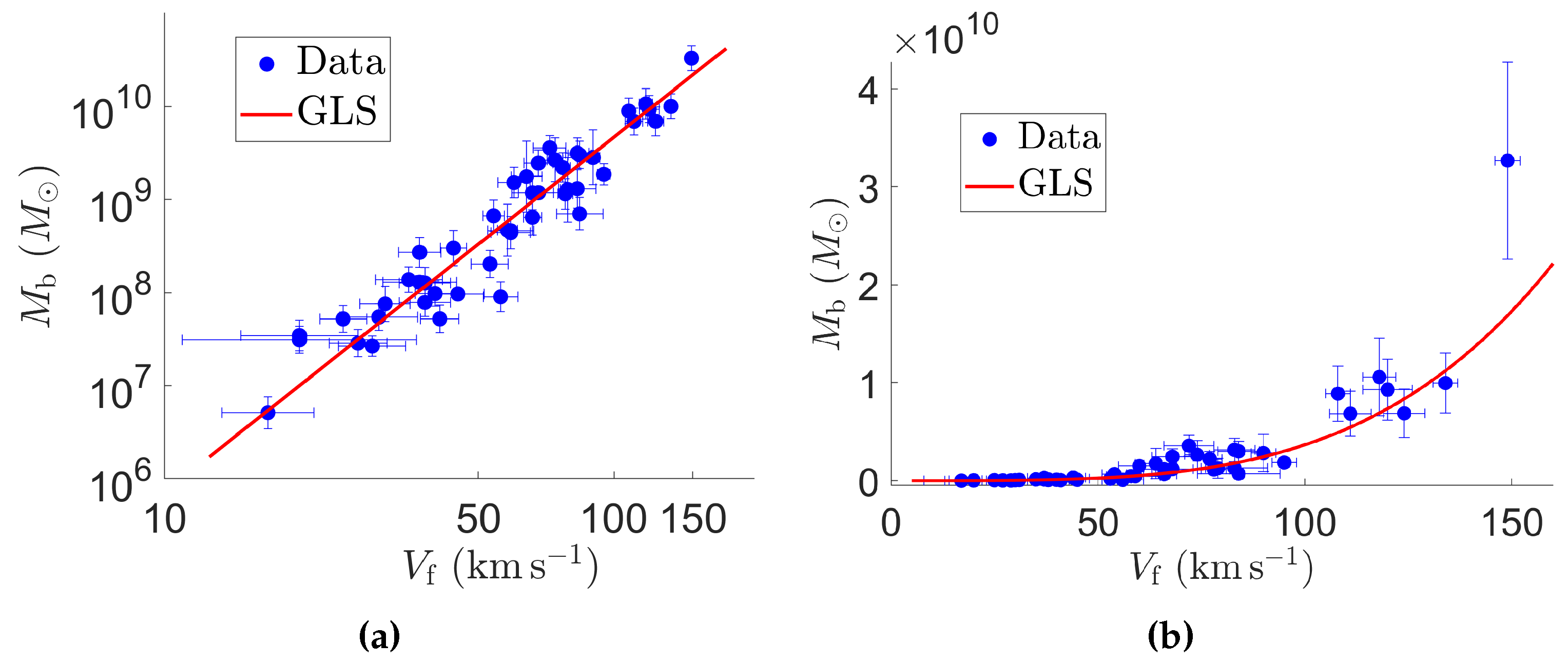
In this application, we demonstrate the robustness of GLS against outliers, by comparing between the loglinear and nonlinear regression of the BTFR. The scalings obtained with GLS are shown in Figure 3, reflecting consistent estimates for both regressions. In particular, whereas the data point corresponding to the largest V f and M b does not have the characteristics of an outlier on the logarithmic scale, it may be considered as such on the original scale. Nevertheless, the trend estimated by GLS seems not significantly affected by this outlier.
Furthermore, the relative error derived from the observed standard deviation estimated by GLS amounts to 63%, which is considerably larger than the value of ca. 40 % predicted by the model. Again, this is an indication that the scatter on the scaling law is not due to measurement error alone, which has particular significance in this application, as it may provide evidence for the Λ CDM vs. so-called modified Newtonian dynamics (MOND) cosmological models.

4.3. Visualization

It is interesting to visualize the data and the fit by GLS, as this provides insight into the way GLS succeeds in ignoring the outlier. This is illustrated in Figure 4, showing the Poincaré half-plane with the BTFR data, as well as the modeled and observed distributions obtained by GLS. The geodesic between the modeled outlier and the data point is shown (dashed curve), as well as that between the modeled outlier and the corresponding observed distribution (full curve). The latter is (slightly) shorter, because the increased observed standard deviation leads to a decrease in the geodesic distance.

5. Conclusions

Geodesic least squares regression has been presented, demonstrating the robustness of the method in two applications in the physical sciences. Essentially a least squares technique, it is easily implemented, which, as we have stressed, is a key asset for the adoption of the method in scientific disciplines where advanced methods of statistics and machine learning are not yet widely used. The data and results can be visualized in several ways, offering additional options for interpretation.
We have applied the GLS technique to the energy confinement scaling in fusion devices of the tokamak design based on an international multi-machine database. A new regression by GLS with a reduced set of predictor variables suggests an isotope effect that is much more favorable than predicted by regular MLE. This could lead to significantly improved confinement in the next-step fusion device ITER. A second application of GLS has been aimed at demonstrating the robustness against outliers, with a corresponding intuitive geometrical interpretation.
As GLS combines simplicity with good robustness properties, it can be of particular use for practitioners in various application domains. Requiring little to no tuning or learning of hyperparameters, it can be readily employed without expert knowledge about the details of the method.

Funding

This research received no external funding.

Institutional Review Board Statement

Not applicable.

Informed Consent Statement

Not applicable.

Data Availability Statement

The International Global H-mode Confinement Database is openly available here: https://osf.io/drwcq (accessed on 12 July 2023). The data used in this study to fit the Tully-Fisher scaling are available in [17].

Conflicts of Interest

The author declares no conflict of interest.

References

  1. Verdoolaege, G. A New Robust Regression Method Based on Minimization of Geodesic Distances on a Probabilistic Manifold: Application to Power Laws. Entropy 2015, 17, 4602–4626. [Google Scholar] [CrossRef]
  2. Amari, S.; Nagaoka, H. Methods of Information Geometry; American Mathematical Society: Providence, RI, USA, 2000. [Google Scholar]
  3. Nielsen, F. An elementrary introduction to information geometry. Entropy 2020, 22, 1100. [Google Scholar] [CrossRef] [PubMed]
  4. Burbea, J.; Rao, C. Entropy differential metric, distance and divergence measures in probability spaces: A unified approach. J. Multivar. Anal. 1982, 12, 575–596. [Google Scholar] [CrossRef]
  5. Von Toussaint, U. General Hyperplane Prior Distributions Based on Geometric Invariances for Bayesian Multivariate Linear Regression. Entropy 2015, 17, 3898–3912. [Google Scholar] [CrossRef]
  6. McCullagh, P.; Nelder, J. Generalized Linear Models; Chapman & Hall/CRC: Boca Raton, FL, USA, 1989. [Google Scholar]
  7. Rao, C.; Nagaoka, H. Differential metrics in probability spaces. In Differential Geometry in Statistical Inference; Amari, S.I., Barndorff-Nielsen, O.E., Kass, R.E., Lauritzen, S.L., Rao, C.R., Eds.; Institute of Mathematical Statistics: Hayward, CA, USA, 1987; Chapter 5; pp. 217–240. [Google Scholar]
  8. Beran, R. Minimum Hellinger distance estimates for parametric models. Ann. Stat. 1977, 5, 445–463. [Google Scholar] [CrossRef]
  9. Pak, R. Minimum Hellinger distance estimation in simple regression models; distribution and efficiency. Stat. Probab. Lett. 1996, 26, 263–269. [Google Scholar] [CrossRef]
  10. Freidberg, J. Plasma Physics and Fusion Energy; Cambridge University Press: Cambridge, UK, 2008. [Google Scholar]
  11. ITER Physics Expert Group on Confinement and Transport; ITER Physics Expert Group on Confinement Modelling and Database; ITER Physics Basis Editors. Chapter 2: Plasma confinement and transport. Nucl. Fusion 1999, 39, 2175–2249. [Google Scholar] [CrossRef]
  12. H-Mode Database Working Group. International Global H-Mode Confinement Database. 2021. Available online: https://osf.io/drwcq (accessed on 12 July 2023).
  13. Verdoolaege, G.; Kaye, S.M.; Angioni, C.; Kardaun, O.J.W.F.; Maslov, M.; Romanelli, M.; Ryter, F.; Thomsen, K.; the ASDEX Upgrade Team; the EUROfusion MST1 Team. The updated ITPA global H-mode confinement database: Description and analysis. Nucl. Fusion 2021, 61, 076006. [Google Scholar] [CrossRef]
  14. Xiao, X.; White, E.P.; Hooten, M.B.; Durham, S.L. On the use of log-transformations vs. nonlinear regression for analyzing biological power laws. Ecology 2011, 92, 1887–1894. [Google Scholar] [CrossRef] [PubMed]
  15. Maggi, C.; Weisen, H.; Hillesheim, J.C.; Chankin, A.; Delabie, E.; Horvath, L.; Auriemma, F.; Carvalho, I.S.; Corrigan, G.; Flanagan, J.; et al. Isotope effects on L-H threshold and confinement in tokamak plasmas. Plasma Phys. Control. Fusion 2018, 60, 014045. [Google Scholar] [CrossRef]
  16. Nielsen, F.; Nock, R. Visualizing hyperbolic Voronoi diagrams. In Proceedings of the 30th Annual Symposium on Computational Geometry (SOCG’14), Kyoto, Japan, 8–11 June 2014; pp. 90–91. [Google Scholar]
  17. McGaugh, S. The baryonic Tully-Fisher relation of gas-rich galaxies as a test of ΛCDM and MOND. Astron. J. 2012, 143, 40. [Google Scholar] [CrossRef]
Figure 1. Illustration of the Poincaré half-plane with several half-circle geodesics in the background. The confinement time data (value and error bar) are plotted in the half-plane, as well as the modeled and predicted values obtained by GLS.
Psf 09 00005 g001
Figure 2. (a) Visualization of the confinement time data on a pseudosphere, as well as the modeled and observed distributions obtained by GLS. (b) Projection of the confinement data using MDS, roughly indicating the directions of increasing μ and σ .
Psf 09 00005 g002
Figure 3. Fit of the BTFR by GLS (a) on a logarithmic scale and (b) on the original scale of the data.
Psf 09 00005 g003
Figure 4. The BTFR data in the Poincaré half-plane, with geodesics considered by GLS shown for the case of the outlier.
Psf 09 00005 g004
Table 1. Estimates of the parameters (intercept α 0 and exponents) and prediction toward ITER in power-law scalings with MLE and GLS of the energy confinement time using subsets of the DB5.2.3-STD5 database. All error bars correspond to one standard deviation.
α 0 α I α B α n α P α R α 1 + δ α κ α ϵ α M τ ^ E , th , ITER
MLE 0.0432 1.143 0.060 0.1914 0.7007 1.511 0.342 0.785 0.083 0.317 2.893
± 0.0014 ± 0.020 ± 0.017 ± 0.0097 ± 0.0075 ± 0.031 ± 0.046 ± 0.033 ± 0.049 ± 0.014 ± 0.034
GLS 0.0273 1.187 0.008 0.166 0.7511 1.485 0.509 0.823 0.365 0.767 2.996
± 0.0024 ± 0.024 ± 0.029 ± 0.015 ± 0.0089 ± 0.042 ± 0.060 ± 0.083 ± 0.087 ± 0.096 ± 0.057
Table 2. Estimates of the parameters (intercept α 0 and exponents) and prediction toward ITER in power-law scalings with MLE and GLS of the energy confinement time with a reduced set of predictor variables.
α 0 α I α P α R α M τ ^ E , th , ITER
MLE 0.0952 1.270 0.6194 1.182 0.570 2.717
± 0.0029 ± 0.012 ± 0.0079 ± 0.015 ± 0.026 ± 0.037
GLS 0.0280 1.124 0.6605 1.389 2.41 3.535
± 0.0028 ± 0.016 ± 0.0097 ± 0.019 ± 0.13 ± 0.098
Disclaimer/Publisher’s Note: The statements, opinions and data contained in all publications are solely those of the individual author(s) and contributor(s) and not of MDPI and/or the editor(s). MDPI and/or the editor(s) disclaim responsibility for any injury to people or property resulting from any ideas, methods, instructions or products referred to in the content.