Abstract
Using Bayesian inference to calibrate constitutive model parameters has recently seen a rise in interest. The Markov chain Monte Carlo (MCMC) algorithm is one of the most commonly used methods to sample from the posterior. However, the choice of which MCMC algorithm to apply is typically pragmatic and based on considerations such as software availability and experience. We compare three commonly used MCMC algorithms: Metropolis-Hastings (MH), Affine Invariant Stretch Move (AISM) and No-U-Turn sampler (NUTS). For the comparison, we use the Kullback-Leibler (KL) divergence as a convergence criterion, which measures the statistical distance between the sampled and the ‘true’ posterior. We apply the Bayesian framework to a Newtonian squeeze flow problem, for which there exists an analytical model. Furthermore, we have collected experimental data using a tailored setup. The ground truth for the posterior is obtained by evaluating it on a uniform reference grid. We conclude that, for the same number of samples, the NUTS results in the lowest KL divergence, followed by the AISM sampler and last the MH sampler.
1. Introduction
In the modeling of engineering problems, the governing equations usually consist of balance equations, such as the balance of mass, momentum and energy. These are known with absolute certainty. However, to obtain a tractable problem, parameterized constitutive equations are needed. These constitutive equations describe relations such as the ones between stress and strain in solid mechanics problems, stress and strain rate in fluid flow problems, and heat flow and temperature gradients in thermal problems. These constitutive equations are typically known with less certainty.
The selection and parameter estimation of constitutive laws is typically performed using well-defined lab experiments. In viscous flow problems, for example, we typically determine the constitutive model through rheological measurements, where we study the deformation of a soft solid or liquid in a well-defined flow. However, as engineering systems become more complex, the selection and parameter estimation of constitutive models becomes increasingly difficult. Bayesian inference is a powerful framework for addressing this issue. In Bayesian inference, model parameters are described probabilistically and are updated as new data become available [1,2], allowing for a systematic integration of prior knowledge and experimental data. Currently, Bayesian inference is still in its infancy in constitutive modeling, although it has recently seen an increase in interest. Some examples include determining the heat conductivity in a thermal problem [3], rheological parameters in non-Newtonian fluid mechanics [4,5], and constitutive modeling in biomaterials [6], elasto-viscoplastic materials [7], and elastic materials [8].
To infer the probability distribution of the parameters of a constitutive model, also referred to as the posterior, Markov chain Monte Carlo (MCMC) sampling methods are commonly used. Many different variants of MCMC are available, and researchers typically choose a sampling method based on pragmatic arguments such as software availability and experience. However, this might not always lead to an optimal choice in terms of sampler robustness, accuracy and efficiency.
A recent comparison of MCMC samplers based on a synthetically manufactured problem was presented by Allison and Dunkley [9], who considered the number of likelihood evaluations as the primary indicator for the performance of the samplers. In this contribution, we study the performance of various Bayesian samplers for a physical problem with real experimental data, viz., a squeeze flow. This problem considers the viscous flow of a fluid compressed in between two parallel plates. We herein consider a Newtonian fluid, for which the squeeze flow problem has an analytical solution [10]. We use the experimental data gathered with the tailored setup developed in Ref. [4]. For our comparison, we investigate three MCMC samplers: Metropolis–Hastings (MH), Affine Invariant Stretch Move (AISM) and No-U-Turn Sampler (NUTS). We study the convergence of these samplers through the Kullback–Leibler (KL) divergence to monitor the statistical distance between the sampled and the ‘true’ posterior [11].
This paper is structured as follows. In Section 2, we discuss the squeeze flow model, the experiments, and our prior information about the model parameters. The sampling methods to be compared are introduced in Section 3. The KL divergence is then discussed in Section 4, after which the performance of the samplers in the context of the squeeze flow problem is studied in Section 5. Conclusions are finally drawn in Section 6.
2. Constitutive Modeling of a Squeeze Flow
We consider a squeeze flow, which is a type of flow where a fluid is compressed between two parallel plates (Figure 1). In Ref. [4], we have developed a (semi-)analytical model and a tailored experimental setup to perform a Bayesian uncertainty quantification for a squeeze flow. In this section, we briefly discuss the squeeze flow model, the experiments, and the prior distributions chosen for the model parameters.
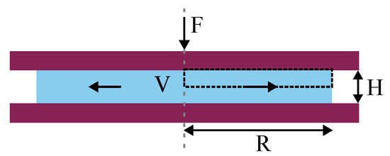
Figure 1.
Schematic of the squeeze flow, where two parallel plates (dark red) compress a fluid with volume V (light blue) by applying a force F. The distance between the parallel plates H and the radius of the fluid layer R evolve over time. The model domain is denoted by the dashed black box.
2.1. Analytical Model
In viscous problems, we analyze the flow behavior of a material by solving the mass and momentum balance, written as, respectively,
where is the velocity field, p the pressure field and the extra stress, which are all evolving in time. To relate the material’s response to its deformation, we assume a Newtonian constitutive equation, which yields an expression for as
where is the viscosity parameter and is the rate-of-deformation tensor, i.e., the symmetric gradient of the velocity field.
For the squeeze flow problem, we can assume the problem to be axisymmetric around the vertical axis, which is illustrated by the dashed gray line in Figure 1. Furthermore, due to the height of the fluid layer being much smaller than the radius of the fluid layer (), the lubrication approximation holds. Under these assumptions, an analytical solution for the radius of the fluid layer as a function of time can be found [10]:
In this expression, , F and V are the initial radius of the fluid, the applied force and the fluid volume, respectively. We refer the reader to Ref. [4] for the derivation of this analytical solution.
2.2. Experiments
The observations, which we denote by , are based on real data obtained by performing experiments on a squeeze flow setup. In Figure 2, we show the experimental setup, an image of the fluid layer during an experiment, and the processed data for (the measurement points, , are indicated by the solid black markers). We performed the experiment using liquid glycerol obtained from VWR Chemicals with purity ≥ 99.5%. It had been exposed to air for two days to be saturated with water absorbed from the air. We monitored the evolution of the fluid front for five minutes, from which we obtained our data to calibrate the squeeze flow model. The experiment was performed ten times, from which a mean and standard deviation for the radius were determined. See Rinkens et al. [4] for details regarding the setup and the experiments.
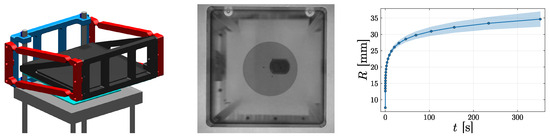
Figure 2.
(Left) Tailored experimental squeeze flow setup consisting of two transparent polymethylmethacrylate (PMMA) plates (cyan) in between which a fluid is compressed. We make use of parallel leaf springs (red) to ensure parallel motion of the PMMA plates and there is a camera beneath the aluminium frame (light gray). (Middle) The fluid front captured with the camera during an experiment. (Right) The aggregated data obtained from repeated experiments, visualized by .
2.3. Bayesian Inference
For the considered Newtonian flow case, we calibrate four model parameters, , based on the experimental data using Bayesian inference. The posterior probability density function, , of the parameters is effected by both the prior information of these parameters, , and the observations, , in accordance with Bayes’ rule
where is a normalization constant referred to as the evidence. The likelihood, which integrates the observations , is given by ().
The prior information for the parameters of interest is obtained through additional experiments. We retrieve the prior information on by measuring the simple shear response by performing steady rate sweep tests on a TA Instruments ARES rotational rheometer using a 25 mm diameter cone-plate geometry. To determine a prior for F, we measure the force using a spring suspension placed on the top part of the setup. We do not position additional weights on the setup, meaning that the applied force pertains to the weight of the top part of the setup. The fluid volume is measured separately by weighing a sample and multiplying it with the known density. The distribution for each of the priors has been determined by measuring them ten times, from which a mean and standard deviation are obtained. On account of the non-negativity of the volume, the initial radius and the viscosity, log-transforms are considered for these parameters, effectively resulting in a log-normal representation of their priors [4]. We list , and the coefficient of variation () of the prior distribution for each of the parameters in Table 1.

Table 1.
Statistics of the prior distributions for all model parameters.
3. Markov Chain Monte Carlo (MCMC) Samplers
Markov chain Monte Carlo (MCMC) samplers can be used to generate samples of the posterior distribution through stochastic simulation. The (statistics of the) model parameters can then be inferred from a simulated Markov chain [1,12], i.e., a stochastic process in which, given the present state, past and future states are independent [12]. If a Markov chain, independently of its initial distribution, reaches a stage that can be represented by a specific distribution, , and retains this distribution for all subsequent stages, we say that is the limit distribution of the chain [12]. In the Bayesian approach, the Markov chain is obtained in such a way that its limit distribution coincides with the posterior. More details about Markov chains for Bayesian inference can be found in the literature, e.g., Ref. [12].
We consider herein three different MCMC samplers: Metropolis–Hastings (MH), Affine Invariant Stretch Move (AISM) and No-U-Turn Sampler (NUTS). We aim to understand their advantages and disadvantages for the inference of the constitutive behavior of the squeeze flow. The considered solvers, as illustrated in Figure 3, are discussed in the remainder of this section.
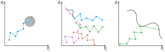
Figure 3.
Schematic of the three different MCMC samplers, where we assume to infer two parameters ( and ): (Left) MH: The chain is given in blue and the proposal distribution at the last step is denoted by the black circles. (Middle) AISM: For a two-parameter domain, we require (at least) four chains which are colored blue, orange, green and purple. We extrapolate the current position of a chain (purple) using the most recent state of another chain (blue). (Right) NUTS: The chain is denoted in green and the next step is determined by following the gradient of the posterior (black) through the current step.
3.1. Metropolis–Hastings (MH)
The first MCMC method we use is the Metropolis–Hastings (MH) algorithm [13,14]. We consider this algorithm because it is easy to implement and widely used for the estimation of parameters [1,2]. The MH algorithm starts with the definition of an initial guess for the vector of parameters. The parameter space is then explored by performing a random walk, in which the new candidate for the vector of parameters is sampled from a proposal distribution. This proposal is typically chosen to be a multivariate normal distribution, with its mean centered at the current state. The new candidate is then either accepted or rejected according to a probabilistic criterion. This procedure is repeated to generate the Markov chain.
The performance of the MH sampler is strongly influenced by the choice of the proposal covariance matrix, making careful selection a necessity. To objectively and optimally determine the proposal covariance, in the remainder of this work we employ the adaptive MCMC algorithm proposed by Haario et al. [15].
3.2. Affine Invariant Stretch Move (AISM)
The Affine Invariant Stretch Move (AISM) method is based on the algorithm developed by Goodman and Weare [16]. In this method, one uses multiple chains (also known as walkers) to explore the parameter space, where the number of walkers should be at least twice the number of parameters. The algorithm starts by defining an initial guess for each of the walkers, here sampled from the prior distribution. To explore the parameter space, the proposal for each walker (k), , is based on the current step, , of another randomly chosen walker (j) through linear extrapolation: . The extrapolation factor, Z, is sampled from a distribution with density
where the parameter has a default value , which is used in this work.
The number of walkers, to be selected by the user, can effect the performance of the sampler. To ensure objectivity of our comparison study, the sensitivity of the results to the number of walkers has been studied. The results of this sensitivity study convey that the results are rather insensitive to the number of samplers.
3.3. No-U-Turn Sampler (NUTS)
The No-U-Turn Sampler (NUTS) belongs to the class of Hamiltonian Monte Carlo (HMC) algorithms [17], which explore the parameter space using information from the gradient of the posterior. An advantageous feature of the NUTS sampler is that it automatically adapts its step size while exploring the parameter space [18], avoiding the need for the user to specify sampler parameters. The new candidate for the vector of parameters is selected according to the “No-U-Turn” criterion, which is based on the observation that the trajectory of the candidate often reverses direction when it encounters regions of high posterior density [18]. The sampler terminates the trajectory when it detects that the new candidate is starting to turn back on itself, indicating that further exploration is unlikely to yield better samples [18]. By continuously evaluating the gradient and the direction of the trajectory, NUTS can provide a more efficient exploration of the parameter space when compared to random-walk-based methods [18] such as the MH algorithm.
From the three samplers considered in this work, NUTS is the only one which requires gradient information of the model. In this work, we obtain the gradient with the forward mode automatic differentiation method [19]. This method allows for automatic differentiation of the considered analytical model. Although this increases the computational effort involved in the evaluation of the model, in terms of implementation no additional work is required.
4. Kullback–Leibler Divergence-Based Convergence Analysis
In this paper, we study the convergence behavior of the sampling algorithms discussed above. There are numerous possibilities for a convergence criterion for MCMC sampling methods, for example, the Gelman–Rubin statistic, the Geweke diagnostic, or the cross-correlation diagnostic [20,21,22]. We herein study convergence based on the Kullback–Leibler (KL) divergence, which provides a rigorous definition for the statistical distance between two probability distributions.
Given two probability distributions for a continuous random vector , P and Q, the KL divergence from P to Q is defined by
where and are the probability density functions for P and Q, respectively. In Figure 4 (left), we illustrate the concept of the KL divergence for a scalar-valued continuous variable by comparing two different probability density functions ( and ) to a reference distribution (q). In the illustrated case, the KL divergence is smaller than . The KL divergence is non-negative and only zero when a distribution is identical to the reference distribution.
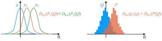
Figure 4.
Illustration of the KL divergence: (Left) The reference solution q is compared to two probability density functions and . (Right) The KL divergence can also be computed between two histograms.
In practice, it is convenient to approximate the KL divergence (6) through binning. Denoting the set of bin centers by , the KL divergence can be computed as
where and are the probabilities assigned to bin i for the distributions P and Q, respectively. Provided that the bins (both locations and sizes) are selected appropriately, the discrete KL divergence can be expected to resemble the divergence of the underlying continuous distributions; see Figure 4 (right).
In the case of sampling methods, it is natural to consider a binned discrete representation of the sampled distribution. Therefore, the discrete version of the KL divergence (7) will be considered in the remainder of this work. When we consider continuous distributions, we determine the bin probability as the product of the probability density in the bin center and the “volume” of the bin, and normalize the discrete distribution.
5. Comparison of the Samplers
With the squeeze flow problem and KL divergence measure introduced, the samplers can now be compared. In this section, we will first specify essential details regarding the comparison, after which we will present and discuss the comparison results.
5.1. Specification of the Comparison
To compare the sampling algorithms, we have to define a ‘true’ posterior used as the reference probability distribution. For this, we evaluate the posterior on a rectilinear grid in the parameter space, with the bounds for each parameter taken as . The mean and standard deviation used for these bounds have been determined through overkill sampling using 409,600 samples (excluding the burn-in period), the results of which are listed in Table 2.
Table 2.
The mean and standard deviation of the posterior for each sampler based on 409,600 samples excluding the burn-in period.
To attain insight into the quality of the rectilinear reference grid, we have created three different grid structures, enclosed by . Each of the four parameter ranges is divided into 27, 9 or 3 cells, resulting in , and bins, respectively. In each bin, the posterior is evaluated by multiplying the likelihood and the prior and subsequently normalizing it. To compare the sampled posterior to the reference grid, we divide the number of samples within a bin and divide it by the total number of samples collected in all bins. In the exceptional case that samples fall outside the boundaries of the reference domain, these are not taken into account in the total number of samples.
5.2. Results of the Comparison
To provide a frame of reference for the KL divergence comparison, in Figure 5, the divergence of the prior distribution from the reference posterior distribution based on bins is shown (dot–dashed line). It is observed that the divergence of the posterior computed on the one-time coarsened grid ( bins) and on the two-times coarsened grid ( bins) is substantially smaller than that for the prior (dashed lines), indicating that the rectilinear grid approximation on the finest reference grid ( bins) provides a high-quality approximation of the posterior.
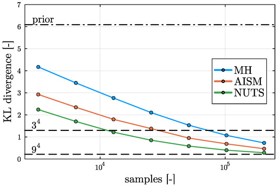
Figure 5.
KL divergence behavior of the different sampling methods. All KL divergences are defined with respect to the reference grid ( bins). The KL divergence of the prior and coarsened rectilinear grids are shown to provide a frame of reference.
From Figure 5, it is observed that all three samplers decrease the error monotonically, demonstrating the robustness of all three solvers. Asymptotically, the KL divergence is expected to approach a finite (but small) value corresponding to the divergence from the exact posterior to the reference grid with bins. We observe that the MH sampler has the largest distance from the reference for a fixed value of the sample size. Despite the fact that the AISM sampler does not require additional information from the model, for the considered problem, this sampler explores the parameter space more efficiently than the MH sampler, despite the optimized selection of the MH proposal covariance. The NUTS results are observed to significantly outperform the AISM sampler. This conveys that the gradient information used by NUTS effectively improves the exploration of the parameter space.
Figure 5 also shows that for the relatively small number of parameters considered in this problem, the evaluation of the posterior on equidistant grids is very efficient. Specifically, the results obtained on the intermediate grid (6561 evaluations for bins) outperforms all samplers for the maximum considered sample size (4.096 · 105 samples). We stress that this observation is very specific to the case of a small number of parameters [23], and that for problems with more parameters, evaluation of the posterior on rectilinear grids becomes quickly intractable.
6. Conclusions
A comparison of three commonly used MCMC samplers is presented for the Bayesian uncertainty quantification of a Newtonian squeeze flow. The Bayesian inference of the model parameters is based on experimental data gathered through a tailored setup. The Kullback–Leibler (KL) divergence is used to study the convergence of the different samplers.
It is observed that the KL divergence decreases monotonically for all samplers, and that all samplers converge toward the exact posterior. The No U-Turn Sampler (NUTS) is observed to result in the best approximation of the posterior for a given sample size, which we attribute to the gradient information used by this sampler. The Affine Invariant Stretch Move (AISM) sampler, which does not require gradient information, is found to yield a substantial improvement in exploring the parameter space compared to the Metropolis–Hastings algorithm.
In this study, we have limited ourselves to the KL divergence as a measure for convergence. The comparison of this convergence measure to other criteria will be considered in future work. The comparison can also be improved further by taking the computational effort into consideration. This will, for example, take into account the increase in computational effort involved in evaluating gradients for the NUTS solver. Furthermore, extending the physical problem under consideration to more complex cases (with more model parameters) will provide insights regarding how such extensions affect the sampler comparison.
Author Contributions
Conceptualization, A.R., R.L.S.S., N.O.J., E.Q. and C.V.V.; methodology, A.R., R.L.S.S., E.Q. and C.V.V.; software, A.R. and R.L.S.S.; validation, A.R. and R.L.S.S.; formal analysis, A.R., R.L.S.S., E.Q. and C.V.V.; investigation, A.R. and R.L.S.S.; data curation, A.R. and R.L.S.S.; writing—original draft preparation, A.R. and R.L.S.S.; writing—review and editing, A.R., R.L.S.S., C.V.V., N.O.J. and E.Q.; visualization, A.R. and R.L.S.S.; supervision, C.V.V., N.O.J. and E.Q.; project administration, C.V.V., E.Q. and N.O.J. All authors have read and agreed to the published version of the manuscript.
Funding
This research was funded directly by the Eindhoven University of Technology.
Institutional Review Board Statement
Not applicable.
Informed Consent Statement
Not applicable.
Data Availability Statement
The experimental data can be found on Github: https://github.com/s152754/PhDproject/tree/main/Squeezeflow/Experiments/RoutExp (accessed on 19 September 2025).
Acknowledgments
This research was partially conducted as part of the DAMOCLES project within the EMDAIR program of the Eindhoven Artificial Intelligence Systems Institute (EAISI).
Conflicts of Interest
The authors declare no conflicts of interest.
References
- Kaipio, J.; Somersalo, E. Statistical and Computational Inverse Problems; Springer Science & Business Media: New York, NY, USA, 2006; Volume 160. [Google Scholar]
- Ozisik, M.N. Inverse Heat Transfer: Fundamentals and Applications; Routledge: New York, NY, USA, 2018. [Google Scholar]
- Silva, R.L.; Verhoosel, C.V.; Quaeghebeur, E. Bayesian estimation and uncertainty quantification of a temperature-dependent thermal conductivity. arXiv 2024, arXiv:2403.12696. [Google Scholar] [CrossRef]
- Rinkens, A.; Verhoosel, C.V.; Jaensson, N.O. Uncertainty quantification for the squeeze flow of generalized Newtonian fluids. J.-Non-Newton. Fluid Mech. 2023, 322, 105154. [Google Scholar] [CrossRef]
- Kim, J.; Singh, P.K.; Freund, J.B.; Ewoldt, R.H. Uncertainty propagation in simulation predictions of generalized Newtonian fluid flows. J. Non-Newton. Fluid Mech. 2019, 271, 104138. [Google Scholar] [CrossRef]
- Akintunde, A.R.; Miller, K.S.; Schiavazzi, D.E. Bayesian inference of constitutive model parameters from uncertain uniaxial experiments on murine tendons. J. Mech. Behav. Biomed. Mater. 2019, 96, 285–300. [Google Scholar] [CrossRef] [PubMed]
- Chakraborty, A.; Messner, M.C. Bayesian analysis for estimating statistical parameter distributions of elasto-viscoplastic material models. Probabilistic Eng. Mech. 2021, 66, 103153. [Google Scholar] [CrossRef]
- Rappel, H.; Beex, L.A.; Hale, J.S.; Noels, L.; Bordas, S. A tutorial on Bayesian inference to identify material parameters in solid mechanics. Arch. Comput. Methods Eng. 2020, 27, 361–385. [Google Scholar] [CrossRef]
- Allison, R.; Dunkley, J. Comparison of sampling techniques for Bayesian parameter estimation. Mon. Not. R. Astron. Soc. 2014, 437, 3918–3928. [Google Scholar] [CrossRef]
- Engmann, J.; Servais, C.; Burbidge, A.S. Squeeze flow theory and applications to rheometry: A review. J. Non-Newton. Fluid Mech. 2005, 132, 1–27. [Google Scholar] [CrossRef]
- Kullback, S.; Leibler, R.A. On information and sufficiency. Ann. Math. Stat. 1951, 22, 79–86. [Google Scholar] [CrossRef]
- Gamerman, D.; Lopes, H.F. Markov Chain Monte Carlo: Stochastic Simulation for Bayesian Inference; Chapman and Hall/CRC: New York, NY, USA, 2006. [Google Scholar]
- Metropolis, N.; Rosenbluth, A.W.; Rosenbluth, M.N.; Teller, A.H.; Teller, E. Equation of state calculations by fast computing machines. J. Chem. Phys. 1953, 21, 1087–1092. [Google Scholar] [CrossRef]
- Hastings, K.W. Monte Carlo sampling methods using Markov chains and their applications. Biometrika 1970, 57, 97–109. [Google Scholar] [CrossRef]
- Haario, H.; Saksman, E.; Tamminen, J. An adaptive Metropolis algorithm. Bernoulli 2001, 7, 223–242. [Google Scholar] [CrossRef]
- Goodman, J.; Weare, J. Ensemble samplers with affine invariance. Commun. Appl. Math. Comput. Sci. 2010, 5, 65–80. [Google Scholar] [CrossRef]
- Neal, R.M. MCMC using Hamiltonian dynamics. arXiv 2012, arXiv:1206.1901. [Google Scholar] [CrossRef]
- Hoffman, M.D.; Gelman, A. The No-U-Turn sampler: Adaptively setting path lengths in Hamiltonian Monte Carlo. J. Mach. Learn. Res. 2014, 15, 1593–1623. [Google Scholar]
- Baydin, A.G.; Pearlmutter, B.A.; Radul, A.A.; Siskind, J.M. Automatic differentiation in machine learning: A survey. J. Mach. Learn. Res. 2018, 18, 1–43. [Google Scholar]
- Cowles, M.K.; Carlin, B.P. Markov chain Monte Carlo convergence diagnostics: A comparative review. J. Am. Stat. Assoc. 1996, 91, 883–904. [Google Scholar] [CrossRef]
- Roy, V. Convergence diagnostics for markov chain monte carlo. Annu. Rev. Stat. Its Appl. 2020, 7, 387–412. [Google Scholar] [CrossRef]
- Geweke, J. Evaluating the Accuracy of Sampling-Based Approaches to the Calculation of Posterior Moments; Technical Report; Federal Reserve Bank of Minneapolis: Minneapolis, MN, USA, 1991. [Google Scholar]
- Smith, R.C. Uncertainty Quantification: Theory, Implementation, and Applications; Society for Industrial and Applied Mathematics: Philadelphia, PA, USA, 2013. [Google Scholar]
Disclaimer/Publisher’s Note: The statements, opinions and data contained in all publications are solely those of the individual author(s) and contributor(s) and not of MDPI and/or the editor(s). MDPI and/or the editor(s) disclaim responsibility for any injury to people or property resulting from any ideas, methods, instructions or products referred to in the content. |
© 2025 by the authors. Licensee MDPI, Basel, Switzerland. This article is an open access article distributed under the terms and conditions of the Creative Commons Attribution (CC BY) license (https://creativecommons.org/licenses/by/4.0/).