Abstract
Concentrating solar power (CSP) is a high-potential renewable energy source that can leverage various thermal applications. CSP plant development has therefore become a global trend. However, the designing of a CSP plant for a given solar resource condition and financial situation is still a work in progress. This study aims to develop a mathematical model to analyze the levelized cost of electricity (LCOE) of Thermal Energy Storage (TES)-integrated CSP plants in such circumstances. The developed model presents an LCOE variation for 18 different CSP configurations with TES incorporated for Rankine, Brayton, and combined power generation cycles, under regular TES materials and nano-enhanced TES materials. The model then recommends the most economical CSP plant arrangement. Within the scope of this study, it was found that the best configuration for electricity generation is a solar power tower with nano-enhanced phase change materials as the latent heat thermal energy storage medium that runs on the combined cycle. This returns an LCOE of 7.63 ct/kWh with a 22.70% CSP plant efficiency. The most favorable option in 50 MW plants is the combined cycle with a regular TES medium, which has an LCOE of 7.72 ct/kWh with a 22.14% CSP plant efficiency.
1. Introduction
Concentrating solar power (CSP) is a technology that uses mirrors or lenses to reflect sun rays into a focal point (or line), allowing thermal energy to accumulate in a material with good heat storage capability. This concentrated thermal energy can be used to drive various thermal applications. Among those applications of CSP are electricity generation, district heating systems, industrial process heating, water desalination, etc. [1,2]. The primary significance of CPS is that it is a clean energy source with a meager contribution to greenhouse gas emissions throughout the life cycle of the CSP plant, especially when compared to conventional fossil fuel energy sources [3]. Moreover, fossil fuels reserves are depleting, and their supply can be disrupted due to various geopolitical phenomena, necessitating the search for more sustainable energy solutions to power humanity. CSP plants are classified into four types: parabolic trough (PT), solar power tower (SPT), parabolic dish (PD), and linear Fresnel (LF) [4]. The performance parameters such as concentration, operational temperature range, efficiency, capacity, costs, and land use vary depending on these configurations [5]. The PT configuration is the most commonly used CSP configuration, followed by the SPT configuration, due to their superior performance under the aforementioned factors [6]. Since solar energy is inherently intermittent due to its dependence on the diurnal cycle and climate conditions, all CSP plants, regardless of configuration, require a thermal energy storage (TES) system to maintain the balance of demand and supply [7].
TES, where excess energy is stored in a thermal reservoir using a storage medium, is most suited to this type of application due to its cost-effective and efficient operation compared to other energy storage types available. Consequently, the main purpose of a TES system can be identified as storing heat energy when the sun is available and utilizing the stored energy to operate a thermal cycle when the sun is unavailable. As a result, TES ensures that the CSP plant continues to operate at a lower cost while also providing other benefits such as increased plant reliability, efficiency, energy savings, and annual capacity factor [8,9,10,11]. Sensible heat thermal energy storage (SHTES), latent heat thermal energy storage (LHTES), and thermochemical storage are the three main types of TES available [12]. SHTESs are designed to store heat energy as sensible heat of the working material, LHTES is designed for the latent heat of the physical phase transition of storage material, while some sensible heat is also efficiently stored, and thermochemical storage is designed to store thermal energy through a chemical reaction of storage materials [13]. Despite the fact that LHTES and thermochemical storage have higher energy density than SHTES, SHTES is the most commonly installed TES type, particularly in CSP power plants, due to its economic benefits and simplicity [14,15]. LHTES is less expensive than thermochemical storage and thus can be identified as the next potential candidate for CSP plants [16]. Furthermore, the performance of TES can be improved by upgrading the configuration, geometry and materials used. Improvement of the storage medium by encapsulation, modification of the chemical composition, and addition of micro-/nano-particles of foreign material are some of the more popular methods. The enhancement of thermo-physical properties of storage materials through the addition of nanoparticles has numerous success stories, as evidenced by previous literature [17,18,19].
Any of these TES systems can be integrated with a CSP plant in such a way that the TES system is always charged prior to delivering thermal energy to the application (active TES), and the TES system can be charged with excess thermal energy that is not required by the application (passive TES). In general, active TES consists of direct integration with the same storage medium as heat transfer fluid (HTF), whereas indirect integration uses two different materials as the storage medium and HTF [20]. Therefore, the optimal design of a CSP plant integrated with TES must be tailored to the situation while also taking into account the other system requirements. The levelized cost of energy (LCOE) is one such important design consideration in CSP plant design to predict economic competitiveness. With the recent drive towards decarbonization, CSP technologies have received increased attention, with numerous R&D contributions leading to a reduction of more than 50% of the LCOE of CSP plants [21]. As a result, CSP plant construction is accelerating, with the installed capacity of CSP expected to reach 22.4 GW by 2030 to utilize a larger portion of the total global CSP potential of 2,945,926 TWh/y [22]. The current global weighted average cost of CSP in electricity generation is approximately 0.108 USD/kWh, according to data from the International Renewable Energy Agency (IRENA) [23]. However, the LCOE is entirely dependent on the geographical location of the CSP plant and the regional macroeconomic conditions. As a result, it is worthwhile creating a systematic model that any project developer anywhere around the world can use in making CSP plant design and development decisions.
Aseri et al. [24] conducted a study on the techno-economic appraisal of 50 MW nominal capacity parabolic trough solar collector and solar power tower-based CSP plants with a provision of 6.0 h of TES at two potential locations in India for different condenser cooling options. Musi et al. [25] conducted a study to evaluate the LCOE of CSP plants, and the findings show a country- and technology-level learning effect for CSP plant LCOE. Furthermore, the construction of large CSP plants does not currently result in LCOE reductions, and LCOE reductions are generally positively correlated with greater thermal energy storage, a higher capacity factor, and, to a lesser extent, power output. Mahlangu et al. [26] conducted research to evaluate the external costs associated with a solar CSP plant using life cycle analysis. Some of the relevant studies in the open literature include Hussain et al. [27], who conducted a study that presented a cost analysis of a 20 MW concentrated solar power plant with a thermal energy storage system in Bangladesh. However, none of these studies provide a comprehensive outlook on the energy generation costs associated with CSP plants.
As a consequence, this comprehensive study is dedicated to identifying the parameters that affect the LCOE of CSP plants and developing an aggregated mathematical model that can be used in estimating the LCOE of future TES-integrated CSP plant designs prior to construction. Given the maturity of CSP and TES technologies, the work presented in this paper has chosen PT and SPT CSP configurations, shown in Figure 1, as well as SHTES and LHTES configurations, to be integrated into CSP plants as active indirect storage systems. Both SHTES and LHTES storage types are considered in a single-tank thermocline arrangement. All TES configurations are taken into account for both regular working materials and nano-enhanced storage materials. Furthermore, due to the high-temperature attainment of the SPT arrangement, in which the use of SHTES has less economic competitiveness, the SPT solar plant arrangement will be integrated only with the LHTES storage type. The use of phase transitions to increase storage energy density can drastically reduce storage material requirements and thus storage size and cost. The consideration of nanotechnology in CSP plants was evaluated depending on a hypothesis. Thermal energy is being used to generate electricity in three different power generation cycles: the Rankine cycle, the Brayton cycle, and the combined power cycle. Therefore, the research presented in this paper will contribute to the development of a mathematical model that is applicable for both PT and SPT configurations, as well as the identification and verification of LHTES in improving CSP plant performance over other available TES types. There was no previous study that considered all three power generation cycles considered in this study at the same time, and no attention was previously given to the evaluation of LCOE with the integration of nanoparticles into the TES medium.
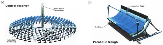
Figure 1.
Selected CSP plant configurations for the study: (a) solar power tower configuration (SPT) and (b) parabolic trough configuration (PT) [28].
2. Materials and Methods
It is obvious that different configurations of CSP and TES have different technical performance levels and thus economies. In general, incorporating TES into CSP plants can improve energy system performance while lowering LCOE [29,30]. However, the optimal configuration that delivers technology at an affordable price must be identified. Furthermore, the geographical location of the CSP plant strictly defines the LCOE through direct normal irradiance (DNI), capital expenditure (CAPEX), operational expenditure (OPEX), and a discount ratio that is dependent on the country’s economy. The current study, which is designed to evaluate the LCOE variation under various scenarios that include CSP, TES, and end-use single-stage thermal cycles, follows the main steps depicted in Figure 2. One scenario from each CSP configuration was chosen as the base case for comparing LCOE variation under the considered end-use thermal cycles in electricity generation, i.e., Rankine cycle, Brayton cycle, and combined cycle. The efficiencies of the thermal cycle (which depend on the plant’s operational temperatures and pressures), the efficiency of the TES (which depends on the TES configuration and nanoparticle addition for TES efficiency improvement) were considered, under an estimated DNI of 1000 kWh/m2/year and 50 MW of installed electric generation capacity with the unit solar multiplier. TES was designed to run the power plant without the sun for six hours. Under the same solar insolation, the regular TES-integrated plants were evaluated for LCOE variation under 50–100 MW of installed electricity generation capacity range. Furthermore, under the same solar insolation, the nano-enhanced TES-integrated plants were evaluated for an installed electricity generation capacity of 100 MW. The best-performing plant configurations of each PT and SPT were then selected to be located in various geographical locations, in order to vary the DNI level and identify the LCOE variation around the world in a future study.
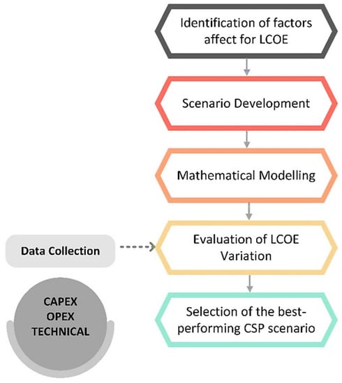
Figure 2.
Evaluation methodology for LCOE variation.
2.1. Factors Affecting the LCOE
LCOE is a metric which measures the average net present value of energy generation expenses over the life span of the energy system to a unit of energy produced. The LCOE can be calculated using Equation (1) [31], which takes into account both financial and technical factors. Therefore, the main factors defining the economy of the energy system are CAPEX (It), OPEX (Mt), fuel cost (Ft), discount ratio (r), plant life span (n), and energy generation (Et). There is no fuel cost associated with solar energy. As a result, in this case, fuel cost (Ft) = 0. Furthermore, this study does not take into account the costs of decommissioning CSP plants or natural degradation.
2.1.1. Cost Components of LCOE
Table 1 shows the CAPEX and OPEX components for a solar thermal power plant [32,33]. These components differ depending on the CSP and TES configurations. The discount rate is another economic factor that affects LCOE, and it is strictly dependent on the country’s economy, so the LCOE of CSP plants is subject to vary with the economy of the country where the plant is located. Further, the study was conducted with a 25-year life span [34] for a CSP plant with zero salvage value in order to evaluate the feasibility of CSP plants for selected countries in various geographical locations.

Table 1.
LCOE components identification.
The energy requirement for the end-use application determines the capacity of the CSP plant, as do the power block and TES. Once a specific solar collector is chosen for a CSP configuration, the number of solar collectors required is primarily determined by the power plant’s capacity. When DNI rises, the number of solar collectors required decreases, lowering CAPEX. The total land area required for the power plant (LAT) can be calculated using Equations (2) and (3) for PT and SPT, respectively [24], considering the unit area of solar collector (A1) and number of solar collectors in the field (N). Following that, the expenditure for the land (CL) is calculated as per Equation (4), considering the unit price of land area (PrL). The cost of solar collectors (CS), as per Equation (5), is based on the unit price of solar collectors (PrS) and N, while Equation (6) for the cost of TES is based on the storage material mass quantity (mSM), the unit price of storage medium (PrSM), container material mass quantity (mCM), the unit price of container material (PrCM) and cost of auxiliary (CAC).
A CSP plant’s typical equipment includes an HTF system (HTF, HTF tank, piping, insulation, and pumps), a solar field (mirrors, frame, foundation, sun tracking systems, and controllers), and a water treatment plant as the major auxiliary. TES system consists of storage material, tanks, piping, insulation, pumps, and heat exchangers. If the electricity is generated using the Rankine cycle, the power block consists of a steam generator, condenser, pump, and steam turbine. When considering the Brayton cycle, the gas turbine and compressor are present, whereas combined cycle power generation makes use of all of these components. In this study, the combined cycle is regarded as a topping cycle. Additionally, a cooling system and an electric generator are also required for the power block [33]. The cost components for the study’s three different power cycles are reported in Table 2 [35,36,37,38,39,40,41], while efficiencies and economies are reported in Table 3 [42], and storage medium costs are reported in Table 4. The balance of the system expenditure consists of the costs of heat exchangers, pumps, piping, fittings, and all other CSP system components that were not considered as separate cost components. CAPEX from solar collectors and TES was calculated using Equations (5) and (6), respectively. The efficiency of the combined cycle was calculated using Equation (43), while the cost of the combined cycle is simply the sum of individual cycle costs. According to Trevisan et al. [43], the expense of a Brayton cycle power generation system is three times that of a Rankine cycle used for power block cost estimation.
Table 2.
Cost components considered in LCOE estimating of PT and SPT plants.
Table 3.
Efficiency and costs for Rankine, Brayton and combined cycle for electricity generation.
Table 4.
Unit costs of different materials considered for TES.
2.1.2. Technical Components for LCOE
Efficiencies at each level of the CSP plant energy conversion impact the value of LCOE, as shown in Figure 3, and they bear the primary contribution in terms of annual energy generated. Mirror, receiver, HTF, and heat exchanger efficiency are the main components of energy loss in the CSP system. The efficiency of solar collectors is dependent on several factors, including cosine factor, spillage factor, attenuation factor, blocking factor, shadowing factor, and reflectivity [47]. The cosine factor is the most important of these. It is determined by the solar collector’s geometry. The portion of the radiation reflected by the mirrors that do not reach the receiver is referred to as the spillage factor. The attenuation factor addresses the energy loss caused by air molecule absorption in the region between the mirrors and the receiver, which increases the energy loss exponentially as the distance between the mirrors and the receiver increases. The energy lost when one heliostat casts a shadow on another is accounted for by the shadowing factor. Reflectivity is the product of nominal reflectivity and nominal cleanliness [32]. The efficiency of the receiver is also affected by reflectivity and environmental conditions. The HTF properties and the ambient temperature determine the piping loss. The CSP configuration, TES configuration, and materials used in these systems significantly impact energy transmission efficiency. The mirror arrangement in the solar field and solar collector efficiency define the amount of energy the CSP field can collect. As well as the effective surface area for heat loss, which is determined by the TES configuration and material choice, plays the main role in TES efficiency. Thermal cycle efficiency, turbine efficiency, and generator efficiency are all important. The power cycle type and operational conditions, such as temperature and pressure, determine the efficiency of a thermal cycle. Although some other losses are associated with TES-integrated CSP plants for electricity generation, the current study assumes that such losses are negligible. Table 5 shows the generalized efficiency values of the generator, heat exchanger, and HTF (solar salt) energy transmission losses in piping used for this study. Table 6 presents the TES material thermo-physical properties.
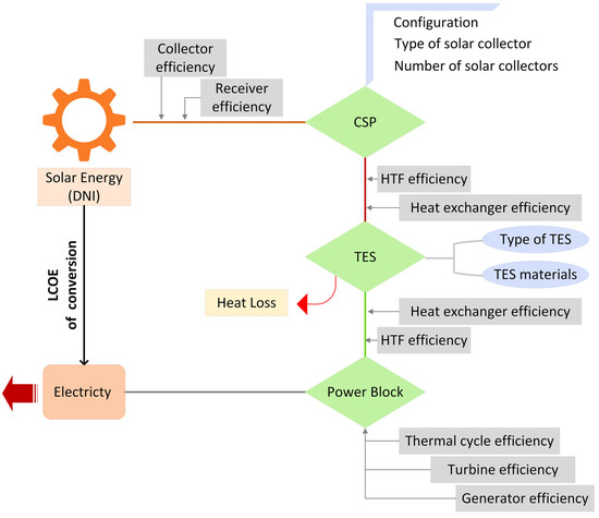
Figure 3.
Technical components that affect the LCOE of CSP plants.
Table 5.
Efficiencies of common system components of both PT and SPT power plants.
Table 6.
Thermophysical properties of the storage materials selected for TESs.
3. Scenario Development
As shown in Figure 4, this study considered 18 scenarios to evaluate the LCOE variation of TES-integrated CSP plants for electricity generation. Because of SPT’s high-temperature capability, this CSP configuration is only considered with LHTES. In contrast, the use of SHTES can improve the size and cost of the TES system due to the comparatively low energy density resulting from storing only sensible heat. When latent heat storage is neglected, TES requires more storage medium to store the same amount of energy, causing container size to increase. The single-stage Rankine cycle, Brayton cycle, and combined cycle were chosen as end-use thermal applications that use CSP power extract for both CSP configurations. Though combined cycle operation necessitates higher operational temperatures for efficiency, the PT configuration is also taken into account under PT configuration to check the economic feasibility of such a combination in CSP-based electricity generation.
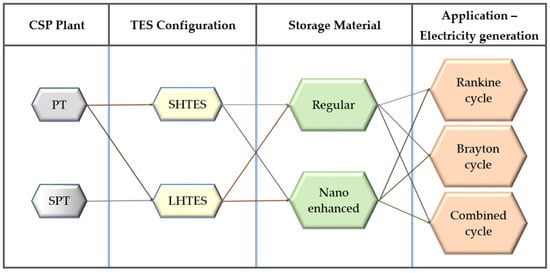
Figure 4.
Scenario development for LCOE evaluation.
4. Mathematical Modelling
Following the LCOE equation, this section develops a model to calculate the LCOE of the energy generated by the CSP plant. As shown in Equation (7), the energy generated by the CSP plant (Et) is dependent on the DNI at the plant’s location (latitude and longitude), unit area of solar collector (A1), number of solar collectors (N), the efficiency of solar collectors (ηcollector), the efficiency of the solar receiver (ηreceiver), HTF efficiency (ηHTF), heat exchanger (HE) efficiency (ηHE), number of heat exchangers (NHE), efficiency of TES system (ηTES), thermal cycle efficiency (ηthermal), turbine efficiency (ηT) and electricity generator efficiency (ηG). All other system component losses are assumed to be insignificant. In the current study, the efficiency of the receiver, heat exchangers, HTF, and generator was assumed to be constant for each of the selected configurations using industry-standard values. As a result, Equation (7) can be reduced to Equation (8). In the event that the plant is assumed to have only two mandatory heat exchangers (NHE = 2) required for the TES system to mount with the CSP plant in an active indirect manner. The unit area of a solar collector is accounted for using a standard solar collector available on the market, resulting in a constant for a chosen CSP configuration. The spacing between collectors varies depending on the solar collector, and therefore, the collector efficiency varies as well. Other factors influencing collector and receiver efficiency mainly include construction geometry and materials. Once the solar collector is chosen for the specific CSP plant, the number of solar collectors required is determined by the available DNI level and the end-use application energy demand. The land requirement for a solar field varies depending on the number of solar collectors, causing plant costs to vary proportionally.
Solar collectors will not capture total incident DNI on the solar field, since collector efficiency is not 100%. To determine the actual energy collected by SPT collectors (PT), Equation (9), derived from Equations (10) and (11), can be used [32,47]. Equation (12) is used for PT plant collectors as other components that affect efficiency are considered under receiver efficiency. Here, DNI is related to the location selected which the current study considers 1000 kWh/m2/year of the bottom line. Ai is the solar collector area of the ith collector, θi is the angle between the incident solar rays and normal to ith mirror element, fsp,i is the spillage factor, fat,i is the attenuation factor, fb is the blocking factor, fsh is the shadowing factor, αc is the reflectivity, and foptical is the factor for optical efficiency.
Accordingly, the efficiency of collector in SPT plant can be derived as;
Furthermore, in addition to the cosine factor, fat,i is critical in SPT plants because as the plant grows larger, the loss increases, and it can be found as follows using Equation (13) or (14) depending on the size of the solar plant, where D is the distance between the solar collector and the focal point of the receiver. The shadowing factor and spillage factor in this study was taken as constant values where more realistic values for these factors can be calculated as per Talebizadeh et al. [51]. Hussaini et al. conducted a study that considered 0.88 of nominal reflectivity and 0.98 cleanliness over the entire life span, resulting in αc = 0.84 [52], considered in collector efficiency estimation in this study.
SPT receiver efficiency (ηreceiver) can be calculated as per Equation (15) [53], while the PT receiving efficiency is directly considered the same as the HTF efficiency. The current study has no consideration of conductive heat transfer loss. Here, qin,HTF is the solar power transferred to HTF, qsolar incident is the incident solar power on the receiver, and qloss,receiver is the heat loss in the receiver.
Receiver heat loss mainly consists of two losses, as shown in equation 16: the radiation heat loss (qrad) and the convection heat loss (qconv).
Radiation heat loss of the receiver can be calculated as per Equation (17), considering the radiation shape factor of the receiver (SF), which the presented study considered to be SF = 1, the radiative area of the receiver (AR), the emissivity of the receiver (ε), the Stefan Boltzmann constant (σ = 5.67037442 × 10⁻⁸ kg s−3 K−4), the receiver temperature (TR), and the ambient temperature (Tambient).
Convection heat loss of the receiver can be found by Equation (18), where hconv is the convective heat transfer coefficient, which can be calculated by Equation (19), and HR is the total height of the receiver.
The effectiveness of the receiver determines heat transfer from the receiver to the HTF. Essentially, the efficiency at the receiver is primarily determined by the receiver’s reflectivity and the conduction and convection heat transfer coefficients, which are used to calculate thermal energy loss to the environment. The efficiency of the receiver is also subject to natural degradation over time, and cleanliness is another major parameter that influences these efficiencies. Assuming that this decay is negligible for the lifespan of the CSP plant receiver, it will be treated as a constant value for each configuration, as shown in Table 5.
The efficiency of the HTF (ηHTF) is primarily determined by environmental factors such as ambient temperature (Tambient), humidity, and airflow velocity at the geographical location. Despite this, the HTF chosen for the study is solar salt with a chemical composition of 40 wt.% KNO3+ 60 wt.% NaNO3 for the PT plant and KCl/MgCl2/NaCl for the SPT plant is considered under a constant efficiency value, as shown in Table 5. The TES system is critical in CSP plants for improving overall energy system performance while lowering energy costs. The storage material, container material, insulation, environmental conditions, and geometric configuration of a TES all impact its efficiency. In this study, Equation (20) is used to estimate the efficiency of TES (ηTES) [54], where ETES is the energy stored in the TES, qout,HTF is thermal energy output from the HTF to TES, and Eloss,TES is the thermal energy loss from TES.
Therefore, the thermal energy loss from the TES can be found by Equation (21), considering the overall heat transfer coefficient (UTES), heat transfer area of the TES (Aht), and TES outlet temperature (TTES).
The heat transfer area of the TES can be then calculated using Equation (22), considering DTES as the diameter of the TES and H as the height of the TES.
The amount of heat energy that can be stored in SHTES and LHTES is given by the following equations, Equations (23) and (24), respectively, assuming the negligible heat storage in the components inside of TES [55,56]. Here, ESHTES is the amount of heat energy that can be stored in SHTES, mSHTES is the storage material mass of SHTES, ELHTES is the amount of heat energy can be stored in LHTES, mLHTES is the storage material mass of LHTES, CP is the specific heat capacity of the storage medium of SHTES (Solid or Liquid), CPS is the specific heat capacity of the storage medium of LHTES in the solid state, CPL is the specific heat capacity of the storage medium of LHTES in the liquid state, Tmelt is the melting temperature of storage medium, Hm is the melting enthalpy of storage medium, am is the melting fraction, Tinitial is the initial temperature of storage medium, and Tfinal is the final temperature of storage medium.
In this study, we assumed congruent melting (am = 1) of LHTES Phase Change Material (PCM). However, for greater precision, the melting fraction can be calculated using Equation (25) [57], where V/V0 is the melted volume fraction, Fo is the Fourier number, Ste is the Stephan number and Ra is the Rayleigh number.
Once the amount of energy required for 6 h of full load operation of the end-use thermal cycle has been determined, the capacity of the TES required to operate the thermal application can be calculated using Equation (26). As a result, the installed CSP plant capacity can be calculated using Equation (27), where CATES is the TES capacity, CACSP is the CSP plant capacity, and hOP is the operational hours without the heat source.
The storage material’s energy density determines the size of the TES required to store thermal energy. The energy density of a storage material is the amount of energy that can be stored per unit mass or volume. The storage material’s energy density (ED) can be denoted by Equations (28) and (29) for sensible storage medium and latent storage medium, respectively. Hence, EDSHM is the energy density of sensible heat storage material, and EDLHM is the energy density of latent heat storage material.
Accordingly, the TES capacity Equation (26), can be modified to Equation (30).
Accordingly, it is obvious that as the energy density of the storage material increases, the quantity of storage material required to store energy to operate the thermal cycle decreases, resulting in a reduction in the volume of the TES. Reduced TES size lowers TES costs while also providing other advantages such as less space consumption, less pump work, and lower heat losses. However, as the properties of a storage material become more desirable, the material price rises. To select a storage material candidate for TES, careful consideration of material unit price increment and material quantity and container material requirement reduction is required. Once the quantity of storage material (storage medium) is known, the volume of the TES (VTES) can be calculated using Equation (31). Vstorage medium is the storage medium volume. Furthermore, the 36/14 of DTES/H ratio proposed by Vilella et al. [56] for cylindrical TES tanks is used in this study as well.
Thus, the volume of the storage medium can be found by Equation (32). Here, ρSHTES is the density of the sensible heat storage medium, and ρLHTES is the density of the latent heat storage medium, the calculation of which uses density values reported in Table 6.
The dimensions of the storage tank can thus be determined using Equation (33), with the aforementioned notations.
The discharge time of the TES (Ddischarge), specifically, the storage duration (operational hours without the heat source), can be calculated using Equation (34). Here, QHTF is the heat transfer rate of HTF.
QHTF then can be calculated as per Equation (35), where ṁHTF is the HTF mass flow rate, CP,HTF is the specific heat capacity of the HTF, and Tthermal is the temperature required for thermal cycle operation.
Then, ṁHTF can be calculated by Equation (36), where ρHTF is the HTF density, Apipe is the cross-section of the HTF pipe, and ν is the HTF flow velocity.
Incorporating compatible nanoparticles into the storage medium can improve the thermal and physical properties of the storage material. One such property that can be improved to reduce the TES size is energy density. Reducing the size of the TES can lower the overall OPEX and CAPEX of the CSP system. The composite energy density, EDSHTES, and EDLHTES for sensible storage material and PCM in LHTES can be calculated using Equations (37) and (38). In this case, CP,composite is the specific heat capacity of the nanocomposite.
The density of a nanocomposite (ρcomposite) can be calculated using mixture theory using Equation (39) [58,59,60]. Furthermore, the mixing theory holds true for the specific heat capacity of the nanocomposite (CP,composite), resulting in Equation (40) [61,62,63]. Depending on the requirements, the latent heat of fusion can be calculated numerically using the equations proposed by Pincemin et al. [64]. In this case, ρr is the density of the regular storage material, ρn is the density of the nanomaterial, Φ is the nanoparticle concentration, CP,r is the specific heat capacity of the regular storage medium, and CP,np is the specific heat capacity of the nanomaterial.
The thermal efficiencies of the selected end-use single-stage thermal cycles (Rankine, Brayton, and combined cycles), ηR, ηB, and ηCC, can be expressed using Equations (41)–(43), assuming a negligible pressure drop and internal reversibility in the thermal cycle. Here, Wout is the work output from the turbine, Win is the work input by pumps, qin is the thermal energy from TES, ∆H1 is the enthalpy variation of steam at condenser heat rejection, ∆H2 is the enthalpy variation of steam at heat intake, rp is the pressure ratio of air, and k is the specific heat ratio of air.
Assuming internal reversibility and steady flow behavior;
Therefore, the efficiency of the TES-integrated CSP plant (ηCSP) and the capacity factor (CF) were calculated using Equations (44) and (45), where Eelec, actual is the actual electricity production per year, Esolar is the solar energy received to the CSP plant for a year, and Eelec, theoretical is the theoretical maximum electricity production per year.
5. Case Study
Base Cases Definition
This study discusses a case study based in the United States using the developed mathematical model. As a result, all of the details used in the calculation were based on open literature research data for CPS plants in the United States. The defined 18 scenarios consist of two sets: one set consists of nine scenarios based on a regular storage medium, and the other set consists of the remaining nine scenarios that are based on the specific nanoparticles-added storage medium. Among the each set, there are six scenarios for PT solar plant configuration and three scenarios for SPT solar plant configuration. Accordingly, scenario 1 to scenario 6 are defined for a PT plant under a regular TES medium, scenario 7 to scenario 12 are defined for a PT plant under a nano-enhanced TES medium. Scenario 12 to scenario 15 were defined for an SPT plant with a regular TES medium, and scenario 16 to scenario 18 were defined for an SPT plant with nano-enhanced TES medium. Among these 18 scenarios, 2 scenarios were selected as base cases.
Table 7 defines two scenarios representing PT and SPT plant configurations used in this parametric study for ease of comparison. As a result, scenario 1 was chosen to represent the PT power plants, which consists of the combination of SHTES with regular storage medium to run the Rankine cycle in electricity generation, and scenario 13 was chosen to represent the SPT power plants, which consists of LHTES with regular storage medium to run the Rankine cycle. The remaining five PT power plant scenarios are then subjected to end-use thermal cycle change with the same SHTES configuration and end-use thermal cycle change with TES configuration change from SHTES to LHTES. The remaining two scenarios that follow scenario 13 were derived by changing the end-use thermal cycle alone.
Table 7.
Definition of base cases.
For the base cases, 1000 kWh/m2/year of DNI was estimated with solar salt as the HTF for PT power plant and KCl/MgCl2/NaCl as the HTF for SPT power plant with considering the operating temperature compatibility of HTF with the power plant temperature attainment. Once the basic design of the power plants has been established according to scenario 1 and scenario 13, only the TES size and end-use thermal use operational conditions have been altered for the 50 MW capacity plant. The selected component models, particularly the cost component, were defined as specific costs, and once the power plant started scaling up, the rest of the quantities were set to increase along with it. The variation in plant capacity under a chosen scenario then managed to give the accurate LCOE of the scaled-up plant. Details of the base case power plant with the PT configuration are reported in Table 8, while Table 9 reports the details of the SPT power plant configuration. Following the definitions of the configuration, Figure 5 and Figure 6 show the contribution of each cost component over the power plant’s 25-year life span for the PT and SPT, respectively.
Table 8.
Details of the parabolic trough plant under scenario 1—the base case for PT plants.
Table 9.
Details of the solar power tower plant under scenario 13—the base case for SPT plants.
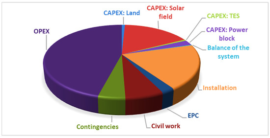
Figure 5.
Share of expenses for base case parabolic trough plant over 25 years.
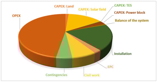
Figure 6.
Share of expenses for base case solar power tower plant over 25 years.
6. Results and Discussion
Table 10 reports the efficiencies of three electricity generation cycles considered in this study, followed by different operating temperatures and pressures that are reverent for CSP system outlay. Due to the higher temperature attainment in the SPT configuration, both the Rankine and Brayton cycles can operate at higher temperatures and pressures, resulting in higher operational efficiencies. Since the temperature attainment potential of the PT configuration is lower than that of the SPT configuration, the plants were designed to operate with medium temperature and pressure thermal cycles. In the combined cycle scenarios, the evaluation was performed based on the topping cycle, in which the Brayton cycle generates electricity first, and then the Rankine cycle is operated from the gas turbine output.
Table 10.
Operational parameters for Rankine, Brayton, and combined cycles.
The mathematical model thus developed was used to assess the LCOE variation of the TES-integrated CSP plant using the MS Excel software for the 18 scenarios considered in this study. Table 11, Table 12, Table 13 and Table 14 report the results. When comparing the simulation of the energy system under two base cases defined above, scenario 1 and scenario 13, both of which use a regular TES medium, scenario 1 shows the lowest LCOE and highest CSP plant efficiency, and this increased plant efficiency could be the reason behind the decreased LCOE. Despite the comparatively lower efficiency of the TES, the increased solar field efficiency in scenario 1 can be identified as the reason for increased CSP plant capacity. The minimum LCOE (7.72 ct/kWh) among all nine scenarios for the same installed capacity of a 50 MW plant with regular TES medium is shown by scenario 15, which consists of SPT CSP configuration along with LHTES to drive the combined cycle electricity generation. Furthermore, this scenario has the highest CSP plant overall efficiency (22.14%). This increased efficiency is due to the increased efficiency of the combined power cycle. Furthermore, it can be seen that scenario 15 has the lowest TES efficiency among scenarios that include LHTES, which uses the regular TES medium (Scenario 13, Scenario 14, and Scenario 15). Therefore, the end-use thermal cycle can contribute significantly to the round-trip efficiency of a CSP plant. This pattern can be seen in all scenarios that use the combined power cycle as opposed to the Rankine or Brayton cycles. This same reason can be attributed to the lower LCOE of scenario 15 among regular storage medium-based LHTES in SPT plant scenarios, despite the higher CAPEX and thus OPEX associated with the combined cycle. However, when scenario 15 is compared to scenarios 1–6, this pattern does not follow, most likely due to the inability of efficiency improvement to exceed the CAPEX and OPEX of the combined cycle equipment. Scenario 4 shows the lowest energy cost of 9.30 ct/kWh, while scenario 6 shows the highest CSP plant efficiency (16.01%) for the PT scenarios only. Scenario 2, with the combination of PT CSP configuration with SHTES for energy storage and end application, is the single-stage Brayton cycle that has the highest LCOE of 10.41 ct/kWh with 13.21% power plant efficiency. Scenario 13, the SPT base case, shows the minimum CSP plant efficiency (12.02%) with an LCOE of 9.81 ct/kWh in SPT-based scenarios.
Table 11.
LCOE analysis for a parabolic trough plant of 50 MW installed capacity with regular storage medium.
Table 12.
Solar power tower plant LCOE analysis for 50 MW installed capacity with regular storage medium.
Table 13.
LCOE analysis for a parabolic trough plant of 100 MW installed capacity with nano-enhanced storage medium.
Table 14.
LCOE analysis for a solar power tower plant of 100 MW installed capacity with nano-enhanced storage medium.
In all CSP and TES combinations, the combined cycle as the end-use thermal application has a lower LCOE and higher CSP plant efficiency than the single-stage Rankine and Brayton cycles. Furthermore, the use of the Rankine cycle in PT-based scenarios results in more economical energy generation with improved plant efficiencies, whereas the opposite is true in SPT-based scenarios. The use of the Brayton cycle over the Rankine cycle reduces energy system efficiency by a maximum of 1.42% while increasing LCOE by 0.11% in the PT configuration with SHTES. The use of the Brayton cycle over the Rankine cycle in the PT configuration with LHTES results in a 1.38% reduction in energy system efficiency with no significant change in LCOE. In contrast, in SPT configuration with LHTES, the use of the Brayton cycle over Rankine improves CSP plant efficiency by 37.35% while lowering energy costs by 11.82%. Overall, the LCOE appears to be inversely proportional to the efficiency of the CSP plant. Therefore, the use of the Rankine cycle can reduce energy costs at higher operating temperatures and pressures, but not at medium or low temperatures and pressures.
Furthermore, based on an industrial design consideration, this study varied the TES size based on the end-use energy requirement. As a result, the efficiency of the TES varies as the effective area of thermal loss changes. The TES efficiency appeared to be highest in Rankine cycle-based scenarios and lowest in combined cycle-based scenarios. Scenario 4 (PT plant with LHTES for Rankine cycle) has the highest TES efficiency (92.40%) of all nine scenarios. Scenario 15 (SPT with LHTES for combined cycle operation) has the lowest TES efficiency of all. Furthermore, the evaluation of TES’s contribution to CAPEX was studied, and scenario 15 shows the lowest cost of TES, while scenario 2 shows the highest contribution of TES to CAPEX. Overall, it can be seen that the SPT plant with LHTES has lower TES costs; hence, the overall performance improvement relies on solar field optimization. These findings are presented in Table 11 and Table 12, and Figure 7 and Figure 8 graphically depict the comparison of scenarios. Even further, it can be seen that LHTES in SPT plants, particularly those with the combined cycle for electricity generation, are the best candidates for future CSP plants. LHTES is a superior substitute for conventional SHTES found in PT power plants.
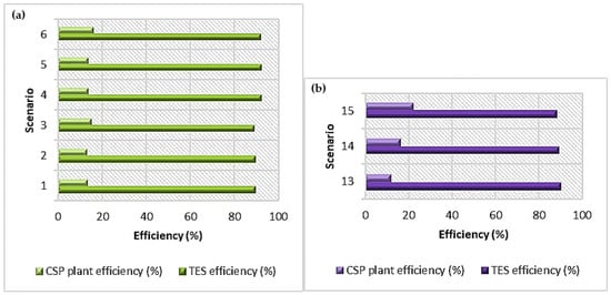
Figure 7.
CSP plant efficiency and TES efficiency of (a) PT power plants and (b) SPT power plants under regular TES medium.
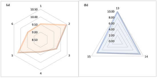
Figure 8.
LCOE of (a) PT power plants (scenario 1–6) and (b) SPT power plants (scenario 13–15) with regular TES medium.
The study also looked at how the LCOE changed as the installed capacity of CSP plants increased. Plant capacity was increased from 50 MW to 100 MW, and the results show a reduction in LCOE in all scenarios, as shown in Figure 9. This improvement follows a similar pattern. Following the same pattern, CSP plant efficiency tends to increase, with a 2.53% plant efficiency improvement seen in scenario 15, the combination that demonstrated the highest CSP plant efficiency of all scenarios mentioned. The scenario with the highest CSP plant efficiency in the PT type results in a 1.69% increase in plant efficiency. Similarly, as plant capacity increases, TES efficiency rises in all scenarios. Furthermore, as TES sizes increased to store more energy for end-use thermal applications along with the plant capacity increment, the TES cost contribution to CAPEX and OPEX increased. However, the increase in energy production as a result of the higher operational efficiencies has surpassed the cost increase as a result of the larger TES, resulting in the overall LCOE reduction mentioned above.
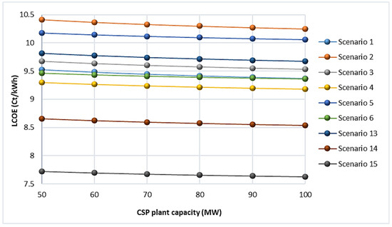
Figure 9.
LOCE reduction with CSP plant capacity increment.
Many research papers have been published, and details on improving the thermo-physical properties of TES medium by adding nanoparticles of a compatible material can be found in the open literature. Among those studies, Hamdy et al. [68], Lasfargues et al. [69], Huang et al. [70], Li et al. [71], and Chieruzzi et al. [72] show great potential in improving storage material energy density with the addition of nanoparticles. Following that, the nano-enhanced storage medium-driven CSP plants were evaluated using a hypothesis that assumes a maximum 5% increase in storage material energy density for a 10% increase in storage material cost. As 100 MW CSP plants have the lowest LCOE for the capacity range considered here, the remaining nine scenarios for nano-enhanced TES medium are being considered for 100 MWe of installed plant capacity in order to select the best-performing power plant configuration from each PT and SPT type for the further study. As a result, the LCOE, CSP plant efficiency, and TES efficiency variation were investigated. The results obtained are shown in Table 13 and Table 14. These findings are depicted graphically in Figure 10 and Figure 11. As a result, the LCOE results obtained for a 100 MW power plant after nanoparticle improvement were compared to the LCOE of each scenario using the regular TES medium for the 50 MW installed capacity. Figure 12 depicts the comparison, which shows that all plants have decreased their energy costs as the combined effect of nanoparticle integration and increment of installed plant capacity. The letter “C” denotes scenario conversions from a regular TES material-based 50 MW power plant to its identical nano-enhanced TES material-based 100 MW power plant. In this case, the C numbers 1 to 9 represent the conversion of PT scenarios 1 to 6 into scenarios 7 to 12 and the conversion of SPT scenarios 13 to 15 into scenarios 16 to 18. Among all the nano-enhancement scenarios, it is seen that the use of combined cycle results in the minimum LCOE. Following that, the transformation from scenario 1 to 7 accounts for the greatest LCOE reduction, while the transformation from scenario 5 to 11 accounts for the lowest LCOE increase, where both scenarios are based on parabolic trough plants.
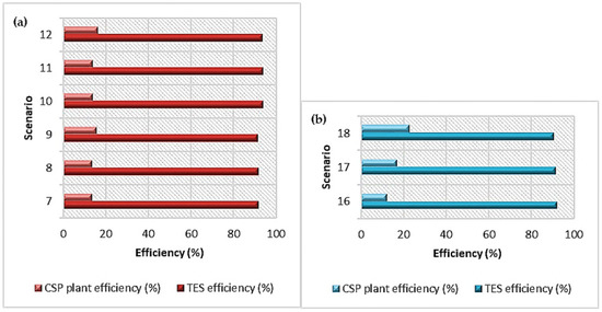
Figure 10.
CSP plant efficiency and TES efficiency of 100 MW (a) PT power plants and (b) SPT power plants under nano-enhanced TES medium.
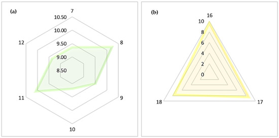
Figure 11.
LCOE of 100 MW (a) PT power plants (scenario 7–12) and (b) SPT power plants (scenario 16–18) with nano-enhanced TES medium.
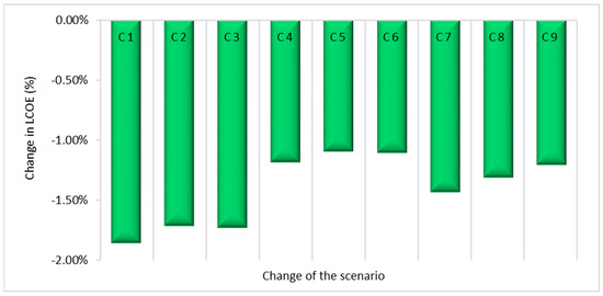
Figure 12.
LCOE variation of CSP plants with the introduction of nanoparticles and doubling the installed plant capacity. Here, C1, C2, C3, C4, C5, C6, C7, C8 and C9 represent the conversion of scenarios from 1 to 7, 2 to 8, 3 to 9, 4 to 10, 5 to 11, 6 to 12, 13 to 16, 14 to 17, and 15 to 18, respectively.
In comparison to the base case, the variations in LCOE for scenarios 2 to 12 for a 50 MW parabolic trough plant are 9.3%, 1.6%, −2.4%, 6.8%, −0.7%, 7.4%, −0.2%, −3.6%, 5.6%, and −1.8%, respectively. As a result, the overall variation exhibits mixed performance. In contrast, scenarios 14 to −18 for a 50 MW solar power tower plant show −11.8%, −21.3%, −1.4%, −13.0%, and −22.3% of an LCOE variation where all plant configurations show less energy generation cost than the base case. Based on the results, no such solid pattern can be identified to predict the LCOE variation in conjunction with the nanoparticle-based performance improvement. As a result, power plants under scenario 10 to represent parabolic trough CSP plants, and scenario 18, which represents solar power tower plants, were chosen for further study based on their lower energy cost. However, it can be seen that the cost of electricity generation can be reduced by selecting appropriate materials in combination with nanoparticle additives. As a result, the mathematical model developed in this study can be refined to determine the most effective TES-integrated CSP pant configuration.
7. Conclusions
This paper presents a mathematical model to predict the LCOE variation of TES-integrated CSP power plants for electricity generation. Parabolic trough (PT) and solar power tower (SPT) plant configurations with SHTES and LHTES with the regular storage medium and nano-enhanced storage medium were considered. Rankine cycle, Brayton cycle, and combined power generation cycle were considered for comparison. Altogether, 18 scenarios were treated under the aforementioned combinations. Nine scenarios, scenarios 1 to 6 and 13 to 15, were dedicated to investigating the variation in electricity production costs with regular storage materials. Scenarios 7 to 12 and 16 to 18 were dedicated to evaluating the LCOE variation under nano-enhanced TES materials. Two of the 18 scenarios, i.e., scenario 1, representing parabolic trough (PT), and scenario 13, representing solar power tower (SPT) configurations, were designated as base cases using the USA-based cost details to facilitate the comparison.
Calculations of LCOE, TES contribution for LCOE, CSP plant efficiency, and TES efficiency were performed using the developed mathematical model. The results showed that the LHTES was preferred over the SHTES in terms of the energy generation cost of CSP plants. Moreover, the combined power cycle can improve the overall efficiency of the CSP plant in terms of energy utilization, and LCOE reduction appears to deliver competitive results, especially in SPT plants. Noticeably, the selection of the end-use thermal cycle is heavily influenced by the temperature level that the designated CSP plant can achieve. As a result, this will directly affect the round-trip efficiency of the CSP plant and LCOE.
Furthermore, scenario 15, which consists of SPT configuration with LHTES with regular storage medium to drive combined cycle electricity generation, returned the lowest LCOE of 7.72 ct/kWh and the highest CSP plant efficiency of 22.14% among the first nine scenarios considered. The same combination, but with the storage medium replaced with nano-enhanced material for 100 MW of installed plant capacity (scenario 18), returned a 7.63 ct/kWh minimum LCOE with a 22.70% CSP plant efficiency. Therefore, the incorporation of nano additives into storage materials could improve CSP plant performance while lowering the LCOE. Based on these results, the aforementioned scenarios 18, representing SPT plants, and 10, which shows 9.19 ct/kWh of LCOE and 14.03% CSP plant efficiency, representing PT plants, were chosen for further investigation on LCOE reduction under different DNI conditions.
Work presented in this paper is limited by the PT and SPT configurations with single tank thermocline-type SHTES and LHTES. In fact, some more options are available for CSP plants, such as the thermos-chemical energy storage, two-tank configuration, shell and tube heat exchangers, and cascade TES. More work is underway to evaluate the potential of these options and will be presented in a future communication.
Author Contributions
Conceptualization, H.K.; methodology, D.J.; formal analysis, D.J.; investigation, D.J.; resources, S.W., H.K. and J.A.W.; data curation, D.J.; writing—original draft preparation, D.J.; writing—review and editing, S.W., H.K. and J.A.W.; visualization, D.J.; supervision, S.W. and H.K. All authors have read and agreed to the published version of the manuscript.
Funding
This research received no external funding.
Institutional Review Board Statement
Not applicable.
Informed Consent Statement
Not applicable.
Data Availability Statement
Not applicable.
Conflicts of Interest
The authors declare no conflict of interest.
Nomenclature
| It | Investment cost in the year t (USD) |
| Mt | Operational and Maintenance cost in the year t (USD) |
| Ft | Fuel cost in the year t (USD) |
| Et | Energy generated in year t (kWh) |
| r | Discount rate (%) |
| n | Life span of the CSP plant (years) |
| A1 | Area of solar collector one unit (m2) |
| N | Number of solar collectors needed (units) |
| DNI | Direct Normal Irradiance (kWh/m2/year) |
| A1 | Area of solar collector one unit (m2) |
| LAT | Total land area (m2) |
| PrL | Unit area price (USD) |
| CL | Cost of the land (USD) |
| CS | Cost of the solar collectors (USD) |
| PrS | Unit price of solar collector (USD) |
| CTES | TES cost (USD) |
| mSM | Storage material mass quantity (kg) |
| PrSM | Unit price of the storage medium (USD) |
| mCM | Container material mass quantity (kg) |
| PrCM | Unit price of the container material (USD) |
| CAC | Cost of auxiliary components (USD) |
| SM | Solar multiplier |
| ηcollector | Solar collector efficiency (%) |
| ηreceiver | Receiver efficiency (%) |
| ηHTF | HTF efficiency (%) |
| ηHE | Heat Exchanger efficiency (%) |
| NHE | Number of heat exchangers in the system (units) |
| ηTES | TES system efficiency (%) |
| ηthermal | Power cycle thermal efficiency (%) |
| ηT | Turbine efficiency (%) |
| ηG | Generator efficiency (%) |
| PT | Total solar power captured by the mirrors (kWh/year) |
| Ai | Solar collector area of ith collector (m2) |
| θi | Angle between the incident solar rays and normal to ith mirror element (rad) |
| fsp, i | Spillage factor |
| fat, i | Attenuation factor |
| fb | Blocking factor |
| fsh | Shadowing factor |
| αc | Reflectivity |
| foptical | Factor for optical efficiency |
| D | Distance between the solar collector and the focal point of the receiver (m) |
| qloss,receiver | Heat loss in the receiver (kJ) |
| qsolar incident | Incident Solar Power on the receiver (kJ) |
| qin,HTF | Solar power transferred to HTF (kJ) |
| qrad | Radiation heat loss (kJ) |
| qconv | Convection heat loss (kJ) |
| SF | Radiation shape factor of the receiver = 1 |
| AR | Radiative area of the receiver (m2) |
| ε | Emissivity of the receiver |
| σ | Stefan Boltzmann constant (5.67037442 × 10⁻⁸ kg s−3 K−4) |
| TR | Temperature of the receiver (K) |
| Tambient | Ambient temperature (K) |
| hconv | Convective heat transfer coefficient (kW/m2 K) |
| HR | Total height of the receiver (m) |
| ηTES | TES efficiency (%) |
| qout,HTF | Thermal energy from HTF (kJ) |
| ETES | Energy stored in the TES (kJ) |
| ηHE | Efficiency of heat exchanger (%) |
| Eloss,TES | Thermal energy loss from TES (kJ) |
| UTES | Overall heat transfer coefficient (W/m2 K) |
| Aht | Heat transfer area (m2) |
| TTES | Temperature at TES outlet (K) |
| Tambient | Ambient temperature (K) |
| H | Height of the TES (m) |
| DTES | Diameter of the TES (m) |
| ESHTES | Amount of heat energy can be stored in SHTES (kJ) |
| ELHTES | Amount of heat energy can be stored in LHTES (kJ) |
| mSHTES | Storage material mass of SHTES (kg) |
| mLHTES | Storage material mass of LHTES (kg) |
| CP | Specific heat capacity of storage medium of SHTES (Solid or Liquid) (kJ/kg K) |
| CPS | Specific heat capacity of storage medium of LHTES in solid state (kJ/kg K) |
| CPL | Specific heat capacity of storage medium of LHTES in liquid state (kJ/kg K) |
| Tmelt | Melting temperature of storage medium (K) |
| Hm | Melting enthalpy of storage medium (kJ/kg) |
| am | Melting fraction |
| Tinitial | Initial temperature of storage medium (K) |
| Tfinal | Final temperature of storage medium (K) |
| V/V0 | Melted volume fraction |
| Fo | Fourier number |
| Ste | Stephan number |
| Ra | Rayleigh number |
| CATES | TES capacity (kJ) |
| CACSP | CSP plant capacity (kJ) |
| hOP | Operational hours without the heat source (hours) |
| EDSHM | Energy density of sensible heat storage material (kJ/kg) |
| EDLHM | Energy density of latent heat storage material (kJ/kg) |
| VTES | TES tank volume (m3) |
| ρSHTES | Density of the sensible heat storage medium (kg/m3) |
| ρLHTES | Density of the latent heat storage medium (kg/m3) |
| Vstorage medium | Storage medium volume (m3) |
| Ddischarge | Discharging time of the storage (hours) |
| QHTF | Heat transfer rate of HTF (kW) |
| ṁHTF | HTF mass flow rate (kg/s) |
| CP, HTF | Specific heat capacity of the HTF (kJ/kg K) |
| Tthermal | Thermal cycle-required temperature (K) |
| ρHTF | HTF density (kg/m3) |
| Apipe | Cross-section of the HTF pipe (m2) |
| ν | HTF flow velocity (m/s) |
| ρcomposite | Density of the nanocomposite (kg/m3) |
| ρr | Density of the regular storage material (kg/m3) |
| ρn | Density of the nanomaterial (kg/m3) |
| Nanoparticle concentration (wt.%) | |
| CP,r | Specific heat capacity of the regular storage medium (kJ/kg K) |
| CP,np | Specific heat capacity of the nanomaterial (kJ/kg K) |
| CP,composite | Specific heat capacity of the nanocomposite (kJ/kg K) |
| ηR | Efficiency of the Rankine cycle (%) |
| ηB | Efficiency of the Brayton cycle (%) |
| ∆H1 | Enthalpy variation of steam at condenser heat rejection (kJ/kg) |
| ∆H2 | Enthalpy variation of steam at heat intake (kJ/kg) |
| qin | Thermal energy from TES (kWh) |
| Wout | Work output from the turbine (kWh) |
| Win | Work input by pumps (kWh) |
| rp | Pressure ratio of air |
| k | Specific heat ratio of air |
| ηCC | Efficiency of the combined cycle (%) |
| CF | Capacity factor |
| Eelec, actual | Actual electricity production per year (kWh) |
| Eelec, theoretical | Theoretical maximum electricity production per year (kWh) |
| Esolar | Solar energy received to the CSP plant for a year (kWh) |
References
- Modi, A.; Bühler, F.; Andreasen, J.G.; Haglind, F. A review of solar energy based heat and power generation systems. Renew. Sustain. Energy Rev. 2017, 67, 1047–1064. [Google Scholar] [CrossRef]
- Jouhara, H.; Żabnieńska-Góra, A.; Khordehgah, N.; Ahmad, D.; Lipinski, T. Latent thermal energy storage technologies and applications: A review. Int. J. Thermofluids 2020, 5–6, 100039. [Google Scholar] [CrossRef]
- Achkari, O.; El Fadar, A. Latest developments on TES and CSP technologies—Energy and environmental issues, applications and research trends. Appl. Therm. Eng. 2020, 167, 114806. [Google Scholar] [CrossRef]
- Richter, C. Concentrating Solar Power Global Outlook. 2009. Available online: http://scholar.google.com/scholar?hl=en&btnG=Search&q=intitle:Concentrating+Solar+Power+Global+Outlook+09#0 (accessed on 23 August 2022).
- Müller-Steinhagen, H.; Trieb, F. Concentrating solar power—A review of the technology. Ingenia 2004, 18, 43–50. [Google Scholar]
- Boretti, A.; Castelletto, S.; Al-Zubaidy, S. Concentrating solar power tower technology: Present status and outlook. Nonlinear Eng. 2019, 8, 10–31. [Google Scholar] [CrossRef]
- Nallusamy, N.; Sampath, S.; Velraj, R. Experimental investigation on a combined sensible and latent heat storage system integrated with constant/varying (solar) heat sources. Renew. Energy 2007, 32, 1206–1227. [Google Scholar] [CrossRef]
- Kumar, A.; Shukla, S. A Review on Thermal Energy Storage Unit for Solar Thermal Power Plant Application. Energy Procedia 2015, 74, 462–469. [Google Scholar] [CrossRef]
- Jawhar, N.S.; Witharana, S.; Nggada, S.; Talib, A.; Belachew, C.; Li, Y. Thermal Energy Storage Options for Concentrated Solar Power Plants in the United Arab Emirates. In Proceedings of the 2020 Advances in Science and Engineering Technology International Conferences (ASET), Dubai, United Arab Emirates, 4 February–9 April 2020. [Google Scholar] [CrossRef]
- Thakare, K.A.; Bhave, A.G. Review on Latent Heat Storage and Problems Associated with Phase Change Materials. Int. J. Res. Eng. Technol. 2015, 4, 176–182. [Google Scholar] [CrossRef]
- Khan, Z.; Khan, Z.; Ghafoor, A. A review of performance enhancement of PCM based latent heat storage system within the context of materials, thermal stability and compatibility. Energy Convers. Manag. 2016, 115, 132–158. [Google Scholar] [CrossRef]
- Gasa, G.; Lopez-roman, A.; Prieto, C.; Cabeza, L.F. Life cycle assessment of a concentrating solar power plant in tower configuration with and without thermal energy storage. Sustainability 2021, 13, 3672. [Google Scholar] [CrossRef]
- Yang, L.; Huang, J.-N.; Zhou, F. Thermophysical properties and applications of nano-enhanced PCMs: An update review. Energy Convers. Manag. 2020, 214, 112876. [Google Scholar] [CrossRef]
- Liu, M.; Saman, W.; Bruno, F. Review on storage materials and thermal performance enhancement techniques for high temperature phase change thermal storage systems. Renew. Sustain. Energy Rev. 2012, 16, 2118–2132. [Google Scholar] [CrossRef]
- Sharma, A.; Tyagi, V.V.; Chen, C.R.; Buddhi, D. Review on thermal energy storage with phase change materials and applications. Renew. Sustain. Energy Rev. 2009, 13, 318–345. [Google Scholar] [CrossRef]
- Enescu, D.; Chicco, G.; Porumb, R.; Seritan, G. Thermal Energy Storage for Grid Applications: Current Status and Emerging Trends. Energies 2020, 13, 340. [Google Scholar] [CrossRef]
- Lin, Y.; Jia, Y.; Alva, G.; Fang, G. Review on thermal conductivity enhancement, thermal properties and applications of phase change materials in thermal energy storage. Renew. Sustain. Energy Rev. 2018, 82, 2730–2742. [Google Scholar] [CrossRef]
- Dash, L.; Mahanwar, P.A. A review on organic phase change materials and their applications. Int. J. Eng. Appl. Sci. Technol. 2021, 5, 268–284. [Google Scholar] [CrossRef]
- Lin, Y.; Alva, G.; Fang, G. Review on thermal performances and applications of thermal energy storage systems with inorganic phase change materials. Energy 2018, 165, 685–708. [Google Scholar] [CrossRef]
- Gil, A.; Medrano, M.; Martorell, I.; Lázaro, A.; Dolado, P.; Zalba, B.; Cabeza, L.F. State of the art on high temperature thermal energy storage for power generation. Part 1—Concepts, materials and modellization. Renew. Sustain. Energy Rev. 2010, 14, 31–55. [Google Scholar] [CrossRef]
- Dowling, A.W.; Zheng, T.; Zavala, V.M. Economic assessment of concentrated solar power technologies: A review. Renew. Sustain. Energy Rev. 2017, 72, 1019–1032. [Google Scholar] [CrossRef]
- Trieb, F.; Schillings, C.; Sullivan, M.; Pregger, T.; Hoyer-klick, C. Global Potential of Concentrating Solar Power. 2009, pp. 1–11. Available online: http://www.dlr.de/tt/en/Portaldata/41/Resources/dokumente/institut/system/projects/reaccess/DNI-Atlas-SP-Berlin_20090915-04-Final-Colour.pdf (accessed on 22 June 2022).
- IRNEA. Renewable Power Generation Costs in 2020. Available online: https://www.irena.org/-/media/Files/IRENA/Agency/Publication/2018/Jan/IRENA_2017_Power_Costs_2018.pdf (accessed on 5 May 2022).
- Aseri, T.K.; Sharma, C.; Kandpal, T.C. Estimation of capital costs and techno-economic appraisal of parabolic trough solar collector and solar power tower based CSP plants in India for different condenser cooling options. Renew. Energy 2021, 178, 344–362. [Google Scholar] [CrossRef]
- Musi, R.; Grange, B.; Sgouridis, S.; Guedez, R.; Armstrong, P.; Slocum, A.; Calvet, N. Techno-economic analysis of concentrated solar power plants in terms of levelized cost of electricity. AIP Conf. Proc. 2017, 1850, 160018. [Google Scholar] [CrossRef]
- Mahlangu, N.; Thopil, G.A. Life cycle analysis of external costs of a parabolic trough Concentrated Solar Power plant. J. Clean. Prod. 2018, 195, 32–43. [Google Scholar] [CrossRef]
- Hussain, C.M.I.; Muppala, S.; Chowdhury, N.; Adnan, A. Cost analysis of concentrated solar power plant with thermal energy storage system in Bangladesh. Int. J. Enhanc. Res. Sci. Technol. Eng. 2013, 2, 79–87. [Google Scholar]
- Concentrated Solar Power’ Images|Adobe Stock. 2022. Available online: https://stock.adobe.com/fr/search?k=%22concentrated+solar+power%22&continue-checkout=1&asset_id=303721938 (accessed on 22 November 2022).
- Zarma, I.H.; Hassan, H.; Ookawara, S.; Ahmed, M. Thermal Energy Storage in Phase Change Materials—Applications, Advantages and Disadvantages. In Proceedings of the 1st International Conference of Chemical, Energy and Environmental Engineering, Alexandria, Egpyt, 19–21 March 2017. [Google Scholar]
- Cabeza, L.F.; Galindo, E.; Prieto, C.; Barreneche, C.; Fernández, A.I. Key performance indicators in thermal energy storage: Survey and assessment. Renew. Energy 2015, 83, 820–827. [Google Scholar] [CrossRef]
- Karunathilake, H.; Hewage, K.; Brinkerhoff, J.; Sadiq, R. Optimal renewable energy supply choices for net-zero ready buildings: A life cycle thinking approach under uncertainty. Energy Build. 2019, 201, 70–89. [Google Scholar] [CrossRef]
- García-Ferrero, J.; Merchán, R.; Santos, M.; Medina, A.; Hernández, A.C. Brayton technology for Concentrated Solar Power plants: Comparative analysis of central tower plants and parabolic dish farms. Energy Convers. Manag. 2022, 271, 116312. [Google Scholar] [CrossRef]
- Corona, B.; Cerrajero, E.; López, D.; Miguel, G.S. Full environmental life cycle cost analysis of concentrating solar power technology: Contribution of externalities to overall energy costs. Sol. Energy 2016, 135, 758–768. [Google Scholar] [CrossRef]
- Pelay, U.; Azzaro-Pantel, C.; Fan, Y.; Luo, L. Life cycle assessment of thermochemical energy storage integration concepts for a concentrating solar power plant. Environ. Prog. Sustain. Energy 2020, 39, e13388. [Google Scholar] [CrossRef]
- Turchi, C.S.; Boyd, M.; Kesseli, D.; Kurup, P.; Mehos, M.; Neises, T.; Sharan, P.; Wagner, M.J.; Wendelin, T. CSP Systems Analysis—Final Project Report. Nrel/TP-5500-72856. 2019. Available online: www.nrel.gov/publications (accessed on 11 November 2022).
- Dieckmann, S.; Dersch, J.; Giuliano, S.; Puppe, M.; Lüpfert, E.; Hennecke, K.; Pitz-Paal, R.; Taylor, M.; Ralon, P. LCOE reduction potential of parabolic trough and solar tower CSP technology until 2025. AIP Conf. Proc. 2017, 1850, 160004. [Google Scholar] [CrossRef]
- Behar, O.; Sbarbaro, D.; Morán, L. A Practical Methodology for the Design and Cost Estimation of Solar Tower Power Plants. Sustainability 2020, 12, 8708. [Google Scholar] [CrossRef]
- Shagdar, E.; Lougou, B.G.; Sereeter, B.; Shuai, Y.; Mustafa, A.; Ganbold, E.; Han, D. Performance Analysis of the 50 MW Concentrating Solar Power Plant under Various Operation Conditions. Energies 2022, 15, 1367. [Google Scholar] [CrossRef]
- Yang, J.; Yang, Z.; Duan, Y. Novel design optimization of concentrated solar power plant with S-CO2 Brayton cycle based on annual off-design performance. Appl. Therm. Eng. 2021, 192, 116924. [Google Scholar] [CrossRef]
- How Much Does Land Cost in the United States? Available online: https://discountlots.com/how-much-does-land-cost-in-the-us/ (accessed on 14 November 2022).
- Liu, M.; Tay, N.S.; Bell, S.; Belusko, M.; Jacob, R.; Will, G.; Saman, W.; Bruno, F. Review on concentrating solar power plants and new developments in high temperature thermal energy storage technologies. Renew. Sustain. Energy Rev. 2016, 53, 1411–1432. [Google Scholar] [CrossRef]
- Layton, A.; Reap, J.; Bras, B.; Weissburg, M. Correlation between Thermodynamic Efficiency and Ecological Cyclicity for Thermodynamic Power Cycles. PLoS ONE 2012, 7, e51841. [Google Scholar] [CrossRef] [PubMed]
- Trevisan, S.; Ruan, T.; Wang, W.; Laumert, B. Techno-economic analysis of an innovative purely solar driven combined cycle system based on packed bed TES technology. AIP Conf. Proc. 2020, 2303, 130008. [Google Scholar] [CrossRef]
- Caraballo, A.; Galán-Casado, S.; Caballero, Á.; Serena, S. Molten Salts for Sensible Thermal Energy Storage: A Review and an Energy Performance Analysis. Energies 2021, 14, 1197. [Google Scholar] [CrossRef]
- PlusICE. PlusICE Range. 2018. Available online: www.pcmproducts.net (accessed on 25 March 2022).
- Ahmed, N.; Elfeky, K.; Lu, L.; Wang, Q. Thermal and economic evaluation of thermocline combined sensible-latent heat thermal energy storage system for medium temperature applications. Energy Convers. Manag. 2019, 189, 14–23. [Google Scholar] [CrossRef]
- Merchán, R.; Santos, M.; García-Ferrero, J.; Medina, A.; Hernández, A.C. Thermo-economic and sensitivity analysis of a central tower hybrid Brayton solar power plant. Appl. Therm. Eng. 2020, 186, 116454. [Google Scholar] [CrossRef]
- Dunham, M.T.; Iverson, B.D. High-efficiency thermodynamic power cycles for concentrated solar power systems. Renew. Sustain. Energy Rev. 2014, 30, 758–770. [Google Scholar] [CrossRef]
- Giaconia, A.; Iaquaniello, G.; Metwally, A.A.; Caputo, G.; Balog, I. Experimental demonstration and analysis of a CSP plant with molten salt heat transfer fluid in parabolic troughs. Sol. Energy 2020, 211, 622–632. [Google Scholar] [CrossRef]
- Pang, L.; Wang, T.; Li, R.; Yang, Y. Two-stage solar power tower cavity-receiver design and thermal performance analysis. AIP Conf. Proc. 2017, 1850, 30037. [Google Scholar] [CrossRef]
- Talebizadeh, P.; Mehrabian, M.A.; Rahimzadeh, H. Optimization of Heliostat Layout in Central Receiver Solar Power Plants. J. Energy Eng. 2014, 140, 04014005. [Google Scholar] [CrossRef]
- Hussaini, Z.A.; King, P.; Sansom, C. Numerical Simulation and Design of Multi-Tower Concentrated Solar Power Fields. Sustainability 2020, 12, 2402. [Google Scholar] [CrossRef]
- Atif, M.; Al-Sulaiman, F.A. Energy and Exergy Analyses of Recompression Brayton Cycles Integrated with a Solar Power Tower through a Two-Tank Thermal Storage System. J. Energy Eng. 2018, 144, 04018036. [Google Scholar] [CrossRef]
- Ma, Z.; Glatzmaier, G.; Turchi, C.; Wagner, M. Thermal energy storage performance metrics and use in thermal energy storage design. In Proceedings of the ASES World Renewable Energy Forum, Denver, CO, USA, 13–17 May 2012; pp. 1054–1059. [Google Scholar]
- Jayathunga, D.; Karunathilake, H.; Narayana, M.; Witharana, S. Selection of phase change materials for high temperature latent heat thermal energy storage for concentrated solar power plants. In Proceedings of the 2022 Moratuwa Engineering Research Conference (MERCon), Moratuwa, Sri Lanka, 27–29 July 2022. [Google Scholar] [CrossRef]
- Vilella, A.G.; Yesilyurt, S. Analysis of Heat Storage with a Thermocline Tank for Concentrated Solar Plants: Application to AndaSol I. In Proceedings of the 2015 International Conference on Industrial Technology (ICIT), Seville, Spain, 17–19 March 2015; pp. 2750–2755. [Google Scholar] [CrossRef]
- Sarbu, I.; Dorca, A. Review on heat transfer analysis in thermal energy storage using latent heat storage systems and phase change materials. Int. J. Energy Res. 2018, 43, 29–64. [Google Scholar] [CrossRef]
- Ho, C.; Gao, J. Preparation and thermophysical properties of nanoparticle-in-paraffin emulsion as phase change material. Int. Commun. Heat Mass Transf. 2009, 36, 467–470. [Google Scholar] [CrossRef]
- Khodadadi, J.M.; Fan, L. Expedited Freezing of Nanoparticle-Enhanced Phase Change Materials (NEPCM) Exhibited Through a Simple 1-D Stefan Problem Formulation. In Proceedings of the ASME 2009 Heat Transfer Summer Conference collocated with the InterPACK09 and 3rd Energy Sustainability Conferences, San Francisco, CA, USA, 19–23 July 2009; pp. 345–351. [Google Scholar] [CrossRef]
- Yu, Y.; Zhao, C.; Tao, Y.; Chen, X.; He, Y.-L. Superior thermal energy storage performance of NaCl-SWCNT composite phase change materials: A molecular dynamics approach. Appl. Energy 2021, 290, 116799. [Google Scholar] [CrossRef]
- Dudda, B.; Shin, D. Effect of nanoparticle dispersion on specific heat capacity of a binary nitrate salt eutectic for concentrated solar power applications. Int. J. Therm. Sci. 2013, 69, 37–42. [Google Scholar] [CrossRef]
- Hu, Y.; He, Y.; Zhang, Z.; Wen, D. Effect of Al2O3 nanoparticle dispersion on the specific heat capacity of a eutectic binary nitrate salt for solar power applications. Energy Convers. Manag. 2017, 142, 366–373. [Google Scholar] [CrossRef]
- Liu, M.; Severino, J.; Bruno, F.; Majewski, P. Experimental investigation of specific heat capacity improvement of a binary nitrate salt by addition of nanoparticles/microparticles. J. Energy Storage 2019, 22, 137–143. [Google Scholar] [CrossRef]
- Pincemin, S.; Olives, R.; Py, X.; Christ, M. Highly conductive composites made of phase change materials and graphite for thermal storage. Sol. Energy Mater. Sol. Cells 2008, 92, 603–613. [Google Scholar] [CrossRef]
- Kenisarin, M.; Mahkamov, K. Solar energy storage using phase change materials. Renew. Sustain. Energy Rev. 2007, 11, 1913–1965. [Google Scholar] [CrossRef]
- Kincaid, N.; Mungas, G.; Kramer, N.; Wagner, M.; Zhu, G. An optical performance comparison of three concentrating solar power collector designs in linear Fresnel, parabolic trough, and central receiver. Appl. Energy 2018, 231, 1109–1121. [Google Scholar] [CrossRef]
- Khan, M.I.; Asfand, F.; Al-Ghamdi, S.G. Progress in research and technological advancements of thermal energy storage systems for concentrated solar power. J. Energy Storage 2022, 55, 105860. [Google Scholar] [CrossRef]
- Hamdy, E.; Ebrahim, S.; Abulfotuh, F.; Soliman, M. Effect of multi-walled carbon nanotubes on thermal properties of nitrate molten salts. In Proceedings of the 2016 International Renewable and Sustainable Energy Conference (IRSEC), Marrakech, Morocco, 14–17 November 2016; pp. 317–320. [Google Scholar] [CrossRef]
- Lasfargues, M.; Geng, Q.; Cao, H.; Ding, Y. Mechanical Dispersion of Nanoparticles and Its Effect on the Specific Heat Capacity of Impure Binary Nitrate Salt Mixtures. Nanomaterials 2015, 5, 1136–1146. [Google Scholar] [CrossRef]
- Huang, Y.; Cheng, X.; Li, Y.; Yu, G.; Xu, K.; Li, G. Effect of in-situ synthesized nano-MgO on thermal properties of NaNO3-KNO3. Sol. Energy 2018, 160, 208–215. [Google Scholar] [CrossRef]
- Li, Y.; Chen, X.; Wu, Y.; Lu, Y.; Zhi, R.; Wang, X.; Ma, C. Experimental study on the effect of SiO2 nanoparticle dispersion on the thermophysical properties of binary nitrate molten salt. Sol. Energy 2019, 183, 776–781. [Google Scholar] [CrossRef]
- Chieruzzi, M.; Miliozzi, A.; Crescenzi, T.; Torre, L.; Kenny, J.M. A New Phase Change Material Based on Potassium Nitrate with Silica and Alumina Nanoparticles for Thermal Energy Storage. Nanoscale Res. Lett. 2015, 10, 273. [Google Scholar] [CrossRef]
Disclaimer/Publisher’s Note: The statements, opinions and data contained in all publications are solely those of the individual author(s) and contributor(s) and not of MDPI and/or the editor(s). MDPI and/or the editor(s) disclaim responsibility for any injury to people or property resulting from any ideas, methods, instructions or products referred to in the content. |
© 2023 by the authors. Licensee MDPI, Basel, Switzerland. This article is an open access article distributed under the terms and conditions of the Creative Commons Attribution (CC BY) license (https://creativecommons.org/licenses/by/4.0/).