Abstract
Wind and solar renewable energy in the United States is projected to triple by 2050 to nearly 30% of total electric energy generation. The upper Midwest region (Iowa, Minnesota, and North and South Dakota in particular) is considered wind energy country and not historically known for solar energy development. In this work, Value of Solar (VOS) is developed as a photovoltaic (PV) optimization measure and analysis tool using a northwest Iowa municipality as a representative case study. By applying a top-down load duration curve system analysis, VOS is used to optimize PV orientation and compare electric rate structures for increasing levels of total PV energy contribution. VOS of a fixed south-southwest orientation exceeds the levelized annual costs of installation with a larger net benefit than a one-axis-tracking solar system. Production-data modeled VOS is up to 12% higher than Typical Meteorological Year (TMY) predictions, indicating significant correlation between PV generation and peak municipal demand. Compared to alternative time-of-use rates, a demand/energy rate structure better matches VOS economic value and optimal orientation. This VOS methodology is an easy-to-use yet meaningful tool for municipalities and smaller utilities to evaluate strategic installation of and investment in PV for their local community.
1. Introduction
In the last 30 years, wind and solar renewable energy systems (RES) have grown from a negligible electric generation contribution to just over 9% of U.S. electric generation [1]. In the next 30 years, wind and solar combined are projected to triple in terms of total electricity sector contribution [2], with RES expected to represent nearly 30% of generation. From a grid stability and reliability perspective, broad studies of the Eastern [3] and Western [4] electrical interconnections of the U.S. have concluded that such levels of renewable energy penetration can be integrated without extensive infrastructure changes and would additionally be accompanied by a 25–45% reduction in carbon emissions [5].
Beyond the technical integration details and known environmental benefits, an important consideration for the increasing penetration of RES is the economic cost of integrating RES into the grid. While costs that arise from different physical impacts overlap, it is helpful for understanding to divide these integration costs into three main categories that reflect three specific characteristics of RES: (1) balancing costs due to uncertainty and unpredictability, (2) profile costs due to variability in generation, and (3) grid costs due to location specificity [6].
The first of these costs, balancing costs, are mainly operating reserves, which are typically less for solar than wind because the sun is more predictable [7]. The Western Wind and Solar Integration Study (WWSIS) reports that in the 30% renewable energy penetration case, the average variability reserve requirement does indeed double. However, with wind and solar on the system, it is often more economically favorable to back down thermal units rather than decommit them [5]. More specifically, the study noted nearly a 1:1 correlation between increased solar production and reduced combined cycle production [8]. This results in increased up-reserves being available without additional capital costs.
In regards to the third type of costs, grid costs, a recent systematic review noted that while specific data are limited, solar grid costs are typically much less than wind since solar is often installed closer to its need [7]. Heptonstall and Gross [7] further concluded that upgrades to transmission and distribution networks are difficult to allocate specifically to RES variability.
Profile costs thus emerge as the largest and most significant integration costs. These costs are linked to the temporal variability of RES with an uncontrollable output not necessarily correlated to demand [6]. Factors contributing to these costs are low RES capacity factors, and increased ramping and reduced load factors for conventional generation. While it has been shown that the direct economic impact of cycling is small, the largest single factor of integration costs is the resulting reduced utilization of capital embodied in thermal plants [6]. From a mixed cost/benefit perspective, these profile costs can be regarded as reducing the value of RES energy because they reflect diminishing avoided costs of conventional generation [6]. A methodology used to measure this changing value of PV added to the grid is Value of Solar (VOS) [9].
VOS follows a methodology more broadly defined for all distributed generation renewable energy resources called Value of Resource (VOR) [10]. VOS is VOR applied specifically to solar resources and was initially developed as a rate design mechanism intended to measure the true value of solar-PV-generated electricity. While there are ample data available on fuel and wholesale retail electricity costs [11,12], there is a lack of consensus on what renewable energy is worth. Beyond the obvious benefit of fossil fuel saved, VOS also considers avoided capacity, transmission and distribution cost deferral, and environmental benefits [9,13]. Past VOS studies have been leveraged to define a consumer energy rate for RES generation somewhere between the extremes of net-metering and displaced fuel costs [9,10,14,15,16,17]. VOS has also been analyzed for utility scale PV for 10,000 U.S. locations from 2010 to 2017 using historical nodal electricity prices, capacity market prices, marginal power system emissions, and Typical Meteorological Year (TMY) weather data to classify the value of PV in terms of displaced energy, capacity, public health, and climate change [18]. It is noted that this VOS data tends to be clustered in the Northeast, West (particularly California), and Texas. There is a notable lack of data in the upper Midwest region.
The upper Midwest (Iowa, Minnesota, and North and South Dakota in particular) is considered wind energy country and is not historically known for solar energy development. However, recent analysis suggests that a mix of solar and wind additions would be more beneficial going forward [19] and that wind and PV energy can complement one another in daily and seasonal trends [20]. Where there is a strong correlation between PV output and summer daytime peaks, adding solar PV can help make the system more reliable and/or reduce the cost of meeting peak demand [7], such that integration costs can even be negative at low (<10%) RES penetration [6].
Characterizing RES integration costs as additional expenses to be added to system generation costs has been described as a bottom-up engineering view of power system operation [7]. This work seeks to take a top-down engineering view of power system operation by analyzing the system load duration curve (LDC) before and after renewable contribution (residual LDC or RLDC) to characterize RES in terms of the value it adds to the system. A case-study is conducted for Sioux Center Municipal Utilities (SCMU) in northwest Iowa, which services more than 2700 electric customers, including a mix of residential, commercial, and industrial sites. In this way, this local analysis of SCMU can be representative of the larger upper Midwest geographical area. This work seeks to leverage the broad system considerations encompassed in VOS methodology to advance VOS as a system design benchmark and optimization tool.
PV optimization studies have been performed before. A non-constrained nonlinear optimization (‘fminsearch’ function in MATLAB [21]) was used to find the local maximum global hourly irradiation as a function of panel tilt and azimuth for locations across the continental U.S. Mapped results indicate an approximate optimum tilt of 37° from horizontal and azimuth 2° west of South (182°) for the geography of Northwest Iowa [22]. Noting that higher summer electricity prices tend to drive azimuth west and tilt towards the horizontal, a subsequent study compared the PV energy peak to market value peak using TMY weather, inverter modelling, and time-of-use rates throughout the continental U.S. as a proxy for average local grid conditions [23]. Energetically, the optimal azimuth was consistently within 10° of South for 90% of 1020 locations, while the max value of energy was found to shift more than 10° west of South for nearly half of the locations. The TMY data max energy and value azimuths for northwest Iowa both remained within 10° of South, meaning the analysis did not find an economic incentive to significantly reorient the PV array.
The focus of this work is to develop VOS as an optimization measure and analysis tool used to calculate specific VOS for the upper Midwest based on real PV production data. By applying a top-down load duration curve (LDC) system analysis, integration costs are defined from a value perspective that captures the changing value as PV contribution increases on the grid. Defining VOS in this way allows for PV system design optimization, as well as a benchmark against which different electric rate structures can be analyzed and compared. The methodology applied is considerably simpler than a full capacity-expansion system model [24], yet it provides key insights and trends consistent with findings from such studies [3,4,25,26]. As presented, this VOS methodology is an easy-to-use yet meaningful tool for municipalities and smaller utilities to evaluate investment in and guide design of PV in their local community.
2. Materials and Methods
This work uses VOS methodology to optimize system design at varying levels of PV energy contribution for Sioux Center Municipal Utilities (SCMU) in northwest Iowa, USA. The PV system is optimized for orientation: azimuth angle (East = 90°, South = 180°, West = 270°) and tilt (0° = horizontal, 90° = vertical) based on VOS modeled from real production data. PV generation is modeled from the local PV production data of a south-facing system comprised of four different tilt angles. The production data model is calibrated with generation data from three of the four tilt angles and validated against the fourth to quantify model uncertainty. Model uncertainty is propagated using Monte Carlo methods to demonstrate statistical confidence in the optimal cost savings advantage.
PV system contribution is modeled at marginal (0.1%), low (4%), medium (10%), and high (25%) levels as measured in terms of total energy generation for a nominal south-facing 41° tilt PV installation. The low value of 4% was chosen to match the current SCMU wind energy proportion [27], as well as the baseline value of the WWSIS as given by the Transmission Expansion Planning Policy Committee [26]. The high value of 25% was chosen to match the high solar case of the WWSIS [25]. The medium value of 10% was selected as a reasonable middle value and previously identified as a contribution level above which solar generation can result in overproduction [28].
2.1. Value of Solar (VOS)
VOS is calculated as the sum of net cost benefits in five major categories [9] utilizing several calculation methods [13] as outlined in Table 1. The result is presented as seven separate components which sum to give the full VOS cost savings benefit: fuel, variable operations and maintenance (VOM), capacity credit, fixed operations and maintenance (FOM), transmission and distribution (T&D), losses, and environmental (CO2). VOS is presented as energy-normalized ($/kWh) or capacity-normalized (annual $/kW).

Table 1.
Value of Solar (VOS) categories characterized as the sum of net benefits in five major categories and listed alongside the calculation method employed for seven components of net benefits in this study.
Fuel and VOM savings are calculated based on the assumption of natural gas combined cycle (CC) power plants for base and intermediate load and natural gas combustion turbine (CT) power plants for peak power using nominal performance data from the EIA Annual Outlook [11] and natural gas prices averaged over the five-year period of the study [2]. This is considered a conservative calculation given that existing power plants may operate at lower plant efficiency and different fuels (i.e., coal) compared to new CC and CT natural gas designs. Capacity credit and FOM cost savings are calculated using the overnight build and operating costs for new plants [11], while T&D savings are a combination of avoided fixed transmission costs for new plants as well as variable maintenance costs on existing infrastructure [29]. Avoided energy losses for local PV generation source versus a remote generator are calculated as a 7% multiplier on all PV generated energy [9]. Environmental cost savings are calculated from typical emissions for CC and CT power plants [30,31] and a published 39 $/ton social cost of carbon value [32] corresponding to the time frame of the PV production data.
2.2. Load Characterization
Municipal electric load is characterized using a Load Duration Curve (LDC), which plots energy demand in descending order versus relative duration. An LDC plot can be made both before and after the impact of the PV system is determined, with the after plot being called a Residual LDC (RLDC). The LDC and RLDC plots are used to characterize the electric load in terms of peak, intermediate, and base capacities based on a 15–60% division of relative duration [33]. A capacity factor (CF) is calculated for each load range, which is used in calculating levelized cost of energy (LCOE) for each type of conventional generation using methods outlined in the 2.5 Financial Analysis section. A sample LDC and RLDC plot is shown in Figure 1, including an overlay of the base, intermediate, and peak load determination for the LDC. Also included on the plot are the three major changes from the baseline LDC to a PV RLDC: (1) a peak capacity credit (peak load power is reduced), (2) a reduction in CF most noticeable in the base load, and (3) a potential for overproduction as the PV system capacity is increased [28]. The RLDC curves on the plot are generated from PV production data of a south-facing 41° tilt system.
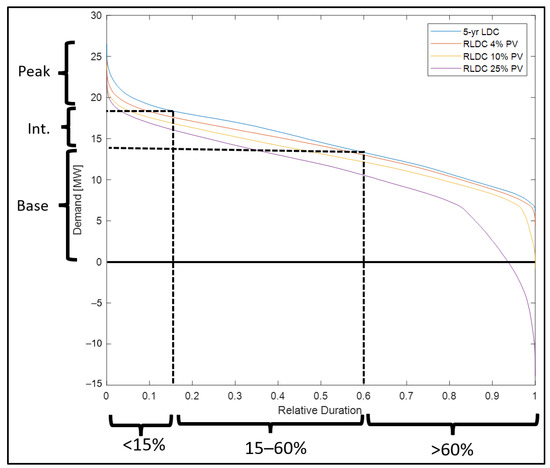
Figure 1.
Load Duration Curve (LDC) and Residual LDC (RLDC) curves illustrating peak/intermediate/base load determination based on 15–60% relative durations. RLDC plots with solar contribution show the resulting capacity credit, reduced capacity factor (CF), and overproduction impacts of increasing PV energy contribution.
2.3. PV Optimization and Uncertainty
PV generation is modelled based on local production data from a PV system within the SCMU geographical boundary. This system features south-facing panels at four different tilts (16, 29, 41, and 65° from horizontal), allowing differences in production to calibrate a beam and diffuse irradiance and system efficiency model for predicting alternative system orientation performance. This production data model uses an anisotropic sky radiation model [34], the same model used by NREL in PVWatts [35]. Data from three tilts (16, 41, and 65°) are used to calibrate and verify the model, which is validated against the 29° tilt data. Calibrated irradiance and efficiency model data are used to optimize panel tilt and azimuth for maximum VOS or annual cost savings for a particular electric rate structure.
A system model diagram of the optimization is included in Figure A1. Error associated with the model is quantified in terms of the root mean square error (RMSE) and standard deviation. The standard deviation is used in a Monte Carlo analysis to generate statistical 90% confidence intervals for the uncertainty of the modeled VOS and annual cost savings. Monte Carlo simulations of 100, 200, 400, and 800 runs are conducted to demonstrate convergence of the confidence interval uncertainty.
The PV system optimization model is also run with Typical Meteorological Year (TMY) irradiance and system efficiency data available through PVWatts [36]. Production data model results are compared to TMY to examine differences in VOS, annual cost savings, and optimal fixed system orientation. PVWatts default fixed open rack mounting PV parameters (module type, DC to AC ratio, inverter efficiency, ground coverage ratio) are assumed for TMY data, with DC losses adjusted to equalize annual production data and TMY as shown in Table A1.
2.4. Alternate Rate Structures
VOS-optimized results are compared to a second PV design optimization to maximize annual cost savings for various electric rate structures for SCMU. The existing demand/energy (D/E) price structure is outlined in Table 2. The demand listed in the table is a combination of demand and transmission charges, both of which are proportional to the peak energy demand of the month. The demand rate is seasonal, being highest in the summer, lowest in the spring and fall, and in between for winter months. The energy charge per kWh stays the same throughout the year.
Table 2.
Existing demand/energy rate structure for Sioux Center Municipal Utilities.
By examining the seasonal, monthly, weekly, and daily trends of SCMU electrical demand, alternate Time-of-Use (TOU) and Rate-of-Use (ROU) structures are designed for comparing PV cost savings to the D/E rate structure and VOS benchmark. Since a switch to TOU rates is being considered for SCMU, two TOU rate structures were designed to be applied from May to October. A midday rate (TOUm) has a peak rate applied weekdays from noon to 6:00 p.m. local time, and an intermediate rate from 7:00 a.m. to noon and 6:00 p.m. to 9:00 p.m. An evening rate (TOUe) has a peak rate applied from 3:00 p.m. to 9:00 p.m. The ROU structure is set by power demand, with peak and intermediate levels determined from the municipal LDC. The intermediate and peak rates feature a multiplier of the base rate ($/kWh), which is calculated to generate equivalent revenue for the period of analysis.
2.5. Financial Analysis
Financial calculations and analyses are consistent with methods outlined and exemplified in NREL’s Annual Technology Baseline [37]. Levelized annual cost (LAC) is used to determine annual cost savings associated with the capacity credit of the PV system. LAC is defined in Equations (1) through (3).
LCOE is Levelized Cost of Energy, FCR is Fixed Charge Rate, CAPEX is Capital Expenditures, FOM is Fixed Operations and Maintenance, CF is Capacity Factor, VOM is Variable Operations and Maintenance, and LAC is Levelized annual Cost. FCR on capital investment is calculated using the economic assumptions and parameters outlined in Table 3.
Table 3.
Economic analysis inputs, assumptions, and calculated rates following the model of NREL’s annual technology baseline [37]. The Weighted Average Cost of Capital (WACC) is the discount rate used in the net present value analysis. Inflation is the difference between nominal and real rates (nominal includes inflation). The fixed charge rate (FCR) is used in calculating the value of PV capacity credit in the annual savings, and depreciation is calculated with a 5-year Modified Accelerated Cost Recovery System (MACRS) model.
PV installation is investigated as a financial investment for SCMU using the existing D/E rate structure. The analysis is performed two different ways: simple payback and zero net present value (NPV). For simple payback, the total PV system cost is divided by the annual cost savings to yield the number of years to recoup the installation investment. No inflation, loan terms, or other rate-of-return factors are included in simple payback. In the zero NPV analysis, the financial parameters of Table 3 are used except for the Rate of Return on Equity (RROE). Instead, an RROE is calculated to yield a zero NPV over the 25 years of analysis. Inflation is applied to the analysis as an increase in annual cost savings and maintenance costs, and the cost of replacement inverters is added into year 12 of the analysis. Based on the zero NPV RROE, nominal and real Weighted Average Cost of Capital (WACC) are calculated.
3. Results and Discussion
The results are organized into three main sections. The 3.1 VOS Optimization section shows that an optimal fixed south-southwest PV orientation generates a higher VOS than both fixed south-facing PV and horizontal one-axis trackers. The TMY-predicted VOS is shown to be significantly undervalued compared to the production data model. In the 3.2 Orientation Optimization section, the optimal azimuth and tilt of the D/E rate structure best matches the optimized VOS benchmark. Finally, in the 3.3. Investment Analysis section, the annual energy cost savings of PV systems exceed the levelized annual cost of installation such that up to 13% RROE can be achieved.
3.1. VOS Optimization
VOS is calculated for a south-facing 41° tilt, horizontal one-axis tracking, and an optimized fixed orientation (azimuth and tilt) in Figure 2. VOS is energy normalized ($/kWh) and divided into the seven component net benefits listed in Table 1. VOS decreases, as expected, as the total energy contribution increases from marginal (0.1%) to high (25%) PV energy contribution. The VOS decrease can be specifically noted in the capacity credit and FOM components and is consistent for both fixed and one-axis geometries. Fuel, VOM, and CO2 components remain relatively constant as PV energy increases, while the T&D and losses components of VOS have an intermediate reduction, as they are proportional to both the displaced energy and capacity credit of the PV system.
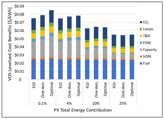
Figure 2.
Value of Solar (VOS) for south-facing 41° tilt (41S), horizontal one-axis tracking (One-Axis), and optimal fixed orientation (Optimal) systems. VOS is broken down into fuel, variable operation and maintenance (VOM), capacity credit, fixed operations and maintenance (FOM), transmission and distribution (T&D), transmission losses, and environmental carbon credit (CO2). The optimal fixed orientation produces highest energy-normalized VOS in most cases.
The energy-normalized VOS is highest for the optimal fixed orientation, which achieves the highest capacity credit. The slightly higher fuel and VOM benefits of the optimal fixed orientation indicate that more of the peak energy (i.e., displaced CT energy) is being met by solar compared to the other orientations. What is not captured with the energy-normalized VOS is the total annual energy produced by the optimal fixed orientation is the lowest, while the one-axis orientation produces the highest annual energy. This is addressed by considering the capacity-normalized VOS based on annual benefits, as well as the levelized annual costs (LAC) for PV installation [38].
Combined VOS and LAC are presented in Figure 3 as capacity-normalized annual benefits/costs ($/kW). VOS is plotted as positive and LAC as negative, such that their sum is the net value. The one-axis system has the highest capacity-normalized VOS, owing to its highest annual energy production. However, the one-axis system also has the highest LAC due to the added complexity of tracking. When VOS and LAC are combined to yield the net value, the optimal fixed orientation remains the highest. The net value at marginal PV contribution (0.1%) is large and negative because PV costs per capacity are higher in small systems. The net value is also negative at high PV energy contribution (25%) due to a decreasing capacity credit of the system VOS. The 4% PV case has the highest normalized net benefit since VOS remains high while the PV cost per capacity is substantially less than the marginal (0.1%) case.
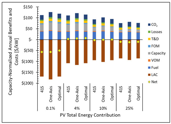
Figure 3.
Capacity normalized annual ($/kW) combined Value of Solar (VOS), Levelized Annual Cost (LAC), and net value (VOS—LAC) for south-facing 41° tilt (41S), horizontal one-axis tracking (One-Axis), and optimal fixed orientation (Optimal) systems. VOS is broken down into fuel, variable operation and maintenance (VOM), capacity credit, fixed operations and maintenance (FOM), transmission and distribution (T&D), transmission losses, and environmental carbon credit (CO2).
Production data model VOS results are compared to TMY solar prediction from PVWatts [36]. TMY VOS was calculated for a fixed 41° tilt south-facing system, one-axis tracker, and an optimized fixed orientation. The results are presented in Figure 4 as the difference between the production data model and TMY, where a positive result means the production data model VOS is higher. Except for the marginal (0.1%) one-axis case, the production data VOS consistently has a higher capacity credit than TMY, representing the largest categorical difference. The 8% capacity credit difference and nearly 12% total difference at low PV energy contribution (4%) stand out as particularly significant and supporting evidence of a strong correlation between maximum PV system generation and peak municipal energy demand. In the 4 and 10% one-axis cases, the difference is split by component with fuel, VOM, and carbon credit as negative, while the capacity credit, FOM, and T&D differences are positive. This results from higher total annual energy for the one-axis TMY prediction than the production data model (see Table A1). The total VOS difference in these cases remains positive due to higher production data capacity credit. The total VOS difference is negative for the 25% PV contribution since the production data model results in more over-production than TMY, which makes energy-based cost differences net negative for all orientations.
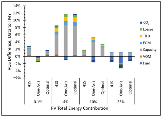
Figure 4.
Difference in Value of Solar (VOS) for the production data model versus Typical Meteorological Year (TMY) solar prediction. Differences in category (fuel, VOM, capacity, etc.) are plotted as negative or positive, with positive indicating that production model VOS is higher than TMY prediction.
The underlying cause of the VOS difference between the production data model and TMY prediction is compared in more detail in Figure 5 for the optimal fixed orientation systems. The comparison is based off the Residual Load Duration Curve (RLDC) for each scenario such that residual conventional generation can be broken down into base, intermediate, and peak generation. The difference between the RLDC and original LDC peak demand is the capacity credit. The capacity credit decreases quite dramatically with increasing PV energy contribution from over 65% in the marginal (0.1%) case to less than 15% in the high PV energy contribution case. The relative reduction in the peak generation capacity is highest for 4% PV energy contribution, and the capacity credit transitions to more displaced base generation at 25% PV energy contribution. Comparing the production data model and TMY prediction, the largest difference is in the 4% PV energy case, where the production data model capacity credit remains over 60% while the TMY prediction is closer to 40%. This difference explains much of the 12% VOS difference observed in Figure 4. Another key observable difference between the production data model and TMY prediction is the production data model has a consistently lower RLDC peak capacity, which is again evidence of the correlation between maximum PV system generation and high municipal energy demand.
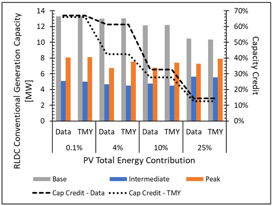
Figure 5.
Residual Load Duration Curve (RLDC) conventional generation capacities for the optimal Value of Solar (VOS) fixed orientation system. Solar capacity credit is above 60% for PV energy contribution less than 4% but decreases to below 15% for 25% PV energy contribution. Base generation is most significantly reduced at 25% PV energy contribution.
3.2. Orientation Optimization
Alternate TOU and ROU rates were set following the methods outlined in the 2.4 Alternate Rate Structures section. The resulting equivalent revenue base rates are shown in Table 4. Multipliers for intermediate and peak rates were set at 1.4 and 2.1, respectively, based on the relative levelized costs for intermediate and peak conventional generation energy as defined by the municipal LDC (see Figure A2). These multipliers are consistent with published TOU rate structures in California and Ontario, Canada [39,40]. Based on the LDC, the SCMU ROU base rate is applied for a demand less than 13,322 kW, the peak rate is triggered above 18,417 kW, and the intermediate rate is charged in between. The average hourly consumption plots for SCMU and the base/intermediate/peak conventional generation costs that inform these rate designs are included in Figure A2 and Figure A3.
Table 4.
Time-of-Use (TOU) and Rate-of-Use (ROU) energy costs for base, intermediate, and peak energy. Energy costs were calculated to generate revenue equivalent to the existing demand/energy rate (D/E) structure over the five years of analysis. Resulting rates are similar for TOU and ROU structures at 0.06–0.07 $/kWh for base energy and 0.013–0.014 $/kWh for peak energy.
With the optimal fixed orientation achieving the highest net value of the VOS less LAC, the optimal orientation (azimuth, tilt) and annual PV system savings for the different electric rate structures are compared to the benchmark VOS results. Optimal azimuth and tilt angles are shown in Figure 6. Demand-dependent VOS and D/E systems favor a more southwest facing system at lower PV energy contributions, up to 225° azimuth. Only at 25% PV energy contribution does the optimal azimuth consistently stay within 10° of south as found in other VOS studies [23]. The Time-of-Use (TOU) optimal orientation is nearly constant, owing to the time-dependent nature of the rate structure and known temporal position of the sun. The optimal evening (TOUe) azimuth is 10° further west than midday (TOUm). The production data modeling and TMY results are overall similar and follow the same trends per rate structure. There is not significant tilt variation amongst the design optimizations, as all tilts of all systems are between 30 and 40° from horizontal and somewhat concentrated near the 37° found to maximize total hourly irradiation [22]. However, one interesting observation is that the optimal TMY tilt is consistently 3–5° higher than the corresponding optimal tilt of the production data model.
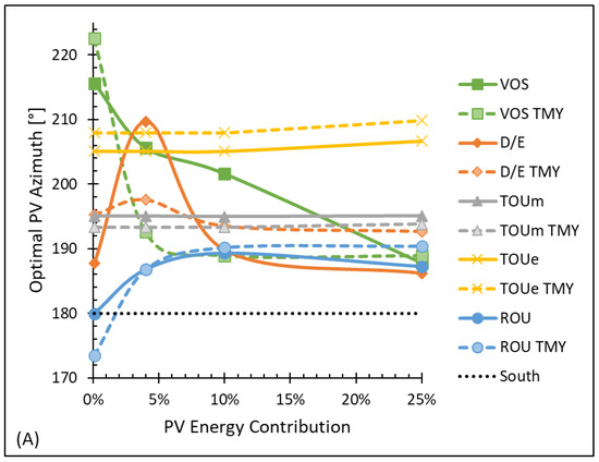
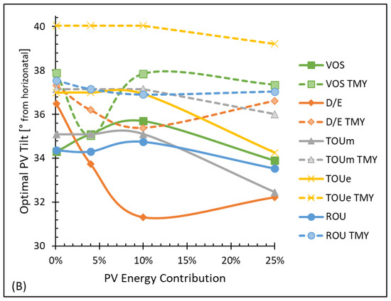
Figure 6.
Comparison of optimal azimuth (plot (A)) and tilt (plot (B)) angles for production data model and Typical Meteorological Year (TMY) for Value of Solar (VOS), as well as demand/energy (D/E), Time-of-Use midday (TOUm), TOU evening (TOUe), and Rate-of-Use (ROU) energy rate structures. With small differences in specific azimuth angles, in general, the trends remain the same: VOS and D/E favor a south-southwest-facing system with an optimal azimuth that decreases with increasing PV energy contribution, while TOU rate structures maintain a constant optimal azimuth with the TOUe favoring a more southwest direction than TOUm. Tilt is less of an orientation factor than azimuth as all the optimal configurations lie between 30 and 40° tilt. However, there is a consistent trend where the optimal production data tilt is 3–5° less than the corresponding TMY optimization.
The capacity-normalized ($/kW) annual cost savings of the optimal fixed orientation PV system are presented in Figure 7 for different rate structures. The D/E and ROU savings trend down with increasing PV energy, consistent with observations in the VOS. The TOU savings stay flat with increasing PV contributions because they are sensitive to the time of energy generation rather than the capacity/rate of energy generation. The ROU savings are consistently the highest, while D/E overall agrees best with the VOS benchmark. The extra D/E marginal (0.1%) PV savings can provide some economic incentive to overcome the negative net value for small-capacity installations noted in Figure 3.
Figure 7.
Optimal fixed orientation annual cost savings capacity normalized ($/kW) for Demand/Energy (D/E), Time-of-Use midday (TOUm) and evening (TOUe), and Rate-of-Use (ROU) energy structures compared to the Value of Solar (VOS) benchmark. D/E and ROU savings trend down with increasing PV energy similar to VOS, while TOU savings remains flat. ROU savings are consistently the highest. Error bars represent 90% confidence intervals from Monte Carlo simulations.
The plotted uncertainty of the annual cost savings is based upon the uncertainty of the production data and production model error. Production model regression curves of the verification and validation data are included in Figure A4 and found to be less than 2.3% RMSE of rated capacity and less than 1.2% error in total annual energy generated (see Table A1). The 90% confidence interval error bars on the plots are based on the converged Monte Carlo simulations shown in Figure A5.
The production data modeling of annual costs savings are compared to the TMY prediction and presented as a difference in Figure 8 where positive means the production data model savings are greater. The same 12% difference in VOS identified in Figure 4 is also shown Figure 8. For this same 4% PV energy contribution case, there is also a 6% advantage of the production data model of D/E annual savings. Another large 11% advantage is observed for D/E in the marginal PV energy contribution case. TOU and ROU have small differences in savings in nearly all cases, while D/E maintains a statistically significant advantage through 10% PV energy contribution. For the 25% PV energy contribution case, all rate structures have savings less than the TMY, which is attributed to increased overproduction.
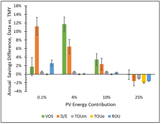
Figure 8.
Comparison of annual cost savings for the production data model and Typical Meteorological Year (TMY) solar prediction. The 90% confidence interval uncertainty confirms a statistically significant savings difference for Value of Solar (VOS) and demand/energy (D/E), which are most dependent on PV production during specific instances of peak demand. Time-of-Use midday and evening (TOUm, TOUe) show little difference since they are more dependent on total annual energy production which was intentionally equalized. The high 25% PV energy contribution shows a negative difference due to increased PV overproduction as the TMY production tends to be more levelized day-to-day.
3.3. Investment Analysis
The PV investment analysis results are summarized in Table 5. The simple payback is shortest for the 4% PV energy case at 13 years and is the longest for the 25% PV energy case at 22 years. For the zero NPV analysis, a positive RROE was found for all cases, except the 25% PV energy contribution, which is slightly negative. The 4% PV case yields a 13% RROE, corresponding to a 7.5% nominal WACC, indicating that installing PV is a sound financial investment. This analysis assumes an overnight install at the optimal PV orientation for each level of PV contribution. It is possible that higher rate-of-returns could be obtained for incremental capacity installations at corresponding optimal PV orientations.
Table 5.
Investment analysis and rate-of-return for PV investment. A simple payback was calculated based on total PV installation costs and annual cost savings. A zero net present value (NPV) analysis was run to calculate the Rate-of-Return on Equity (RROE) and corresponding Weighted Average Cost of Capital (WACC) over the 25-year period of performance. The 4% PV energy contribution has the shortest simple payback and highest RROE and WACC. The RROE of the 25% PV energy contribution is negative to achieve a zero NPV.
RROE is highest for the 4% PV energy contribution, which is notable since SCMU’s current energy portfolio includes 4% wind energy [27]. Thus, these results indicate that investment in PV makes sense from a financial standpoint in addition to the system energy and capacity value provided by mixed RES generation.
4. Conclusions
Value of Solar (VOS) effectively measures the net system benefit provided by PV as total grid energy contribution is increased. VOS is calculated from real PV production data and found to be up to 12% higher than TMY predictions due to the higher capacity credit indicative of a significant correlation between the maximum PV generation and the peak utility demand. VOS is calculated for a northwest Iowa municipal utility representative of the upper Midwest USA geographically and found to exceed the levelized annual costs of installation for low (4%) and medium (10%) PV energy contribution. VOS results can be used by decision makers to inform policies regarding PV installation incentives and local electric rates for both consumption and generation.
Leveraging VOS as a benchmarking optimization tool, a demand/energy rate structure is shown to best match VOS in terms of its economic value and optimal orientation as PV energy contribution is increased. A 25-year net present value (NPV) economic analysis indicates that PV energy is a sound investment up to and beyond a 4% energy contribution that equals the current wind contribution of the utility’s energy portfolio. Given the high-capacity credit of lower PV energy contribution installations, there is opportunity to meet short-term peak demand growth with cleaner PV energy while delaying and/or eliminating the need to build new fossil-based generation plants. As energy storage and other renewable energy enabling technology continues to grow in capability and decrease in cost, adding more PV capacity to the upper Midwest generation portfolio makes good social, environmental, and economic sense.
Author Contributions
Conceptualization, B.A.S. and J.C.Q.; methodology, B.A.S. and J.C.Q.; software, B.A.S.; validation, B.A.S.; formal analysis, B.A.S.; investigation, B.A.S.; resources, J.C.Q.; writing—original draft preparation, B.A.S.; writing—review and editing, J.C.Q.; visualization, B.A.S. and J.C.Q.; supervision, J.C.Q. All authors have read and agreed to the published version of the manuscript.
Funding
This research received no external funding.
Data Availability Statement
All data are available directly from the authors.
Acknowledgments
The authors wish to acknowledge Sioux Center Municipal Utilities for providing the municipal electric demand data, Dordt University for the PV generation data used to conduct this study, and the Quinn Research Group.
Conflicts of Interest
The authors declare no conflict of interest.
Abbreviations
| ATB | Annual Technology Baseline |
| CAPEX | Capital Expenditures |
| CC | Combined Cycle |
| CT | Combustion Turbine |
| CF | Capacity Factor |
| DF | Debt Fraction |
| FCR | Fixed Charge Rate |
| FOM | Fixed Operation and Maintenance |
| IR | Interest Rate |
| LAC | Levelized Annual Cost |
| LCOE | Levelized Cost of Energy |
| LDC | Load Duration Curve |
| MACRS | Modified Accelerated Cost Recovery System |
| NPV | Net Present Value |
| NREL | National Renewable Energy Lab |
| PV | Photovoltaic |
| RES | Renewable Energy Systems |
| RLDC | Residual Load Duration Curve |
| RMSE | Root Mean Square Error |
| ROU | Rate-of-Use |
| RROE | Rate of Return on Equity |
| SCMU | Sioux Center Municipal Utilities |
| SSW | South-Southwest |
| T&D | Transmission and Distribution |
| TOUm | Time-of-Use midday |
| TOUe | Time-of-Use evening |
| TMY | Typical Meteorological Year |
| TR | Tax Rate |
| U.S. EIA | United States Energy Information Administration |
| VOM | Variable Operation and Maintenance |
| VOR | Value of Resource |
| VOS | Value of Solar |
| WACC | Weighted Average Cost of Capital |
| WWSIS | Western Wind and Solar Integration Study |
Appendix A
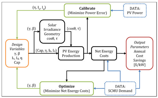
Figure A1.
PV optimization system model diagram showing input data of electric load/demand and PV Power. Two iterative processes are leveraged. First, the energy production model is calibrated to best fit the PV production data. Then, the PV system orientation is optimized to maximize energy cost savings.
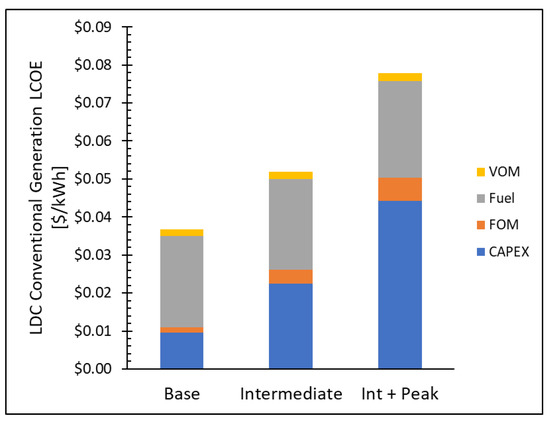
Figure A2.
Comparative conventional generation Levelized Cost of Energy (LCOE) for base, intermediate, and peak loads based on the Load Duration Curve (LDC). Costs are broken down into categories of capital expenditures (CAPEX), fixed operations and maintenance (FOM), fuel, and variable operations and maintenance (VOM). CAPEX and FOM fixed costs represent an increasing portion of the total cost for intermediate and peak generation. The calculated cost ratios of 1.4 for intermediate to base and 2.1 for intermediate/peak to base agree well with published time-of-use rate structures [39,40].
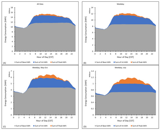
Figure A3.
Hourly energy consumption broken down into base, intermediate, and peak types from the Load Duration Curve (LDC). Graph (A) is the entirety of the five years of load data, while graph (B) shows the increased commercial/industrial load on weekdays. Graphs (C,D) demonstrate the increased peak demand from late spring to early fall, peaking specifically in July.
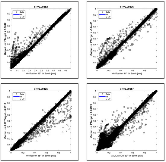
Figure A4.
Verification and validation regression plots for 16, 29, 41, and 65° tilt, south-facing production data. The production model is calibrated and verified with 16, 41, and 65° tilt data and then validated with the 29° tilt production data.
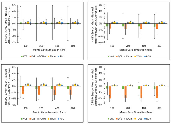
Figure A5.
Convergence of the Monte-Carlo simulation as runs are increased from 100 to 800 for each of the 0.1, 4, 10, and 25% PV energy contribution scenarios. Results are plotted as percent difference of Monte Carlo simulation mean compared to nominal annual cost savings. Value of Solar (VOS) and Demand/Energy (D/E) rate have a negative bias in simulation savings beyond the 0.1% PV energy marginal scenario, while the Time-of-Use (TOU) and Rate-of-Use (ROU) have slight positive bias. The 90% confidence interval error bars are greater for VOS and D/E rate due to their cost sensitivity to instances of peak demand. The span of VOS and D/E confidence interval also decreases with increased PV energy contribution as a higher portion of total cost savings is attributed to energy than demand.
Table A1.
Annual production (kWh/kW) for installed PV compared to PVWatts Typical Meteorological Year (TMY) prediction. PVWatts DC losses were lowered to 11% from the default 14% to best match the annual production. Also included for comparison to the raw data is the production data model of annual production.
| Configuration | Data Annual Energy [kWh/kW] | TMY Annual Energy [kWh/kW] | TMY to Data Difference | Production Data Model Annual [kWh/kW] | Model to Data Difference |
|---|---|---|---|---|---|
| South, 16° Tilt | 1383 | 1390 | +0.5% | 1400 | +1.2% |
| South, 29° Tilt | 1459 | 1464 | +0.3% | 1465 | +0.4% |
| South, 41° Tilt | 1476 | 1479 | +0.2% | 1475 | −0.1% |
| South, 65° Tilt | 1366 | 1359 | −0.5% | 1355 | −0.8% |
| One-Axis Tracking | - | 1616 | - | 1571 | - |
References
- U.S. EIA. Electricity: Detailed State Data 2021. Available online: https://www.eia.gov/electricity/data/state/ (accessed on 28 June 2021).
- U.S. EIA. Annual Energy Outlook 2020 with Projections to 2050; U.S. Energy Information Administration: Washington, DC, USA, 2020.
- Bloom, A.; Townsend, A.; Palchak, D.; Novacheck, J.; King, J.; Barrows, C.; Ibanez, E.; O’Connell, M.; Jordan, G.; Roberts, B.; et al. Eastern Renewable Generation Integration Study; TP-6A20-64; National Renewable Energy Laboratory: Golden, CO, USA, 2016.
- Miller, N.W.; Shao, M.; Pajic, S.; D’Aquila, R. Western Wind and Solar Integration Study Phase 3: Frequency Response and Transient Stability; National Renewable Energy Laboratory: Golden, CO, USA, 2014; pp. 1–213.
- Lew, D.; Piwko, D.; Miller, N.; Jordan, G.; Clark, K.; Freeman, L. How Do High Levels of Wind and Solar Impact the Grid? The Western Wind and Solar Integration Study; TP-5500-50057; National Renewable Energy Laboratory: Golden, CO, USA, 2010; pp. 1–11.
- Hirth, L.; Ueckerdt, F.; Edenhofer, O. Integration costs revisited—An economic framework for wind and solar variability. Renew. Energy 2015, 74, 925–939. [Google Scholar] [CrossRef]
- Heptonstall, P.J.; Gross, R.J.K. A systematic review of the costs and impacts of integrating variable renewables into power grids. Nat. Energy 2021, 6, 72–83. [Google Scholar] [CrossRef]
- Lew, D.; Miller, N.; Clark, K.; Jordan, G. Impact of High Solar Penetration in the Western Interconnection; National Renewable Energy Laboratory: Golden, CO, USA, 2010; pp. 1–9.
- Taylor, M.; McLaren, J.; Cory, K.; Davidovich, T.; Sterling, J.; Makhyoun, M. Value of Solar: Program Design and Implementation Considerations; National Renewable Energy Laboratory: Golden, CO, USA, 2015.
- National Association of Regulatory Utility Commissioners. Distributed Energy Resources Rate Design and Compensation; National Association of Regulatory Utility Commissioners: Washington, DC, USA, 2016. [Google Scholar]
- U.S. EIA. Levelized Cost and Levelized Avoided Cost of New Generation Resources in the Annual Energy Outlook 2020; U.S. Energy Information Administration: Washington, DC, USA, 2020.
- U.S. EIA. Assumptions to the Annual Energy Outlook 2020: Electricity Market Module; U.S. Energy Information Administration: Washington, DC, USA, 2020.
- Denholm, P.; Margolis, R.; Palmintier, B.; Barrows, C.; Ibanez, E.; Bird, L. Methods for Analyzing the Benefits and Costs of Distributed Photovoltaic Generation to the U.S. Electric Utility System; National Renewable Energy Laboratory: Golden, CO, USA, 2014.
- O’Shaughnessy, E.; Ardani, K. Distributed rate design: A review of early approaches and practical considerations for value of solar tariffs. Electr. J. 2020, 33, 106713. [Google Scholar] [CrossRef]
- Zummo, P. Rate Design for Distributed Generation Net Metering Alternatives With Public Power Case Studies; American Public Power Association: Arlington, VA, USA, 2015. [Google Scholar]
- Zummo, P.; Cartes, J.; Cater, J. Rate Design Options for Distributed Energy Resources; American Public Power Association: Arlington, VA, USA, 2016. [Google Scholar]
- Hansen, L.; Lacy, V.; Glick, D. A Review of Solar PV Benefit and Cost Studies; Rocky Mountain Institute (RMI): Basalt, CO. USA, 2013; Volume 59. [Google Scholar]
- Brown, P.R.; O’Sullivan, F.M. Spatial and temporal variation in the value of solar power across United States electricity markets. Renew. Sustain. Energy Rev. 2020, 121, 109594. [Google Scholar] [CrossRef]
- Schulte, R.H.; Fletcher, F.C. Why individual electric utilities cannot achieve 100 % clean energy. Electr. J. 2021, 34, 106909. [Google Scholar] [CrossRef]
- Cole, W.; Frazier, A.W. Impacts of increasing penetration of renewable energy on the operation of the power sector. Electr. J. 2018, 31, 24–31. [Google Scholar] [CrossRef]
- MATLAB. R2019b Update 5 (9.7.0.1319299); The Mathworks Inc.: Natick, MA, USA, 2020. [Google Scholar]
- Lave, M.; Kleissl, J. Optimum fixed orientations and benefits of tracking for capturing solar radiation in the continental United States. Renew. Energy 2011, 36, 1145–1152. [Google Scholar] [CrossRef] [Green Version]
- Rhodes, J.D.; Upshaw, C.R.; Cole, W.J.; Holcomb, C.L.; Webber, M.E. A multi-objective assessment of the effect of solar PV array orientation and tilt on energy production and system economics. Sol. Energy 2014, 108, 28–40. [Google Scholar] [CrossRef] [Green Version]
- Milligan, M.; Ela, E.G.; Hodge, B.-M.S.; Kirby, B.; Lew, D.; Clark, C.; Decesaro, J. Integration of Variable Generation, Cost-Causation, and Integration Costs. Electr. J. 2011, 24, 51–63. [Google Scholar] [CrossRef]
- GE Energy. Western Wind and Solar Integration Study; National Renewable Energy Laboratory: Golden, CO, USA, 2010.
- Lew, D.; Brinkman, G.; Ibanez, E.; Hodge, B.; King, J. The western wind and solar integration study phase 2. Contract 2013, 303, 275–3000. [Google Scholar]
- Missouri River Energy Services. MRES Energy Resources Generation 2020. Available online: https://www.mrenergy.com/energy-resources/generation (accessed on 10 March 2022).
- Ueckerdt, F.; Hirth, L.; Luderer, G.; Edenhofer, O. System LCOE: What are the costs of variable renewables? Energy 2013, 63, 61–75. [Google Scholar] [CrossRef]
- EBP US. Failure to Act: Electric Infrastructure Investment Gaps in a Rapidly Changing Environment, 2020; EBP US: Boston, MA, USA, 2020. [Google Scholar] [CrossRef] [Green Version]
- U.S. EIA. Natural Gas Explained: Natural Gas and the Environment 2020. Available online: https://www.eia.gov/energyexplained/natural-gas/natural-gas-and-the-environment.php (accessed on 15 October 2020).
- Lew, D.; Brinkman, G.; Kumar, N.; Besuner, P.; Agan, D.; Lefton, S. Impacts of Wind and Solar on Fossil-Fueled Generators. In Proceedings of the IEEE Power and Energy Society General Meeting, San Diego, CA, USA, 22–26 July 2012; pp. 1–8. [Google Scholar]
- U.S. Government. Technical Support Document: Technical Update of the Social Cost of Carbon for Regulatory Impact Analysis under Executive Order No. 12866; Office of Management and Budget: Washington, DC, USA, 2015; pp. 65–88.
- Black & Veatch. Power Plant Engineering; Chapman & Hall: New York, NY, USA, 1996. [Google Scholar]
- Perez, R.; Ineichen, P.; Seals, R.; Michalsky, J.; Stewart, R. Modeling daylight availability and irradiance components from direct and global irradiance. Sol. Energy 1990, 44, 271–289. [Google Scholar] [CrossRef] [Green Version]
- Dobos, A.P. PVWatts Version 5 Manual (NREL/TP-6A20-62641); U.S. Energy Information Administration: Washington, DC, USA, 2014; Volume 20. [CrossRef] [Green Version]
- NREL. NREL’s PVWatts® Calculator 2019. Available online: http://pvwatts.nrel.gov/ (accessed on 8 May 2020).
- NREL. Equations and Variables in ATB. Annual Technology Baseline 2021. Available online: https://atb.nrel.gov/electricity/2021/equations_&_variables (accessed on 10 March 2022).
- Feldman, D.; Ramasamy, V.; Fu, R.; Ramdas, A.; Desai, J.; Margolis, R. U.S. Solar Photovoltaic System and Energy Storage Cost Benchmark: Q1 2020; National Renewable Energy Laboratory: Golden, CO, USA, 2021; pp. 1–120.
- Southern California Edison. Time-of-Use (TOU) Rate Plans 2021. Available online: https://www.sce.com/residential/rates/Time-Of-Use-Residential-Rate-Plans (accessed on 5 June 2021).
- Hydro One. Electricity Pricing and Costs 2021. Available online: https://www.hydroone.com/rates-and-billing/rates-and-charges/electricity-pricing-and-costs (accessed on 5 June 2021).
Publisher’s Note: MDPI stays neutral with regard to jurisdictional claims in published maps and institutional affiliations. |
© 2022 by the authors. Licensee MDPI, Basel, Switzerland. This article is an open access article distributed under the terms and conditions of the Creative Commons Attribution (CC BY) license (https://creativecommons.org/licenses/by/4.0/).