Modeling, Validation, and Analysis of a Concentrating Solar Collector Field Integrated with a District Heating Network

Abstract

In recent years, concentrating solar collectors have been integrated with several district heating systems with the aim of taking advantage of their low heat losses. The present study investigates the Brønderslev combined heat and power plant, which consists of a 16.6 MW parabolic trough collector field, two biomass boilers, and an organic Rankine cycle system. The study focuses on the solar collector field performance and integration with the district heating network. An in situ characterization of the parabolic solar collector field using the quasi-dynamic test method found that the field had a peak efficiency of 72.7%. Furthermore, a control strategy for supplying a constant outlet temperature to the district heating network was presented and implemented in a TRNSYS simulation model of the solar collector field. The developed simulation model was validated by comparison to measurement data. Subsequently, the simulation model was used to conduct a sensitivity analysis of the influence of the collector row spacing and tracking axis orientation. The results showed that the current suboptimal tracking axis rotation, made necessary by the geography of the location, only reduced the annual power output by 1% compared to the optimal configuration. Additionally, there were only minor improvements in the annual heat output when the row spacing was increased past 15 m (ground cover ratio of 0.38).

1. Introduction

The first solar district heating plants were developed in the 1970s with demonstration plants in Europe and the USA [1]. Since then, solar district heating plants have grown increasingly larger and have experienced significant market growth in Denmark, Germany, Austria, and China [2].

As of 2020, there were 262 large-scale solar district heating systems globally, corresponding to an installed capacity of 1.4 GW [3]. Currently, Denmark leads the market in both number of systems and total installed capacity, with 124 systems in operation. The locations of the active solar heating plants in Denmark are shown with yellow dots in Figure 1 (see http://solarheatdata.eu (accessed on 6 March 2022) for detailed information). All of the plants in Figure 1 are based on flat-plate solar collectors, except for the three highlighted plants. Instead, these three plants utilize concentrating solar collectors (Brønderslev and Lendemarke) or a combination of concentrating and flat-plate collectors (Tårs).

Using concentrating solar collectors for district heating was first investigated in the Nordic region by Karlsson and Hultmark in 1986 [4]. The study concluded that flat-plate collectors were more favorable than concentrating collectors in the district heating temperature range. The main reasons cited were the lower cost of flat-plate collectors and the low amount of direct irradiation in the Nordic region.

Flat-plate collectors are, indeed, less expensive than concentrating collectors, which has led to their widespread usage, further driving down their cost. However, concentrating collectors have certain benefits, especially relating to their low absorber area and, thus, very low heat losses, which make them suitable for producing high-temperature heat [5]. For example, parabolic trough collectors can generate heat up to 400 °C [6]. In contrast, flat-plate collectors have larger absorber areas and, thus, experience much larger heat losses, which cause their efficiency to drop significantly at higher temperatures. For this reason, flat-plate collectors are generally not used for producing heat above 100 °C [2].

Due to their ability to function efficiently at high temperatures, concentrating solar collectors have historically been used for electricity generation, often referred to as concentrated solar power (CSP) [7]. However, in recent years, several commercial actors have investigated how the benefits of concentrating solar collectors can be leveraged in the district heating sector. For instance, multiple companies have attempted to tackle the main challenge of concentrating collectors (i.e., their high cost) by developing innovative manufacturing methods.

The first district heating plant to use concentrating solar collectors was a pilot plant in Thisted, Denmark [8]. The plant operated from 2013 to 2015 and successfully demonstrated that parabolic trough collectors (PTC) can easily be integrated with district heating systems. Based on the experiences from Thisted, a hybrid plant combining parabolic trough collectors and flat-plate collectors was commissioned in 2015 in Tårs, Denmark [5,9]. By utilizing both technologies, each one can be operated in the temperature range where it performs the best. Therefore, in the Tårs plant, the heat transfer fluid (water) is first heated by the flat-plate collector loop, which has a high efficiency in the low-temperature range. In the second stage, the water preheated by the flat-plate collectors is heated to the desired outlet temperature by the parabolic trough collectors, which have a stable efficiency at higher temperatures. Furthermore, in 2016, the Brønderslev hybrid power plant was inaugurated, featuring a field of parabolic trough collectors [10]. The Brønderslev solar collector field can supply heat directly to the district heating grid or to an organic Rankine cycle (ORC) system. The most recent concentrating solar plant in Denmark was built in Lendemarke in 2018 and was based on two-axis tracking Fresnel-lens collectors [11].

Following the demonstration projects in Denmark, several international district heating projects have been realized with concentrating solar collectors – notably in China [12], Sweden [13], and France [14]. All of the identified projects utilize parabolic trough collectors that supply heat directly to a local district heating network. Nevertheless, the literature contains very few studies of concentrating solar collectors integrated with district heating systems.

The present study aimed to elucidate the performance of a concentrating solar collector field integrated with a district heating system. Specifically, the Brønderslev solar field was characterized using the quasi-dynamic test (QDT) method, obtaining the heat loss coefficient, thermal capacity, and peak efficiency. Furthermore, a control strategy for supplying a constant temperature to the district heating network was derived. The control strategy was implemented in a simulation model and validated by comparison with measurement data. The simulation model was subsequently used to identify the impact of changing the field layout, namely the impact of row spacing and tracking axis orientation on the annual yield. Knowledge of how these two parameters impact heat generation is crucial for engineering designs, as the choice of parameters is an economic trade-off.

An overview of the Brønderslev hybrid plant is provided in Section 2, followed by a description of the methods in Section 3. The results of the study are presented in Section 4, and the conclusions are given in Section 5.

2. Brønderslev Hybrid Plant

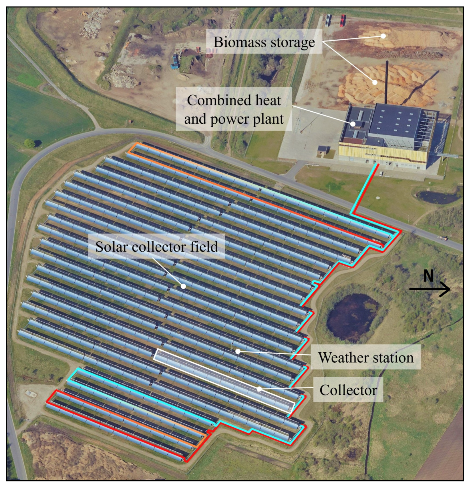
The Brønderslev hybrid plant is a solar-biomass combined heat and power plant (CHP) (see Figure 2). The plant was inaugurated in 2018 and supplies district heating and electricity to the town of Brønderslev in Denmark (latitude: 57.255° N, longitude: 9.955° E). The plant consists of a 16.6 MW_heat concentrating solar collector field, two 10 MW_heat biomass boilers, and a 3.9 MW_el organic Rankine cycle (ORC) turbine. The solar field and biomass boilers utilize the same heat transfer fluid, namely Therminol 66. This allows for the two sources to be directly coupled, i.e., they can both supply heat to the ORC system independently or together. The waste heat, which includes the condenser heat from the ORC and heat recovered from the flue gas, is utilized for district heating.

The district heating network consists of 160 km of pipes and supplies heat to 4800 customers. The average annual heat demand of the town is 122 GWh, with an average supply and return temperature of 74 °C and 35 °C, respectively. The hybrid plant is designed to supply 90% of the town’s district heating needs. The remaining heat is generated from a mix of conventional gas boilers, gas motors, an electric boiler, and industrial waste heat.

2.1. Solar Field

The solar collector field consists of 40 parabolic trough collectors (PTC) and has a peak thermal output of 16.6 MW_heat. The solar field, which covers an area of 9 hectares, was constructed adjacent to the biomass power plant to minimize piping and heat losses. The total mirror (aperture) area is 26,930 m${}^2$, and the row spacing is 15 m. Construction of the solar collector field started in 2016, and the plant began operation in January 2017.

Each collector has a width of 5.77 m and is 120 m long. The PTCs were manufactured by the Danish company Aalborg CSP and are of the type AAL-TroughTM 4.0. Aalborg CSP also delivered the solar field control system and piping. The collectors are single-axis tracking, with a tracking axis 29.9° east of north, and while many studies have shown that a north–south tracking axis maximizes energy output [15], this was not feasible due to the geometrical constraints of the available plot of land (restricted by the road and lake shown in Figure 2).

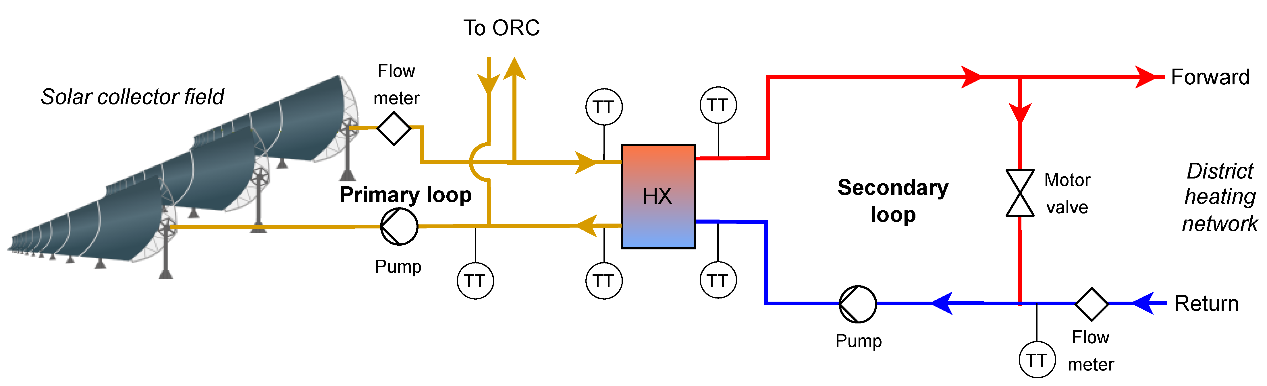
Depending on the incident irradiance and desired output, the solar collector field can be operated in district heating or ORC mode. In the district heating mode, the solar collector field supplies heat directly to the district heating network via a heat exchanger (see Figure 3). In this mode, it is desirable to have an as low as possible outlet temperature to minimize the heat losses in the solar collector field. In the district heating mode, the outlet and inlet temperatures of the solar collector field are around 190 °C and 130 °C, respectively. The ORC, however, requires high-temperature heat; hence, in the ORC mode, the setpoint of the outlet temperature from the solar field is 312 °C, with an inlet temperature around 252 °C. The solar field is in operation whenever the measured direct normal irradiance (DNI) exceeds 150 W/m${}^2$ (42% of daylight periods).

Originally, the plant had received a fixed price subsidy; however, this subsidy was annulled as it was not in compliance with EU regulations. Thus, until a new subsidy was granted in 2020, the solar field was not allowed to supply heat to the ORC. For this reason, there were only a few hours of measurements of joint CSP-ORC operation, which were insufficient to validate a model of the entire system. Therefore, the present study focused on the solar collector field operation in the district heating mode, i.e., direct heat supply to the district heating network.

2.2. Measurement Equipment

A 10 m tower was erected within the solar field to monitor the weather conditions. The tower was equipped with a cup anemometer for measuring the wind speed and a shielded PT100 temperature sensor for measuring the ambient air temperature. The estimated uncertainty of the wind speed was 1.5 m/s, and the uncertainty of the temperature was 0.3 K. The DNI was also measured at the top of the tower using a Class-A pyrheliometer (EKO MS-57) mounted on a solar tracker (EKO STR-21G).

Furthermore, the temperature of the supply and return pipes of the solar collector field and district heating loop were measured using immersed PT100 sensors, with an uncertainty of 0.3 K. The flow in the solar collector field was measured using a Rosemount 485 Annubar flowmeter with an uncertainty ranging from 1 to 3%. The flow on the district heating side was measured with an electromagnetic flowmeter (Siemens SITRANS FM MAG 5000/MAG 3100). The uncertainty of the flow meter on the district heating side was checked annually and found to be below 1.5%. As this analysis only considered the direct supply of heat from the concentrating collector field to the district heating network, the measured thermal power was the same on either side of the heat exchanger. However, since the uncertainty of the thermal power measured on the district heating side was lower, this measurement was utilized in this study.

3. Methods

3.1. Quasi-Dynamic Test (QDT) Method

Solar collectors are generally characterized using the methods described in the international standard ISO 9806 [16]. The standard specifies that only the quasi-dynamic test (QDT) method is suitable for the characterization of concentrating solar collectors. Typically, an individual solar collector is characterized, though it is also of interest to characterize an entire field, as this gives information of the total system. Furthermore, in some cases, such as the Brønderslev solar field, the power generation of the individual collectors is not measured, but only the total power generation of the field is measured. Thus, it is only possible to characterize the entire field performance. Fortunately, with minor modifications, the QDT method can also be applied to solar collector fields [9].

The power output, ${\dot{Q}}_{csp}$, of a solar thermal collector or field can be described using the following equation:

$$\begin{array}{c}\hfill \begin{array}{cc}\hfill \frac{{\dot{Q}}_{csp}}{A}=& {\eta }_{0,b}·K_b({\theta }_L,{\theta }_T)·G_b+K_d·{\eta }_{0,b}·G_d\hfill \\ \hfill & -a_1·(T_{mean}-T_{amb})\hfill \\ \hfill & -a_2·{(T_{mean}-T_{amb})}^2\hfill \\ \hfill & -a_3·u^{\prime }·(T_{mean}-T_{amb})\hfill \\ \hfill & +a_4·(E_L-\sigma ·T_a^4)\hfill \\ \hfill & -a_5·d{T}_{mean}/dt\hfill \\ \hfill & -a_6·u^{\prime }·G_{hem}\hfill \\ \hfill & -a_7·u^{\prime }·(E_L-\sigma ·T_a^4)\hfill \\ \hfill & -a_8·{(T_{mean}-T_{amb})}^4\hfill \end{array}\end{array}$$

(1)

All coefficients are normalized with respect to the collector aperture area (A). A description of the coefficients is provided in [16] and in the nomenclature at the end of the paper.

For one-axis trackers, the incidence angle modifier, $K_b({\theta }_L,{\theta }_T)$, simplifies to $K_b\left({\theta }_L\right)$ as the tracking angle is chosen such that the transversal incidence angle is zero. For parabolic trough collectors, IEC 62862-3-2 [17] recommends using the methodology proposed in [18] for modeling the beam irradiance incidence angle modifier (IAM):

$$K_b\left({\theta }_L\right)=1-\frac{b_1·{\theta }_L+b_2·{\theta }_L^2}{\cos \left({\theta }_L\right)}$$

(2)

The purpose of the QDT method is to identify the unknown collector coefficients in Equation (1): ${\eta }_{0,b}$, $K_d$, $a_1$ through $a_8$, and those of $K_b$. The set of collector coefficient values is unique to a specific collector or system. Once the coefficients have been determined, they can be used to predict the power output under any operating condition. For concentrating collectors, ISO 9806 states that coefficients $a_2$, $a_3$, $a_4$, $a_6$, $a_7$, and $K_d$ may be set to zero [16]. According to the QDT method, the unknown coefficients are determined using multiple linear regression with representative measurement data.

An important consideration when applying the QDT method to large collector fields is the long residence time, i.e., the time it takes the heat transfer fluid (Therminol) to be pumped through the solar collector field. Furthermore, given the setup of the Brønderslev collector field, the residence time varies significantly between the different rows. To smooth out such effects, the data are averaged to 30-min values before determining the coefficients. Furthermore, when using the QDT method, it is vital to select representative and accurate measurement data for the parameter regression. It is particularly critical to ensure that the data include sufficient variability of the input parameters in Equation (1) (particularly the mean fluid temperature and irradiance conditions).

Moreover, to ensure that the pyrheliometer measurements were not strongly influenced by soiling, only the seven following days after each pyrheliometer cleaning were considered. Since the pyrheliometer was infrequently cleaned, this significantly reduced the dataset. In addition, the included days should also have a significant heat production, which was assessed manually. The final dataset consisted of 14 days between May and September 2020. The days included a mix of cloud-free days and days with drifting clouds.

3.2. Model Description

To investigate the solar field performance and its integration with the district heating network, a simulation model was developed in TRNSYS. A schematic of the simulation model is shown in Figure 4. The model consists of several components, also called types, which are documented in [19].

The parabolic trough collector field is modeled using TESS component Type 1289. The component essentially implements Equation (1); thus, the collector coefficients are given as input to the component (although Type 1289 currently does not support $a_7$ and $a_8$). The incidence angle modifier is implemented by interpolating from a 1D user-specified file. The incidence angle file was generated based on Equation (2) with discrete values every 5°. Inter-row shading was modeled using Type 30b, which calculates the unshaded incident irradiance for single-axis tracking collectors.

Furthermore, the heat exchanger is the central part of the model and transfers heat from the hot thermal oil circuit (primary side) to the district heating circuit (secondary side). The heat exchanger is a parallel flow heat exchanger with an active area of 123 m${}^2$ and was modeled using TRNSYS Type 5a. The heat exchanger capacity, k, was modeled using an empirical relationship:

$$k=k_{nom}·{\left(\frac{{\dot{m}}_{csp}}{{\dot{m}}_{csp,nom}}\right)}^{0.45}·{\left(\frac{{\dot{m}}_{dh,hx}}{{\dot{m}}_{dh,hx,nom}}\right)}^{0.45}$$

(3)

where ${\dot{m}}_{csp}$ and ${\dot{m}}_{dh,hx}$ are the mass flow rates on the primary and secondary sides of the heat exchanger, respectively. The nominal values were obtained from the manufacturer’s datasheet: $k_{nom}$ = 1098 W/(m${}^2$ K), ${\dot{m}}_{csp,nom}$ = 98.8 kg/s, and ${\dot{m}}_{dh,hx,nom}$ = 57.3 kg/s. The empirical exponents in Equation (3) were derived from measurements of the Brønderslev plant.

3.2.1. Control Strategy

A minimum flow rate is required through the PTCs during operation to avoid overheating. Similarly, a minimum flow rate is required on the secondary side of the heat exchanger to prevent boiling. Moreover, as shown in the system schematic in Figure 3, there is a bypass loop on the secondary side. The bypass loop is necessary for controlling the temperature of the fluid supplied to the district heating network. Specifically, the bypass loop allows water to be recirculated until the outlet temperature from the heat exchanger matches the district heating setpoint. As the heat transfer in the heat exchanger increases, the flow diverter is gradually adjusted to divert more flow to the district heating network (less recirculation), thus maintaining a constant outlet temperature. At a certain point, all of the flow will be diverted to the district heating network (no recirculation); after this point, the flow rate through the heat exchanger can be increased above the minimum flow to maintain a constant outlet temperature. The necessary flow rate through the heat exchanger, ${\dot{m}}_{dh,hx}$, to achieve the desired outlet temperature can be determined based on the concept of a feed-forward controller:

$${\dot{m}}_{dh,hx}=\max \left(\frac{{\dot{Q}}_{hx,i-1}}{(T_{dh,out,set}-T_{dh,in})·c_{p,dh}},{\dot{m}}_{dh,hx,min}\right)$$

(4)

where $T_{dh,out,set}$ is the desired district heating outlet temperature, $T_{dh,in}$ is the return temperature from the district heating network, ${\dot{Q}}_{hx,i-1}$ is the heat transferred in the heat exchanger at the previous time step, and $c_{p,dh}$ is the specific heat capacity. The minimum flow rate, ${\dot{m}}_{dh,hx,min}$, is set to 42 kg/s to match the actual system enforced constraint. It should also be noted that the secondary side is only active when the primary side is, i.e., ${\dot{m}}_{dh,hx}=0$ if ${\dot{m}}_{csp}=0$.

The fraction of recirculated flow, $f_{rec}$, can be calculated based on the assumption that all of the heat transferred through the heat exchanger has to be delivered to the district heating network (assuming negligible heat capacity of the heat exchanger and bypass loop). The recirculation fraction can be formulated as:

$$f_{rec}=1-\min \left(\frac{{\dot{Q}}_{hx,i-1}}{{\dot{m}}_{dh,hx,min}·(T_{dh,out,set}-T_{dh,in})·c_{p,dh}},1\right)$$

(5)

The mass flow rate of water that is diverted to the district network can then be calculated from the recirculation fraction:

$${\dot{m}}_{dh}={\dot{m}}_{dh,hx}·(1-f_{rec})$$

(6)

Similarly, the flow rate through the solar collector field, $m_{csp}$, can be calculated from Equations (7) and (8):

$${\dot{m}}_{csp,calc}=\frac{{\dot{Q}}_{csp}}{(T_{csp,out,set}-T_{csp,in,i})·c_{p,csp}}$$

(7)

$${\dot{m}}_{csp}=\min \left(\max ({\dot{m}}_{csp,calc},{\dot{m}}_{csp,min}),{\dot{m}}_{csp,max}\right)$$

(8)

where $T_{csp,out,set}$ and $T_{csp,in,i}$ are the outlet setpoint temperature and inlet temperature to the CSP loop, respectively. The upper and lower limits of the mass flow rate in the primary loop are ${\dot{m}}_{csp,max}=$118 kg/s and ${\dot{m}}_{csp,min}$=70 kg/s. The maximum flow rate corresponds to the maximum flow rate the pumps can deliver, whereas the lower limit is imposed to avoid overheating.

3.2.2. Model Validation

To verify that the simulation model performs as expected and with sufficient accuracy, the model was validated. Validation was achieved by simulating a period where the boundary conditions and system behavior were known; thus, the measured parameters, including the direct normal irradiance, were provided as an input to the model, and the predicted and measured power output and temperatures were compared. Additional inputs to the model included the measured wind speed, air temperature, mass flow rate of the solar field, district heating inlet temperature, and the incidence angle. The outlet district heating setpoint temperature was set to 88 °C, and the outlet temperature and flow rates were calculated using the implemented control strategy.

The validation period was selected from 5 May to 31 October 2020, as the pyrheliometer was frequently cleaned during this period, and the period was long enough to include variable weather conditions. The validation simulation was executed with a 1-min time step.

3.2.3. Annual Simulation

An annual simulation using the TRNSYS model was conducted to determine the expected annual performance. A typical meteorological year (TMY) data file for Northern Jutland was used (annual DNI of 1151 kWh/m${}^2$). The TMY file was created by the Danish Meteorological Institute based on ten years of measurement data from the Tårs meteorological station, located 17 km from Brønderslev [20]. The wind speed, ambient temperature, and irradiance were passed to the appropriate components, as shown in Figure 4. The outlet district heating temperature was set to 88 °C, and a constant inlet temperature of 38 °C was used. A temperature of 190 °C was used for the solar field outlet set point.

For the annual simulation, a feed-forward controller based on Equations (7) and (8) was implemented to calculate the flow rate in the CSP loop. The flow rate was maintained within the minimum and maximum limits. The tracker position and incidence angle were calculated by the TMY weather data processor (Type 15-2). The annual simulation was run with a 10-min time step, and the hourly weather data were linearly interpolated.

3.3. Sensitivity Study

The two main defining parameters of the solar collector field layout are the row-to-row distance and the tracking axis azimuth orientation. It is necessary to understand the impact of these defining parameters to determine the optimal plant configuration. Therefore, the present study presents a sensitivity analysis of the annual energy yield as a function of row spacing and azimuth angle. Simulations were carried out for row spacings for every 1 m between 7 and 30 m and axis azimuth angles for every 5° between 0° and 180°. The range of row spacings corresponds to ground cover ratios (GCR) between 0.19 and 0.82, which cover almost all existing systems. All other parameters were maintained the same to match the Brønderslev solar collector field as described in Section 2.1 and Section 3.2.

4. Results

The results of the QDT characterization are presented in Section 4.1, along with a comparison of the findings for similar PTCs. Section 4.2 presents the validation of the simulation model, followed by the results of the annual simulation in Section 4.3 and the sensitivity study in Section 4.4.

4.1. Solar Collector Field Characterization

The collector coefficients identified from the QDT method are listed in

Table 1. Performance coefficients for the Brønderslev solar collector field derived using the QDT method.

Parameter	Value	Std. Dev.	T-Score	Unit
${\eta }_{0,b}$	72.7%	0.6%	113	-
$a_1$	0.271	0.032	8.5	W/(m${}^2$ K)
$a_5$	6741	146	46	J/(m${}^2$ K)
$b_1$	2.6 × 10${}^{-3}$	0.1 × 10${}^{-3}$	25	(°)${}^{-1}$

. The table also includes the standard deviation and t-score for each parameter. According to the QDT method, parameters with a t-score less than three should be omitted, which was the case for $a_2$, $a_8$, and $b_2$.

It is important to note that the coefficients in Table 1 correspond to the entire collector field, including approximately 1200 m of piping that connects the solar collector loops to the power plant. Specifically, this means that the heat loss coefficient ($a_1$) accounts for the heat losses from the PTCs and the pipes, and the heat capacity ($a_5$) includes the additional thermal capacity of the fluid in the pipes and the piping itself.

The impact of the coefficients listed in Table 1, as well as the influence of shading and incidence losses, are illustrated in Figure 5. The figure shows the DNI for a clear-sky day, the magnitude of the various losses, and the useful heat generation. The incidence loss represents the reduction in irradiance caused by the collector surface not being oriented normal to the sun. Due to the tracking axis orientation, the incidence loss is relatively low during the morning; however, in the afternoon, the sun azimuth aligns with the tracking axis resulting in large incidence angles. This gives rise to the bimodal production profile (useful heat). The largest loss is the optical loss, which corresponds to the peak efficiency parameter (${\eta }_{0,b}$) in Table 1 (also sometimes called the optical efficiency). The heat losses from the collector field are also visualized in Figure 5, which are relatively small compared to the other losses.

The coefficients determined for the Brønderslev solar collector field are compared to values from similar PTCs in

Table 2. Comparison of performance coefficients for different parabolic trough collectors.

Parameter	Brønderslev (Full Scale)	Brønderslev (Pilot Plant) [21]	Tårs [9]	EUROtrough [22]	Unit
${\eta }_{0,b}$	72.7%	75.0%	73.6%	72.2%	-
$a_1$	0.271	0.06	0.04	0.192	W/(m${}^2$ K)
$a_5$	6741	-	2962	1749	J/(m${}^2$ K)
$a_8$	-	-	-	8.33 × 10${}^{-8}$	W/(m${}^2$ K${}^4$)

. For example, the collector coefficients determined for the Brønderslev pilot plant are reported. In the pilot study [21], two collectors were constructed on the site of the full-scale plant as a proof of concept and to validate the performance. The slightly higher value found for the peak efficiency for the pilot plant is likely because the mirrors and receivers were clean during the pilot study. In comparison, the present study used data for 2020, when the collectors had been exposed to soiling for four years without being cleaned. Considering the uncertainty of the QDT method and the reported standard deviations, the difference is still statistically significant, but the reduction indicates that the local soiling conditions are mild. Additionally, the pilot study reported a much lower heat loss value. However, this is to be expected as the coefficients from the pilot study only account for the heat loss from the collector, whereas the present study includes the heat losses from the collectors and the field piping. Furthermore, the heat loss values in the pilot study and Tårs were estimated from the receiver tube heat loss test report, which ignores heat losses from the joints and is, thus, underestimate the heat losses.

An earlier version of the Aalborg CSP’s parabolic trough collector (AAL-TroughTM 3.0) was installed in Tårs and investigated in [9]. This study also found a slightly higher peak efficiency. The thermal capacity of the plant in Tårs is less than half of the thermal capacity of the Brønderslev plant, which is due to the Brønderslev plant having much longer supply and return pipes. Furthermore, the thermal capacity was substantially higher for the Brønderslev solar collector field when compared to a single solar collector (EUROtrough). This is because the solar collectors themselves contain a small amount of liquid (approx. 2 m${}^3$ per loop) relative to the entire system, which includes the piping and collectors (72 m${}^3$).

When comparing the heat capacity and heat loss of the solar collector field with studies of just a collector (e.g., the AAL-TroughTM 4.0 investigated in [21] and the EUROtrough collector in [22]), it is evident that the supply and return pipes contribute more to the overall heat capacity and heat loss than the collectors themselves.

4.2. Model Validation

The simulation results and measured data for five days of the validation period are shown in Figure 6. The top subplot compares the measured and modeled heat supplied to the district heating network. Based on the production profiles, it is evident that the first day was relatively clouded, the second day had some drifting clouds, and the remaining days were primarily cloud-free. For all days, the measured and modeled power output match well. This confirms the validity of the performance coefficients determined in Section 4.1 and demonstrates that they adequately model the collector field output.

The second subplot in Figure 6 shows the inlet and outlet temperature of the solar collector field. The temperatures in the solar loop initially increase throughout the morning as the system heats up and then remain relatively stable throughout the day when there is sufficient irradiance. Again, the measured and modeled values show good agreement.

In the third subplot, the temperatures in the secondary loop (district heating side) are shown, and the measured and modeled outlet temperatures match well during most of the period. In the mornings and afternoons, there is a small deviation when very little heat is generated and the water is primarily recirculated. Notably, there is a large temperature difference between the primary loop (csp) and the secondary loop (dh). This indicates that the temperatures in the solar collectors could surely be reduced, and as a result reducing the heat losses.

The mass flow rates in the system are shown in the bottom subplot of Figure 6. The measured and modeled flow rates to the district heating are almost identical, and the model also accurately captures the recirculation of the fluid during periods of low heat transfer (described in Section 3.2.1). Additionally, the bypass loop and the proposed flow control were proven successful in maintaining a stable outlet temperature under varying irradiance conditions and may be recommended for future systems.

Lastly, the measured and modeled hourly heat generation for the entire validation period are shown in Figure 7. The scatter plot shows minor variations, but generally, there is good agreement between the simulated and measured heat generation. Based on the hourly values shown in Figure 7, the root-mean-square error (RMSE) was 0.2 MW and R${}^2$ = 99%. Overall, there is a slight negative bias (−2%) of the simulation model results. This implies that the model has a tendency to underestimate the heat output.

The validation confirmed that the model achieves its intended purpose of modeling the actual system behavior. Additionally, it was demonstrated that the control strategy was able to accurately model the recirculation in the bypass loop and the flow rate thresholds were suitable.

4.3. Annual Performance

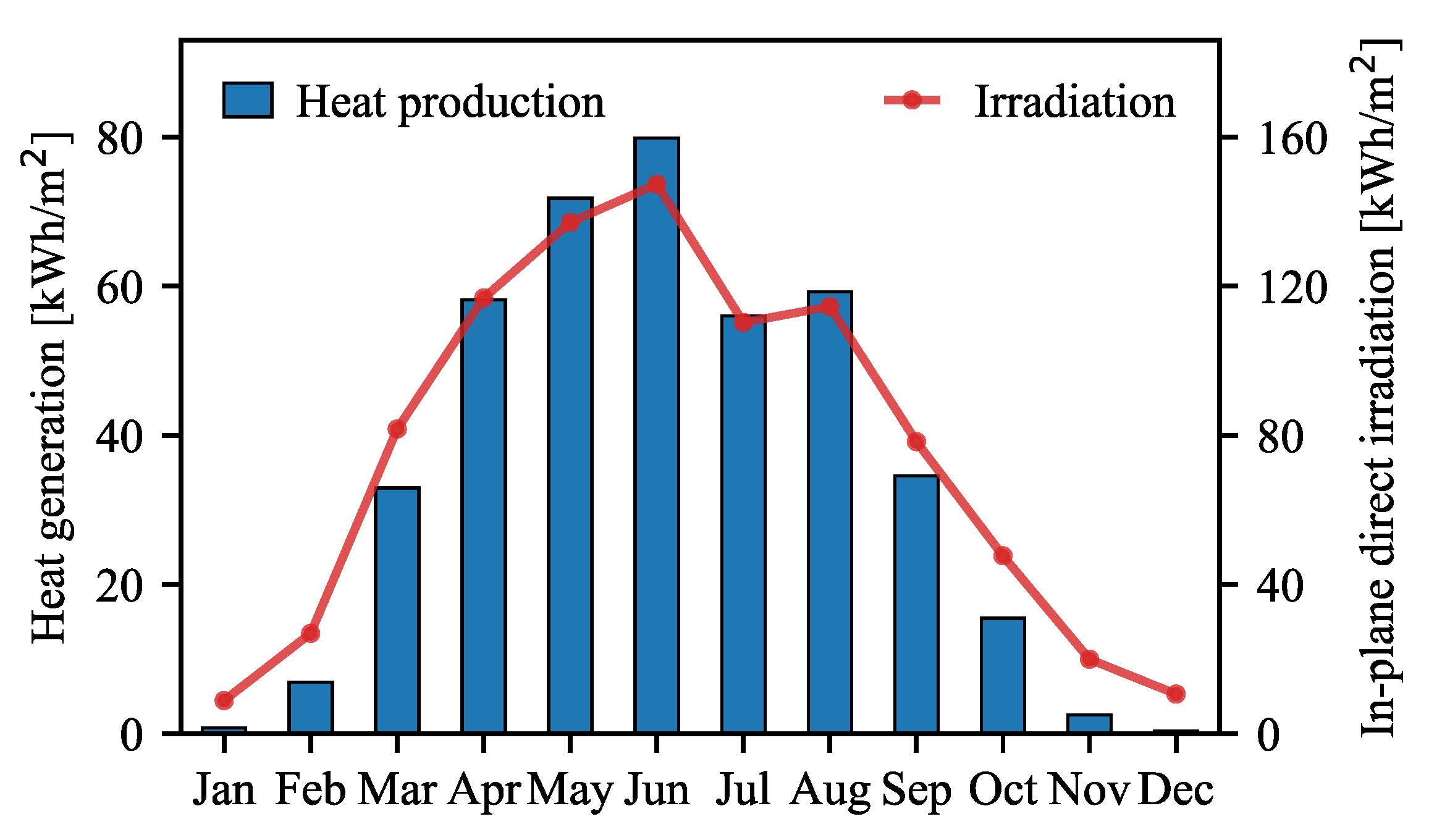
The monthly heat generation for the annual simulation is shown in Figure 8. Over the year, the solar collector field supplied 11.4 GWh to the district heating network, corresponding to 422 kWh/m${}^2$. Based on Figure 8, it is evident that the conversion ratio is much higher in the summer than in the winter. The conversion ratio is defined as the ratio of heat produced (blue bars) to the unshaded in-plane direct irradiation (red points). The lower conversion ratio in the winter is partly attributed to the lower sun elevation (resulting in greater incidence angles and more shading) and the lower ambient temperature (resulting in higher heat losses). Conversely, a higher irradiance level is associated with a higher conversion ratio, as the energy required to heat the system is a smaller proportion of the total daily heat generation.

In comparison, flat-plate collector fields in the region generated 450 kWh/m${}^2$ on average during the period 2012 to 2016 [23]. While the yield of the flat-plate collector fields was slightly higher than the Brønderslev parabolic trough collector field, it is important to note that the heat generated by the parabolic trough collectors was at a much higher temperature. However, such high temperatures are not necessary for direct district heating, and particularly with the general trend of decreasing district heating temperature (low-temperature district heating), the advantage of flat-plate collectors will increase. Thus, PTC fields are better suited for combined heat and power where high-temperature heat is required rather than direct district heating generation. Future research should focus on integrating concentrating collectors with medium- and high-temperature processes, e.g., process heat and combined heat and power. Additionally, if concentrating collectors are to be used for direct district heat generation, research and development should aim at significantly reducing the collector manufacturing costs.

4.4. Sensitivity Results

While the annual simulation was based on the actual solar field configuration, the field layout will surely differ for other systems. For example, the row distance is often dictated by the local land costs, as increasing the row distance reduces shading but comes at the expense of increased land usage. The selection of the tracking axis orientation is often more practical, with the aim of utilizing the available land area as efficiently as possible (restricted by its shape) without excessively compromising the thermal performance. This was also the case for the solar collector field in Brønderslev, which is oriented 29.9° east of north, to match the orientation of the available plot of land. As the row spacing and tracking axis orientation are often selected such that the levelized cost of heat is minimized, it is of great interest to elucidate how changing these parameters affects thermal performance and what annual energy generation can be expected from other systems.

To aid in this decision making, the annual performance as a function of row spacing and axis azimuth orientation is shown as a heat map in Figure 9. Apart from changes to the two parameters, the investigated systems have the same specifications as the solar field in Brønderslev, previously described in Section 3.2. As expected, Figure 9 shows a clear trend of increasing heat generation with increasing row spacing. The reduction in heat generation due to shading is especially pronounced for row spacings shorter than 13 m. In comparison, the variation in heat generation due to the axis azimuth for a fixed row spacing is much less pronounced. The figure also clearly shows that a north–south axis orientation (0° or 180°) is optimal, and an east–west axis orientation (90°) is the least favorable.

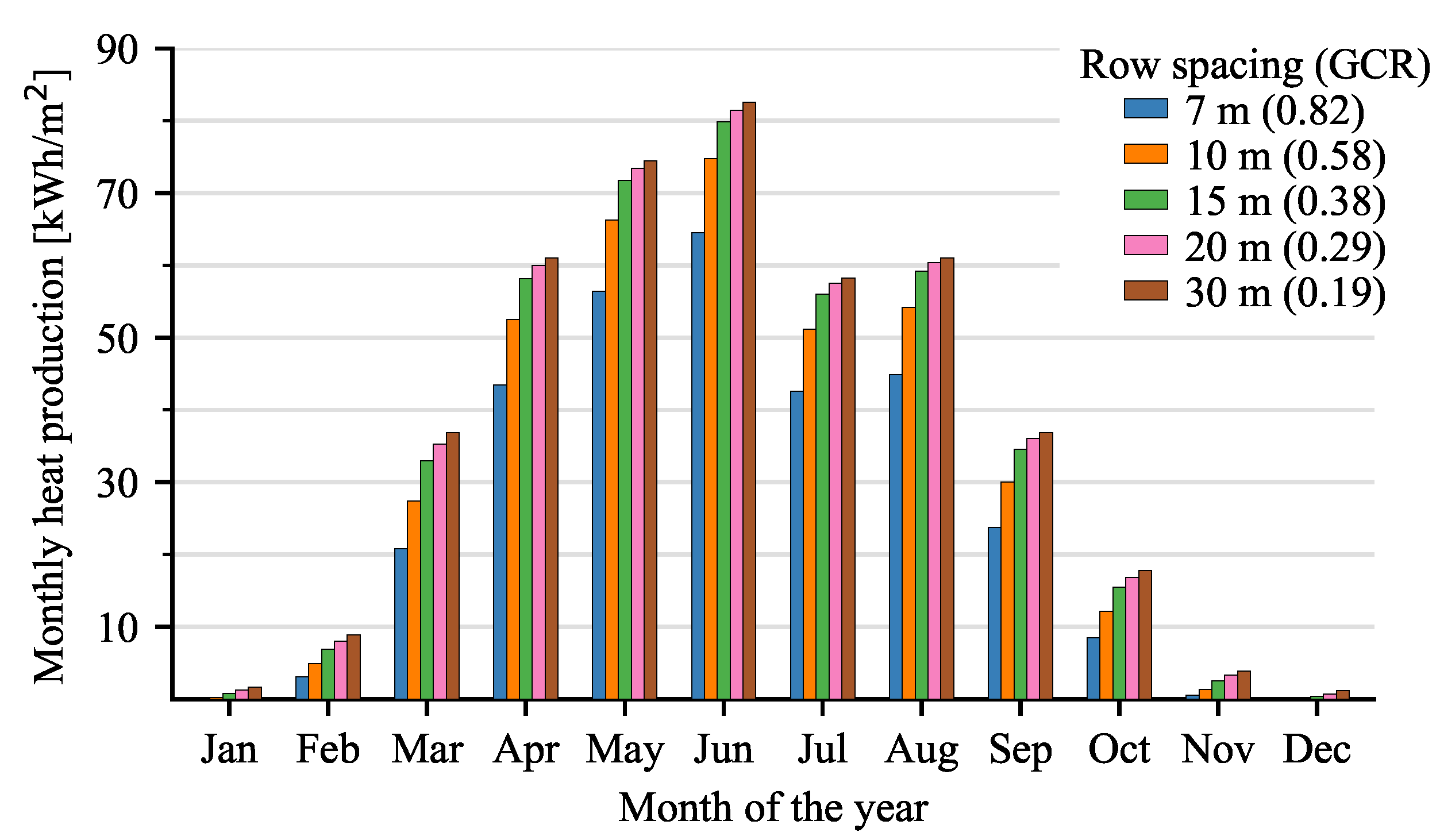
To investigate the impact of row spacing in more detail, the monthly heat production for five different collector distances is shown in Figure 10. The figure shows a heat gain of 6% when doubling the row spacing from 15 to 30 m. In comparison, there is a much larger gain (36%) when the row spacing is increased from 7 to 15 m. This demonstrates that already with a row spacing of 15 m (GCR = 0.38), the effect of shading is relatively low, and there is only a minor gain to be had by increasing the row spacing above 15 m. The economical optimum row spacing is, therefore, expected to be in the range of 11 to 16 m, depending on land costs.

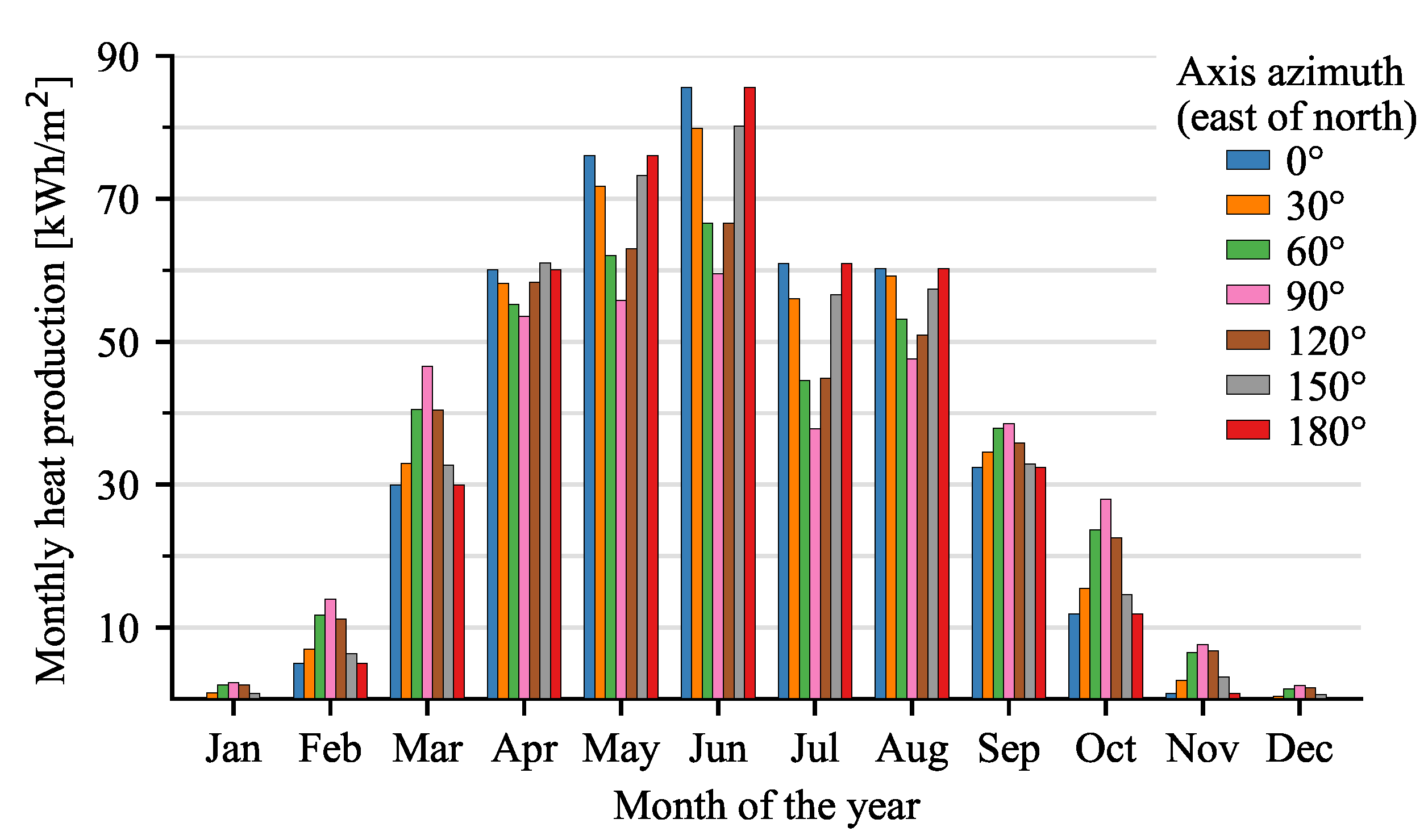
Furthermore, Figure 11 shows the monthly heat production for different axis azimuth orientations. This figure validates the finding of other authors; that the maximum annual energy output in Denmark occurs for a north–south orientation (0° or 180°). However, while this is valid on an annual basis, this is not the case for each month. For example, from September to March, an east–west tracking axis (90°) is preferred due to the lower solar elevation during this time of year. Thus, as the heat demand is higher in winter, it may be preferred to choose an orientation that better matches the demand profile and not the orientation that results in the highest energy yield.

To summarize, the sensitivity simulations showed that the thermal performance of the collector field increased with increasing row spaces, though with limited effect for row spacings greater than 15 m (ground cover ratio of 0.38). Additionally, it was found that the optimal tracking axis orientation was north–south, from which the actual Brønderslev solar field deviates by almost 30°. As a demonstration of the usefulness of the presented results, they can be used to quantify the penalty of a suboptimal tracking axis on an annual basis. The detailed results could also be used to select the tracking axis to achieve a better match to the heat demand if desired. For the Brønderslev plant, the annual output was estimated to be 1% lower than if the optimal tracking axis had been selected. In contrast, the difference between the optimum (0°) and the worst-case orientation (90°) was 7.6%.

Ultimately, the choice of configuration parameters is an economic decision that depends on the local land prices and the available land geometry. Thus, when building new plants, the validated simulation model should be used in conjunction with cost estimates to optimize the plant economy. For example, while the chosen row spacing for the actual Brønderslev solar collector field was found to be a good trade-off between shading and land use, it was not optimized in terms of plant economy. When building a new plant, the authors recommend that all configuration parameters be considered in a thermo-economic simulation study to achieve the lowest levelized cost of heat.

5. Conclusions

In this study, the Brønderslev solar collector field was characterized using the QDT method, and the obtained coefficients were compared to values from the literature. The peak efficiency was found to be 72.7%, which is slightly lower than earlier studies of the same system, suggesting mild soiling conditions. The heat loss and thermal capacity coefficients were more than twice as high compared to a single collector, as the derived coefficients include the effects of the field piping.

Additionally, a TRNSYS model of the solar field integration with the district heating network was developed and validated by comparison against measurements. The model was found to be in close agreement with measured values. The annual simulation showed the field capable of supplying 422 kWh/m${}^2$ per year, with a large seasonal variation. Furthermore, the model was used to study the impact of changing the row spacing and field orientation on the annual energy yield. It was found that increasing the row spacing beyond 15 m (GCR = 0.38) only resulted in small energy gains. It was further shown that an energy yield of more than 7% could be gained by choosing the optimal azimuth (north–south) compared to the worst-case scenario (east–west).

References

1. Perez-Mora, N.; Bava, F.; Andersen, M.; Bales, C.; Lennermo, G.; Nielsen, C.; Furbo, S.; Martínez-Moll, V. Solar district heating and cooling: A review. Int. J. Energy Res. 2018, 42, 1419–1441. [Google Scholar] [CrossRef]
2. Tschopp, D.; Tian, Z.; Berberich, M.; Fan, J.; Perers, B.; Furbo, S. Large-scale solar thermal systems in leading countries: A review and comparative study of Denmark, China, Germany and Austria. Appl. Energy 2020, 270, 114997. [Google Scholar] [CrossRef]
3. SHC IEA. Technology Position Paper–Integration of Large-Scale Solar Heating and Cooling Systems into District Heating and Cooling Networks; IEA Solar Heating and Cooling Technology Collaboration Programme: Cedar, MI, USA, 2021. [Google Scholar]
4. Karlsson, B.; Hultmark, G. Superiority of Flat Plate Collectors in Solar District Heating. In Intersol 85: Proceedings of the Ninth Biennial Congress of the International Solar Energy Society; Pergamon Press: Oxford, UK, 1986; Volume 2, pp. 1003–1007. [Google Scholar] [CrossRef]
5. Tian, Z.; Perers, B.; Furbo, S.; Fan, J. Analysis and validation of a quasi-dynamic model for a solar collector field with flat plate collectors and parabolic trough collectors in series for district heating. Energy 2018, 142, 130–138. [Google Scholar] [CrossRef] [Green Version]
6. Moya, E.Z. Chapter 7—Parabolic-trough concentrating solar power systems. In Concentrating Solar Power Technology, 2nd ed.; Lovegrove, K., Stein, W., Eds.; Woodhead Publishing Series in Energy; Woodhead Publishing: Sawston, UK, 2021; pp. 219–266. [Google Scholar] [CrossRef]
7. Jebasingh, V.K.; Herbert, G.M. A review of solar parabolic trough collector. Renew. Sustain. Energy Rev. 2016, 54, 1085–1091. [Google Scholar] [CrossRef]
8. Perers, B.; Sørensen, P.A.; Kvist, P.; Neergaard, T.B.; Jensen, J.R. A CSP Plant Combined with Biomass CHP Using Orc-Technology in Brønderslev Denmark. In Proceedings of the EuroSun 2016, Palma de Mallorca, Spain, 11–14 October 2016; pp. 1–7. [Google Scholar] [CrossRef]
9. Sallaberry, F.; Tian, Z.; Perers, B.; Furbo, S.; Zourellis, A.; Rothmann, J.H. On-site parabolic-trough collector characterization in solar district heating plant under quasi-dynamic conditions. In AIP Conference Proceedings; American Institute of Physics: Melville, NY, USA, 2019; Volume 2126. [Google Scholar] [CrossRef]
10. Zourellis, A.; Perers, B.; Donneborg, J.; Matoricz, J. Optimizing Efficiency of Biomass—Fired Organic Rankine Cycle with Concentrated Solar Power in Denmark. Energy Procedia 2018, 149, 420–426. [Google Scholar] [CrossRef]
11. Jensen, A.R.; Sifnaios, I.; Caringal, G.P.; Furbo, S.; Dragsted, J. Thermal performance assessment of the world’s first solar thermal Fresnel lens collector field. Sol. Energy 2022, 237, 447–455. [Google Scholar] [CrossRef]
12. Epp, B. Second Winter for 75,000 m² SDH Heating System in Inner Mongolia. 2018. Available online: https://solarthermalworld.org/news/second-winter-75000-m2-sdh-heating-system-inner-mongolia/ (accessed on 2 March 2022).
13. Epp, B. Construction of Largest Swedish SDH Plant with Parabolics. 2020. Available online: https://solarthermalworld.org/news/construction-largest-swedish-sdh-plant-parabolics/ (accessed on 2 March 2022).
14. Vitupier, Y. Helioclim Livre la Plus Grande Centrale Solaire à Concentration de France Pour L’alimentation D’un réseau de Chaleur. 2018. Available online: http://www.helioclim.fr/blog/2018/01/17/helioclim-livre-la-plus-grande-centrale-solaire-a-concentration-de-france-pour-lalimentation-dun-reseau-de-chaleur/ (accessed on 2 March 2022).
15. Tian, Z.; Perers, B.; Furbo, S.; Fan, J. Thermo-economic optimization of a hybrid solar district heating plant with flat plate collectors and parabolic trough collectors in series. Energy Convers. Manag. 2018, 165, 92–101. [Google Scholar] [CrossRef] [Green Version]
16. ISO 9806:2017; Solar Energy—Solar Thermal Collectors—Test Methods. International Organization for Standardization: Geneva, Switzerland, 2017.
17. IEC 62862 Part 3-2; Systems and Components—General Requirements and Test Methods for Large-Size Parabolic-Trough Collectors. IEC: Brussels, Belgium, 2018.
18. Valenzuela, L.; López-Martín, R.; Zarza, E. Optical and thermal performance of large-size parabolic-trough solar collectors from outdoor experiments: A test method and a case study. Energy 2014, 70, 456–464. [Google Scholar] [CrossRef]
19. Klein, S.E.A. TRNSYS 18 a TRaNsient SYstem Simulation Program—Volume 4: Mathematical Reference; Technical Report; Solar Energy Laboratory, University of Wisconsin-Madison: Madison, WI, USA, 2017. [Google Scholar]
20. Wang, P.R.; Scharling, M.; Nielsen, K.P. Technical Report 12-17: 2001–2010 Design Reference Year for Denmark; Technical Report; Danish Meteorological Institute: Copenhagen, Denmark, 2012. [Google Scholar]
21. Perers, B. Verification of High Temperature Performance for the 0.8 MW CSP Test Plant at Brønderslev; Technical Report; Department of Civil Engineering, Technical University of Denmark: Kgs. Lyngby, Denmark, 2015. [Google Scholar]
22. Sallaberry, F.; Valenzuela, L.; Palacin, L.G. On-site parabolic-trough collector testing in solar thermal power plants: Experimental validation of a new approach developed for the IEC 62862-3-2 standard. Sol. Energy 2017, 155, 398–409. [Google Scholar] [CrossRef]
23. Furbo, S.; Dragsted, J.; Perers, B.; Andersen, E.; Bava, F.; Nielsen, K.P. Yearly thermal performances of solar heating plants in Denmark – Measured and calculated. Sol. Energy 2018, 159, 186–196. [Google Scholar] [CrossRef] [Green Version]
Figure 1. Locations of active solar heating plants in Denmark.
Solar 02 00013 g001
Figure 2. Aerial view of the Brønderslev hybrid power plant. Pipes to the solar field are marked with blue, and the return pipes are marked red. Image source: the Danish Agency for Data Supply and Efficiency.
Solar 02 00013 g002
Figure 3. Simplified schematic of the interconnection of the solar collector field and the district heating system.
Solar 02 00013 g003
Figure 4. TRNSYS simulation model (annual) of the Brønderslev concentrating solar collector field and integration with the district heating network.
Solar 02 00013 g004
Figure 5. Visualization of the modeled useful heat production and losses for a clear sky day. For simplicity, the effect of thermal capacity is not shown.
Solar 02 00013 g005
Figure 6. Comparison of measured and modeled values for five days in May 2020.
Solar 02 00013 g006
Figure 7. Comparison of modeled and measured hourly average heat output from the solar collector field for the validation period.
Solar 02 00013 g007
Figure 8. Monthly heat generation and in-plane direct irradiation.
Solar 02 00013 g008
Figure 9. Heat map of the annual heat generation of the solar collector field as a function of axis azimuth orientation and row spacing. The black circle represents the configuration of the Brønderslev solar collector field.
Solar 02 00013 g009
Figure 10. Monthly solar heat production for different row spacings. Values are based on an axis azimuth of 30°. Ground coverage ratio (GCR) is shown in the legend for reference.
Solar 02 00013 g010
Figure 11. Monthly solar heat production for different axis azimuth orientations. Values are based on a row spacing of 15 m.
Solar 02 00013 g011