Picture Hesitant Fuzzy Clustering Based on Generalized Picture Hesitant Fuzzy Distance Measures

Abstract

Certain scholars have generalized the theory of fuzzy set, but the theory of picture hesitant fuzzy set (PHFS) has received massive attention from distinguished scholars. PHFS is the combination of picture fuzzy set (PFS) and hesitant fuzzy set (HFS) to cope with awkward and complicated information in real-life issues. The well-known characteristic of PHFS is that the sum of the maximum of the membership, abstinence, and non-membership degree is limited to the unit interval. This manuscript aims to develop some generalized picture hesitant distance measures (GPHDMs) as a generalization of generalized picture distance measures (GPDMs). The properties of developed distance measures are investigated, and the generalization of developed theory is proved with the help of some remarks and examples. A clustering problem is solved using GPHDMs and the results obtained are explored. Some advantages of the proposed work are discussed, and some concluding remarks based on the summary of the proposed work and as well as future directions, are added.

1. Introduction

Multiple attribute decision making (MADM) procedures, a process for making preference decisions over the available alternatives that are characterized by multiple (usually conflicting) attributes, are useful for improving decision making in a wide range of circumstances. This ranges from professional to managerial to political. In some cases, it is difficult to utilize the fuzzy number, instead of a crisp number, using the MADM technique. As a solution, the theory of fuzzy set (FS) was developed by Zadeh [1]. An FS is defined in terms of a characteristic function describing the membership of an element to a set. Zadeh’s framework was followed extensively by the researchers and some potential work on FS has been completed in fuzzy logic [2], theory and application of fuzzy sets [3], the introduction of fuzzy logic [4], fuzzy switching [5], potential application in fuzzy sets [6], and fuzzy set theory [7]. Generalizing the idea of FS, Atanassov [8] introduced the notion of the intuitionistic fuzzy set (IFS), describing the non-membership degree of an element along with the membership degree of an element [9]. Therefore, in any phenomenon of yes or no type, IFSs played a vital role.

The theory of IFSs could model events containing uncertainty of two types, though there are some scenarios where the framework of IFSs failed to be applied, e.g., the voting event contained four types of situations which are: vote in favor, abstain, vote against, and refused to vote. Such type of event could not be modeled by IFSs, providing a space for a new theory of PFSs developed by Cuong [10]. A PFSs is based on four types of characteristic functions that describe the membership, abstinence, non-membership, and refusal degree. PFSs are an interesting research area as of current, as some potential work on PFSs has been completed in picture fuzzy sets [11], aggregation operators for PFSs [12], and geometric aggregation operators for PFS [13].

In many situations, the theory of FS has failed. For example, when a decision-maker provides information in the form of $\left\{0.5,0.4,0.3\right\}$ for membership grade, the theory of FS has not been able to cope with it. For this, the theory of hesitant fuzzy set (HFS) was developed by Torra [14]. HFS covers only the membership grade in the shape of finite subset of unit interval. An HFS becomes FS if we have the output of characteristic function as a singleton set. For a better understanding of HFSs, we refer to HFS [15], aggregation operators for HFS [16], and intuitionistic hesitant and dual hesitant fuzzy sets [17]. Combining two or more structures enabled us to deal with uncertain events with flexibility. Some generalized structures of HFSs with other fuzzy structures are discussed in [18]. Motivated by the results of bipolar-valued hesitant fuzzy sets [19], operational laws for bipolar HFS [20], and decision-making technique [21], Wang and Li [22] introduced the concept of picture hesitant fuzzy set (PHFS) by generalizing PFSs and HFSs.

In this article, motivated by the work of [23], we developed some GPHDMs and applied them in cluster solving. Cluster analysis has been given great importance in distance measure [24], metric and nonmetric distance measure [25], clustering for IFS [26], and intuitionistic fuzzy clustering [27]. Dealing with clusters having information in the form of hesitant fuzzy numbers (HFNs) provided some flexibility. The distance measures proposed in this manuscript are the generalizations of distance measures of [23]. The GPHDMs have been explained and compared with the existing distance measures for any advantages or shortcomings.

The main idea of this study is taking the some help from the idea of Euclidean distance works effectively when using low-dimensional data, and the magnitude of the vectors is important to be measured. By using the advantages of the measures, the main points of the proposed work are discussed below:

• To develop the GPHDMs as a generalization of GPDMs.
• To initiate the properties of developed distance measures are investigated, and the generalization of developed theory is proved with the help of some remarks and examples.
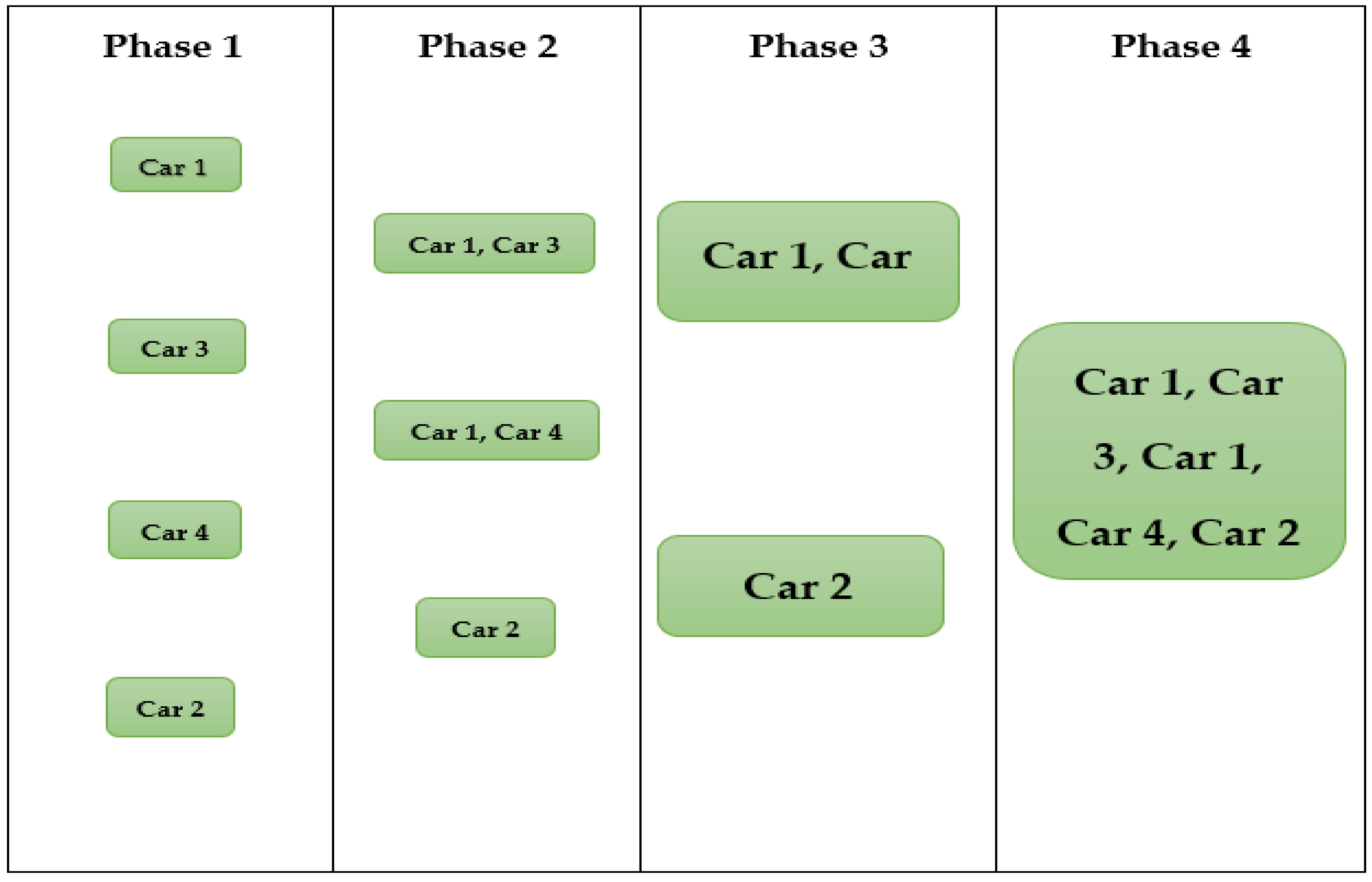
• To explore the clustering problem by using the GPHDMs and the results obtained are explored.
• Some advantages of the proposed work are discussed, and some concluding remarks based on the summary of the proposed work and some future directions are added.

This manuscript is organized as such: In Section 1, a brief history of FSs, IFSs, PFSs, and HFSs is discussed; Section 2 is based on some prerequisite ideas related to IFSs, PFSs, and PHFSs including their distance measures; In Section 3, we developed the picture hesitant distance measures (PHDM), GPHDM, generalized picture hesitant normalized distance measures (GPHNDM), and their generalization is proved; In Section 4, a hierarchal picture hesitant clustering problem is explored. The comparison of proposed and existing work; and Section 5 provided a summary of the manuscript along with some future direction.

2. Literature Review

This section presents concepts related to PFSs, HFSs, and PHFSs. The basic operations of PHFSs are also studied. The theory of IFSs could model events containing uncertainty of two types but there are some scenarios where the framework of IFSs failed to be applied e.g., the voting event contained four types of situations which are vote in favor, abstain, vote against, and refused to vote. Such type of event could not be modeled by IFSs providing a space for a new theory of PFSs was developed by Cuong [10]. The idea of PFS has been discussed below.

Definition 1.

([10]) Let $X$ be a set. Then a PFS is having the shape $Q=\left\{<Ӎ\left(x\right),Ā\left(x\right),\aleph \left(x\right)>:x\in X\right\}$ where $Ӎ:X\to \left[0,1\right]$, $Ā:X\to \left[0,1\right]$ and $\aleph :X\to \left[0,1\right]$ are the degree of membership, abstinence and non-membership degree of $x$ in $Q$ respectively provided that $0\le Ӎ\left(x\right)+Ā\left(x\right)+\aleph \left(x\right)\le 1$. Further, $I\left(x\right)=1-\left(Ӎ\left(x\right)+Ā\left(x\right)+\aleph \left(x\right)\right)$ is termed as refusal degree of $x$ in $X$.

In many situations, the theory of FS has been failed. For instance, when a decision-maker provides information in the form of $\left\{0.5,0.4,0.3\right\}$ for membership grade, then the theory of FS has not been able to cope with it. For managing with such sort of information, the theory of hesitant fuzzy set (HFS) was developed by Torra [14], which defines the membership of an element not only by an element from but by a finite subset of the unit interval.

Definition 2.

([14]) Let $X$ be a set. Then an HFS on $X$ is a mapping $Ӎ$ that gives us few elements of $\left[0,1\right]$ against each $x\in X$. i.e., $H=\{<x,Ӎ\left(x\right)>: Ӎ\left(x\right)$ is a finite subset of $\left[0,1\right] \forall x\in X\}$. Moreover, $Ӎ\left(x\right)$ is called hesitant fuzzy number (HFN).

In some cases, the theory of IFS, PFS, and HFS has been failed. When an intellectual provides information in the shape of such type, which cannot be satisfying the rule of the existing notions like IFS, PFS, and HFS. For this, the theory of PHFS has been proposed, which covers the three grades in the shape of the finite subset of the unit interval.

Definition 3.

([22]) Let $X$ be a set. Then we defined a PHFS as $P=\left\{<\hspace{0.17em}Ӎ,Ā,\aleph >:x\in X\right\}$, such that $Ӎ,Ā,\aleph$ are HFNs denoting the degree of membership, abstinence and non-membership degree of $x$ in $P$ respectively provided that $0\le \sup \left(Ӎ\left(x\right)\right)+\sup \left(Ā\left(x\right)\right)+\sup \left(\aleph \left(x\right)\right)\le 1$. Further, $R\left(x\right)=1-\left(\sup \left(Ӎ\left(x\right)\right)+\sup \left(Ā\left(x\right)\right)+\sup \left(\aleph \left(x\right)\right)\right)$ is termed as refusal degree of $x$ in $X$.

Definition 4.

([22]) Let $P=\left(Ӎ,Ā,\aleph \right)$, $P_1=\left({Ӎ}_1,{Ā}_1,{\aleph }_1\right)$ and $P_2=\left({Ӎ}_2,{Ā}_2,{\aleph }_2\right)$ be the two PHFNs. Then

• $P_1\cup P_2=\left(\max \left({Ӎ}_1,{Ӎ}_2\right),\min \left({Ā}_1,{Ā}_2\right),\min \left({\aleph }_1,{\aleph }_2\right)\right)$;
• $P_1\cap P_2=\left(\min \left({Ӎ}_1,{Ӎ}_2\right),\min \left({Ā}_1,{Ā}_2\right),\max \left({\aleph }_1,{\aleph }_2\right)\right)$
• $P^C=\left(\aleph ,Ā,Ӎ\right)$.

3. Methodology of Development

In this section, we proposed the concept of PHDM, PHNDM, GPHDM and discussed the Hamming and Euclidean distance along with their properties. The defined concepts are supported with an example. Moreover, in our study, we denote the set of all PHFS on universal set $X$ by $PHFӍ\left(X\right)$.

Definition 5.

For$P,Q\in PHFS\left(X\right)$. The PHDM is denoted and defined as:

$$d_{phdᶆ}\left(P,Q\right)={\displaystyle \sum }_{ɉ=1}^{ᶆ}\left(\frac{1}{3z_{x_{ɉ}}}{\displaystyle \sum }_{ᶖ=1}^{z_{x_{ɉ}}}\left(\begin{array}{c}\left|{Ӎ}_P{}^{ȏ(ᶖ)}\left(x_{ɉ}\right)-{Ӎ}_Q{}^{ȏ(ᶖ)}\left(x_{ɉ}\right)\right|+\\ \left|{Ā}_P{}^{ȏ(ᶖ)}\left(x_{ɉ}\right)-{Ā}_Q{}^{ȏ(ᶖ)}\left(x_{ɉ}\right)\right|+\\ \left|{\aleph }_P{}^{ȏ(ᶖ)}\left(x_{ɉ}\right)-{\aleph }_Q{}^{ȏ(ᶖ)}\left(x_{ɉ}\right)\right|\end{array}\right)\right)$$

(1)

The following properties hold for $d_{phdᶆ}\left(P,Q\right)$.

• $0\le d_{phdᶆ}\left(P,Q\right)\le 1$;
• $d_{phdᶆ}\left(P,Q\right)=0⟺P=Q$;
• $d_{phdᶆ}\left(P,Q\right)=d_{phdᶆ}\left(Q,P\right)$;
• $d_{phdᶆ}\left(P,Q\right)+d_{phdᶆ}\left(Q,C\right)\ge d_{phdᶆ}\left(P,C\right)$.

where $z_{x_{ɉ}}$ denote the length of HFN involved in the PHFS.

Definition 6.

For$P,Q\in PHFS\left(X\right)$. The picture hesitant normalized distance measures (PHNDM) is denoted and defined as:

$$d_{phndᶆ}\left(P,Q\right)=\frac{1}{ᶆ}{\displaystyle \sum }_{ɉ=1}^{ᶆ}\left(\frac{1}{3z_{x_{ɉ}}}{\displaystyle \sum }_{ᶖ=1}^{z_{x_{ɉ}}}\left(\begin{array}{c}\left|{Ӎ}_P{}^{ȏ(ᶖ)}\left(x_{ɉ}\right)-{Ӎ}_Q{}^{ȏ(ᶖ)}\left(x_{ɉ}\right)\right|+\\ \left|{Ā}_P{}^{ȏ(ᶖ)}\left(x_{ɉ}\right)-{Ā}_Q{}^{ȏ(ᶖ)}\left(x_{ɉ}\right)\right|+\\ \left|{\aleph }_P{}^{ȏ(ᶖ)}\left(x_{ɉ}\right)-{\aleph }_Q{}^{ȏ(ᶖ)}\left(x_{ɉ}\right)\right|\end{array}\right)\right)$$

(2)

The following properties hold for $d_{phndᶆ}\left(P,Q\right)$.

• $0\le d_{phndᶆ}\left(P,Q\right)\le 1$
• $d_{phndᶆ}\left(P,Q\right)=0⟺P=Q$
• $d_{phndᶆ}\left(P,Q\right)=d_{phndᶆ}\left(Q,P\right)$
• $d_{phndᶆ}\left(P,Q\right)+d_{phndᶆ}\left(Q,C\right)\ge d_{phndᶆ}\left(P,C\right)$

Definition 7.

For$P,Q\in PHFS\left(X\right)$. Then the GPHDM is denoted and defined as:

$$d_{gphdᶆ}\left(P,Q\right)={\left({\displaystyle \sum }_{ɉ=1}^{ᶆ}\left(\frac{1}{3z_{x_{ɉ}}}{\displaystyle \sum }_{ᶖ=1}^{z_{x_{ɉ}}}\left(\begin{array}{c}{\left|{Ӎ}_P{}^{ȏ(ᶖ)}\left(x_{ɉ}\right)-{Ӎ}_Q{}^{ȏ(ᶖ)}\left(x_{ɉ}\right)\right|}^{\gimel }+\\ {\left|{Ā}_P{}^{ȏ(ᶖ)}\left(x_{ɉ}\right)-{Ā}_Q{}^{ȏ(ᶖ)}\left(x_{ɉ}\right)\right|}^{\gimel }+\\ {\left|{\aleph }_P{}^{ȏ(ᶖ)}\left(x_{ɉ}\right)-{\aleph }_Q{}^{ȏ(ᶖ)}\left(x_{ɉ}\right)\right|}^{\gimel }\end{array}\right)\right)\right)}^{\frac{1}{\gimel }}$$

(3)

The following properties hold for $d_{gphdᶆ}\left(P,Q\right)$.

• $0\le d_{gphdᶆ}\left( P,Q\right)\le 1$;
• $d_{gphdᶆ}\left(P,Q\right)=0⟺P=Q$;
• $d_{gphdᶆ}\left(P,Q\right)=d_{gphdᶆ}\left(Q,P\right)$;
• ${\mathrm{d}}_{\mathrm{g}\mathrm{p}\mathrm{h}\mathrm{d}\mathrm{m}}\left(\mathrm{A}\hspace{0.17em}\mathrm{B}\right)+{\mathrm{d}}_{\mathrm{g}\mathrm{p}\mathrm{h}\mathrm{d}\mathrm{m}}\left(\mathrm{B},\mathrm{C}\right)\ge {\mathrm{d}}_{\mathrm{g}\mathrm{p}\mathrm{h}\mathrm{d}\mathrm{m}}\left(\mathrm{A}\hspace{0.17em}\mathrm{C}\right)$.

Definition 8.

For$P,Q\in PHFӍ\left(X\right)$. The GPHNDM is denoted and defined as:

$$d_{gphndᶆ}\left(P,Q\right)={\left(\frac{1}{ᶆ}{\displaystyle \sum }_{ɉ=1}^{ᶆ}\left(\frac{1}{3z_{x_{ɉ}}}{\displaystyle \sum }_{ᶖ=1}^{z_{x_{ɉ}}}\left(\begin{array}{c}{\left|{Ӎ}_P{}^{ȏ(ᶖ)}\left(x_{ɉ}\right)-{Ӎ}_Q{}^{ȏ(ᶖ)}\left(x_{ɉ}\right)\right|}^{\gimel }+\\ {\left|{Ā}_P{}^{ȏ(ᶖ)}\left(x_{ɉ}\right)-{Ā}_Q{}^{ȏ(ᶖ)}\left(x_{ɉ}\right)\right|}^{\gimel }+\\ {\left|{\aleph }_P{}^{ȏ(ᶖ)}\left(x_{ɉ}\right)-{\aleph }_Q{}^{ȏ(ᶖ)}\left(x_{ɉ}\right)\right|}^{\gimel }\end{array}\right)\right)\right)}^{\frac{1}{\gimel }}$$

(4)

The following properties hold for $d_{gphndᶆ}\left(P,Q\right)$.

• $0\le d_{gphndᶆ}\left(P,Q\right)\le 1$
• $d_{gphndᶆ}\left(P,Q\right)=0⟺P=Q$
• $d_{gphndᶆ}\left(P,Q\right)=d_{gphndᶆ}\left(Q,P\right)$
• ${\mathrm{d}}_{\mathrm{g}\mathrm{p}\mathrm{h}\mathrm{n}\mathrm{d}\mathrm{m}}\left(\mathrm{A}\hspace{0.17em}\mathrm{B}\right)+{\mathrm{d}}_{\mathrm{g}\mathrm{p}\mathrm{h}\mathrm{n}\mathrm{d}\mathrm{m}}\left(\mathrm{B},\mathrm{C}\right)\ge {\mathrm{d}}_{\mathrm{g}\mathrm{p}\mathrm{h}\mathrm{n}\mathrm{d}\mathrm{m}}\left(\mathrm{A}\hspace{0.17em}\mathrm{C}\right)$

Remark 1.

If we take$\gimel =1$. Then the Equations (3) and (4) were reduced to generalized picture hesitant Hamming distance measure (GPHHDM) and generalized picture hesitant normalized Hamming distance measure (GPHNHDM) similarly if we take$\gimel =2$. Then the Equations (3) and (4) were reduced to generalized picture hesitant Euclidean distance measure (GPHEDM) and generalized picture hesitant normalized Euclidean distance measure (GPHNEDM). If we considered the abstinence degree equal to zero. Then Equations (1)–(4) holds for IFSs.

Theorem 1.

For$P,Q\in PHFS\left(X\right)$. The following function is a GPHDM.

$$d^1{}_{gphdᶆ}\left(P,Q\right)=\frac{{\left(\frac{1}{z}{{\displaystyle \sum }}_{ɉ=1}^z\left(\begin{array}{c}\frac{△{Ӎ}_{ɉ}{}^{\propto }+△{Ā}_{ɉ}{}^{\propto }+△{\aleph }_{ɉ}{}^{\propto }}{3}+\\ \max \left(△{Ӎ}_{ɉ}{}^{\propto },△{Ā}_{ɉ}{}^{\propto },△{\aleph }_{ɉ}{}^{\propto }\right)\end{array}\right)\right)}^{\frac{1}{\propto }}}{\left(\begin{array}{c}{\left(\frac{1}{z}{{\displaystyle \sum }}_{ɉ=1}^z\left(\begin{array}{c}\frac{△{Ӎ}_{ɉ}{}^{\propto }+△{Ā}_{ɉ}{}^{\propto }+△{\aleph }_{ɉ}{}^{\propto }}{3}+\\ \max \left(△{Ӎ}_{ɉ}{}^{\propto },△{Ā}_{ɉ}{}^{\propto },△{\aleph }_{ɉ}{}^{\propto }\right)\end{array}\right)\right)}^{\frac{1}{\propto }}+\\ {\left(\begin{array}{c}\max \left({\max }_{ɉ}\left({\Psi }_{ɉ}{}^P,{\Psi }_{ɉ}{}^Q\right)\right)+\\ \frac{1}{z}{{\displaystyle \sum }}_{ɉ=1}^z{\left|{\Psi }_{ɉ}{}^P-{\Psi }_{ɉ}{}^Q\right|}^{\propto }\end{array}\right)}^{\frac{1}{\propto }}+1\end{array}\right)}$$

where

$$△{Ӎ}_{ɉ}=\frac{1}{ᶆ}{\displaystyle \sum }_{ɉ=1}^{ᶆ}\left(\frac{1}{z_{x_{ɉ}}}{\displaystyle \sum }_{ᶖ=1}^{z_{x_{ɉ}}}\left|{Ӎ}_P{}^{ȏ(ᶖ)}\left(x_{ɉ}\right)-{Ӎ}_Q{}^{ȏ(ᶖ)}\left(x_{ɉ}\right)\right|\right)$$

$$△{Ā}_{ɉ}=\frac{1}{ᶆ}{\displaystyle \sum }_{ɉ=1}^{ᶆ}\left(\frac{1}{z_{x_{ɉ}}}{\displaystyle \sum }_{ᶖ=1}^{z_{x_{ɉ}}}\left|{Ā}_P{}^{ȏ(ᶖ)}\left(x_{ɉ}\right)-{Ā}_Q{}^{ȏ(ᶖ)}\left(x_{ɉ}\right)\right|\right)$$

$$△{\aleph }_{ɉ}=\frac{1}{Ӎ}{\displaystyle \sum }_{ɉ=1}^{ɉ}\left(\frac{1}{z_{x_{ɉ}}}{\displaystyle \sum }_{ᶖ=1}^{z_{x_{ɉ}}}\left|{\aleph }_P{}^{ȏ(ᶖ)}\left(x_{ɉ}\right)-{\aleph }_Q{}^{ȏ(ᶖ)}\left(x_{ɉ}\right)\right|\right)$$

$${\Psi }_{ɉ}{}^P=\frac{1}{Ӎ}{\displaystyle \sum }_{ɉ=1}^{Ӎ}\left(\underset{ᶖ}{\max }\left|{Ӎ}_P{}^{ȏ(ᶖ)}\left(x_{ɉ}\right)+{Ā}_P{}^{ȏ(ᶖ)}\left(x_{ɉ}\right)+{\aleph }_P{}^{ȏ(ᶖ)}\left(x_{ɉ}\right)\right|\right)$$

$${\Psi }_{ɉ}{}^Q=\frac{1}{ᶆ}{\displaystyle \sum }_{ɉ=1}^{ᶆ}\left(\underset{ɉ}{\max }\left|{Ӎ}_Q{}^{ȏ(ᶖ)}\left(x_{ɉ}\right)+{Ā}_Q{}^{ȏ(ᶖ)}\left(x_{ɉ}\right)+{\aleph }_Q{}^{ȏ(ᶖ)}\left(x_{ɉ}\right)\right|\right)$$

Proof. 

The first three conditions are true by Definition 5. So, we only need to prove condition 4 in Definition (5). For we assume the triplet ($△{Ӎ}_{ɉ}$, $△{Ā}_{ɉ}$, $△{\aleph }_{ɉ}$) and we take $\propto \hspace{0.17em}=1$. Now for $P,Q\in PHFS\left(X\right)$ we denote

$$P{Q}_1={\displaystyle \sum }_{ɉ=1}^z\frac{△{Ӎ}_{ɉ}+△Ā+△{\aleph }_{ɉ}}{3}$$

$$P{Q}_2=\max \left(△{Ӎ}_{ɉ},△{Ā}_{ɉ},△{\aleph }_{ɉ}\right)$$

$$P{Q}_3=\max \left({\max }_{ɉ}\left({\Psi }_{ɉ}{}^P,{\Psi }_{ɉ}{}^Q\right)\right)$$

$$P{Q}_4={\displaystyle \sum }_{ɉ=1}^z\left|{\Psi }_{ɉ}{}^P-{\Psi }_{ɉ}{}^Q\right|$$

We need to show that the following inequality holds.

$$\frac{P{Q}_1+P{Q}_2}{P{Q}_1+P{Q}_2+P{Q}_3+P{Q}_4+1}+\frac{P{C}_1+P{C}_2}{\left(P{C}_1+P{C}_2+P{C}_3+P{C}_4+1\right)}\ge \frac{Q{C}_1+Q{C}_2}{Q{C}_1+Q{C}_2+Q{C}_3+Q{C}_4+1}$$

Using Definition (8), we have

$$\frac{1}{ᶆ}{\displaystyle \sum }_{ɉ=1}^{ᶆ}\left(\frac{1}{z_{x_{ɉ}}}{\displaystyle \sum }_{ᶖ=1}^{z_{x_{ɉ}}}\left|{Ӎ}_P{}^{ȏ(ᶖ)}\left(x_{ɉ}\right)-{Ӎ}_Q{}^{ȏ(ᶖ)}\left(x_{ɉ}\right)\right|\right)+\frac{1}{ᶆ}{\displaystyle \sum }_{ɉ=1}^{ᶆ}\left(\frac{1}{z_{x_{ɉ}}}{\displaystyle \sum }_{ᶖ=1}^{z_{x_{ɉ}}}\left|{Ӎ}_P{}^{ȏ(ᶖ)}\left(x_{ɉ}\right)-{Ӎ}_C{}^{ȏ(ᶖ)}\left(x_{ɉ}\right)\right|\right)\ge \frac{1}{ᶆ}{\displaystyle \sum }_{ɉ=1}^{ᶆ}\left(\frac{1}{z_{x_{ɉ}}}{\displaystyle \sum }_{ᶖ=1}^{z_{x_{ɉ}}}\left|{Ӎ}_Q{}^{ȏ(ᶖ)}\left(x_{ɉ}\right)-{Ӎ}_C{}^{ȏ(ᶖ)}\left(x_{ɉ}\right)\right|\right)$$

$$\frac{1}{ᶆ}{\displaystyle \sum }_{ɉ=1}^{ᶆ}\left(\frac{1}{z_{x_{ɉ}}}{\displaystyle \sum }_{ᶖ=1}^{z_{x_{ɉ}}}\left|{Ā}_P{}^{ȏ(ᶖ)}\left(x_{ɉ}\right)-{Ā}_Q{}^{ȏ(ᶖ)}\left(x_{ɉ}\right)\right|\right)+\frac{1}{ᶆ}{\displaystyle \sum }_{ɉ=1}^{ᶆ}\left(\frac{1}{z_{x_{ɉ}}}{\displaystyle \sum }_{ᶖ=1}^{z_{x_{ɉ}}}\left|{Ā}_P{}^{ȏ(ᶖ)}\left(x_{ɉ}\right)-{Ā}_C{}^{ȏ(ᶖ)}\left(x_{ɉ}\right)\right|\right)\ge \frac{1}{ᶆ}{\displaystyle \sum }_{ɉ=1}^{ᶆ}\left(\frac{1}{z_{x_{ɉ}}}{\displaystyle \sum }_{ᶖ=1}^{z_{x_{ɉ}}}\left|{Ā}_Q{}^{ȏ(ᶖ)}\left(x_{ɉ}\right)-{Ā}_C{}^{ȏ(ᶖ)}\left(x_{ɉ}\right)\right|\right)$$

And

$$\frac{1}{ᶆ}{\displaystyle \sum }_{ɉ=1}^{ᶆ}\left(\frac{1}{z_{x_{ɉ}}}{\displaystyle \sum }_{ᶖ=1}^{z_{x_{ɉ}}}\left|{\aleph }_P{}^{ȏ(ᶖ)}\left(x_{ɉ}\right)-{\aleph }_Q{}^{ȏ(ᶖ)}\left(x_{ɉ}\right)\right|\right)+\frac{1}{ᶆ}{\displaystyle \sum }_{ɉ=1}^{ᶆ}\left(\frac{1}{z_{x_{ɉ}}}{\displaystyle \sum }_{ᶖ=1}^{z_{x_{ɉ}}}\left|{\aleph }_P{}^{ȏ(ᶖ)}\left(x_{ɉ}\right)-{\aleph }_C{}^{ȏ(ᶖ)}\left(x_{ɉ}\right)\right|\right)\ge \frac{1}{ᶆ}{\displaystyle \sum }_{ɉ=1}^{ᶆ}\left(\frac{1}{z_{x_{ɉ}}}{\displaystyle \sum }_{ᶖ=1}^{z_{x_{ɉ}}}\left|{\aleph }_Q{}^{ȏ(ᶖ)}\left(x_{ɉ}\right)-{\aleph }_C{}^{ȏ(ᶖ)}\left(x_{ɉ}\right)\right|\right)$$

Then we have

$$P{Q}_1+P{C}_1\ge Q{C}_1 \mathrm{and} P{Q}_2+P{C}_2\ge Q{C}_2$$

Now suppose that

$$\max \left(\begin{array}{c}\frac{1}{ᶆ}{\displaystyle \sum }_{ɉ=1}^{ᶆ}\left(\frac{1}{z_{x_{ɉ}}}{\displaystyle \sum }_{ᶖ=1}^{z_{x_{ɉ}}}\left|{Ӎ}_Q{}^{ȏ(ᶖ)}\left(x_{ɉ}\right)-{Ӎ}_C{}^{ȏ(ᶖ)}\left(x_{ɉ}\right)\right|\right),\\ \frac{1}{ᶆ}{\displaystyle \sum }_{ɉ=1}^{ᶆ}\left(\frac{1}{z_{x_{ɉ}}}{\displaystyle \sum }_{ᶖ=1}^{z_{x_{ɉ}}}\left|{Ā}_Q{}^{ȏ(ᶖ)}\left(x_{ɉ}\right)-{Ā}_C{}^{ȏ(ᶖ)}\left(x_{ɉ}\right)\right|\right),\\ \frac{1}{ᶆ}{\displaystyle \sum }_{ɉ=1}^{ᶆ}\left(\frac{1}{z_{x_{ɉ}}}{\displaystyle \sum }_{ᶖ=1}^{z_{x_{ɉ}}}\left|{\aleph }_Q{}^{ȏ(ᶖ)}\left(x_{ɉ}\right)-{\aleph }_C{}^{ȏ(ᶖ)}\left(x_{ɉ}\right)\right|\right)\end{array}\right)$$

$$=\frac{1}{ᶆ}{\displaystyle \sum }_{ɉ=1}^{ᶆ}\left(\frac{1}{z_{x_{ɉ}}}{\displaystyle \sum }_{ᶖ=1}^{z_{x_{ɉ}}}\left|{Ӎ}_Q{}^{ȏ(ᶖ)}\left(x_{ɉ}\right)-{Ӎ}_C{}^{ȏ(ᶖ)}\left(x_{ɉ}\right)\right|\right)$$

Then

$$\frac{1}{ᶆ}{\displaystyle \sum }_{ɉ=1}^{ᶆ}\left(\frac{1}{z_{x_{ɉ}}}{\displaystyle \sum }_{ᶖ=1}^{z_{x_{ɉ}}}\left|{Ӎ}_Q{}^{ȏ(ᶖ)}\left(x_{ɉ}\right)-{Ӎ}_C{}^{ȏ(ᶖ)}\left(x_{ɉ}\right)\right|\right)$$

$$\le \frac{1}{ᶆ}{\displaystyle \sum }_{ɉ=1}^{ᶆ}\left(\frac{1}{z_{x_{ɉ}}}{\displaystyle \sum }_{ᶖ=1}^{z_{x_{ɉ}}}\left|{Ӎ}_P{}^{ȏ(ᶖ)}\left(x_{ɉ}\right)-{Ӎ}_Q{}^{ȏ(ᶖ)}\left(x_{ɉ}\right)\right|\right)+\frac{1}{ᶆ}{\displaystyle \sum }_{ɉ=1}^{ᶆ}\left(\frac{1}{z_{x_{ɉ}}}{\displaystyle \sum }_{ᶖ=1}^{z_{x_{ɉ}}}\left|{Ӎ}_P{}^{ȏ(ᶖ)}\left(x_{ɉ}\right)-{Ӎ}_Q{}^{ȏ(ᶖ)}\left(x_{ɉ}\right)\right|\right)$$

$$\max \left(\begin{array}{c}\frac{1}{ᶆ}{\displaystyle \sum }_{ɉ=1}^{ᶆ}\left(\frac{1}{z_{x_{ɉ}}}{\displaystyle \sum }_{ᶖ=1}^{z_{x_{ɉ}}}\left|{Ӎ}_P{}^{ȏ(ᶖ)}\left(x_{ɉ}\right)-{Ӎ}_C{}^{ȏ(ᶖ)}\left(x_{ɉ}\right)\right|\right),\\ \frac{1}{ᶆ}{\displaystyle \sum }_{ɉ=1}^{ᶆ}\left(\frac{1}{z_{x_{ɉ}}}{\displaystyle \sum }_{ᶖ=1}^{z_{x_{ɉ}}}\left|{Ā}_P{}^{ȏ(ᶖ)}\left(x_{ɉ}\right)-{Ā}_C{}^{ȏ(ᶖ)}\left(x_{ɉ}\right)\right|\right),\\ \frac{1}{ᶆ}{\displaystyle \sum }_{ɉ=1}^{ᶆ}\left(\frac{1}{z_{x_{ɉ}}}{\displaystyle \sum }_{ᶖ=1}^{z_{x_{ɉ}}}\left|{\aleph }_P{}^{ȏ(ᶖ)}\left(x_{ɉ}\right)-{\aleph }_C{}^{ȏ(ᶖ)}\left(x_{ɉ}\right)\right|\right)\end{array}\right)$$

$$\frac{Q{C}_1+Q{C}_2}{Q{C}_1+Q{C}_2+Q{C}_3+Q{C}_4+1}\le$$

$$\frac{P{Q}_1+P{Q}_2}{ P{Q}_1+P{Q}_2+P{C}_1+P{C}_2+Q{C}_3+Q{C}_4+1}+\frac{P{C}_1+P{C}_2}{\left(P{Q}_1+P{Q}_2+P{C}_1+P{C}_2+Q{C}_3+Q{C}_4+1\right)}$$

(5)

If we assume that

$$\underset{ɉ}{\max }\left({\Psi }_{ɉ}{}^P,{\Psi }_{ɉ}{}^Q,{\Psi }_{ɉ}{}^{ℂ}\right)={\Psi }_{ɉ}{}^Q,$$

$$\underset{ ɉ}{\max }\left({\Psi }_{ɉ}{}^P,{\Psi }_{ɉ}{}^Q,{\Psi }_{ɉ}{}^{ℂ}\right)={\Psi }_{ɉ}{}^{ℂ}$$

Then $Q{ℂ}_3\ge P{Q}_3$. Again if

$$\underset{ɉ}{\max }\left({\Psi }_{ɉ}{}^P,{\Psi }_{ɉ}{}^Q,{\Psi }_{ɉ}{}^{ℂ}\right)={\Psi }_{ɉ}{}^P$$

Then

$$\underset{ɉ}{\max }\left({\Psi }_{ɉ}{}^P,{\Psi }_{ɉ}{}^Q\right)-\underset{ɉ}{\max }\left({\Psi }_{ɉ}{}^Q,{\Psi }_{ɉ}{}^{ℂ}\right)\le \underset{ɉ}{\max }\left({\Psi }_{ɉ}{}^P-{\Psi }_{ɉ}{}^Q,{\Psi }_{ɉ}{}^Q-{\Psi }_{ɉ}{}^{ℂ}\right)$$

$$\le \underset{ɉ}{\max }\left({\Psi }_{ɉ}{}^P-{\Psi }_{ɉ}{}^Q+{\Psi }_{ɉ}{}^Q-{\Psi }_{ɉ}{}^{ℂ}\right)$$

$$=\underset{ɉ}{\max }\left({\Psi }_{ɉ}{}^P-{\Psi }_{ɉ}{}^{ℂ}\right)\le 3P{ℂ}_2$$

$$P{Q}_3-Q{ℂ}_3\le 3P{ℂ}_2$$

Similarly, we have $Q{ℂ}_4\ge P{Q}_4$ or $3P{ℂ}_2-Q{ℂ}_4\ge P{Q}_4$. Thus

$$3\left(P{Q}_1+P{Q}_2+P{ℂ}_1+P{ℂ}_2+Q{ℂ}_3+Q{ℂ}_4+1\right)\ge P{Q}_1+P{Q}_2+P{Q}_3+P{Q}_4+1$$

(6)

$$3\left(P{Q}_1+P{Q}_2+P{ℂ}_1+P{ℂ}_2+Q{ℂ}_3+Q{ℂ}_4+1\right)\ge P{ℂ}_1+P{ℂ}_2+P{ℂ}_3+P{ℂ}_4+1$$

(7)

From Equations (5)–(7) we claim that $d^1{}_{gphdᶆ}\left(P,Q\right)$ is a PHDM.

Definition 9.

Let$P_{ᶖ}\in PHFӍ\left(X\right)$. Then the average PHFS of$P_{ᶖ}$is denoted and defined as:

$$PVRG\left(P_{ᶖ}\right)=\{<\begin{array}{c}\frac{1}{ᶆ}{\displaystyle \sum }_{ɉ=1}^{ᶆ}{Ӎ}_{ɉ}{}^{ȏ(ᶖ)}\left(x\right),\frac{1}{ᶆ}{\displaystyle \sum }_{ɉ=1}^{ᶆ}{Ā}_{ɉ}{}^{ȏ(ᶖ)}\left(x\right),\\ \frac{1}{ᶆ}{\displaystyle \sum }_{ɉ=1}^{ᶆ}{\aleph }_{ɉ}{}^{ȏ(ᶖ)}\left(x\right)\end{array}>\}$$

Definition 10.

The picture hesitant distance matrix ($PH\aleph M_T$) of order$n\times n$ of $P_{ᶖ}\in PHFӍ\left(X\right)$ is a matrix whose every element is computed by Definition (4).

4. Applications

This section aims to validate the proposed algorithm in the environment of PHFSs. The proposed algorithm is used in the environment of IFS and PFSs in [22]. We will also be described that the frame of IFS and PFS could not handle the data provided in the form of PHFS.

Algorithm

Step 1: Consider a collection $P_{ᶖ}\in PHFӍ\left(X\right)$ where every $P_{ᶖ}$ represent a unique cluster.

Step 2: Compute a $PH\hspace{0.17em}\aleph M_T$.

Step 3: Based on PHDM, combine two PHFS and use Definition (5) to compute the new centers. Note that in one stage only two clusters should be merged.

Step 4: Step two must be repeated unless the desired number of clusters is achieved.

In last, we are constructing the table of the Guangzhou cars data.

Example 1.

Consider Table 1 consisting of a dataset of cars.

The numerical data for the experiment is shown in Table 1, which presents the numbers of cars, their quality, and quantity. To determine the number of people that are interested in the cars, obtaining information on the quality and advantages of the cars is necessary. Therefore, we take the information on the Guangzhou cars and apply the method of PHFS, following the hierarchical principal component (HPC).

Step 1: We take the collection of cars data which represents the quality of the cars that people are interested in, discussed in Table 1.

Table 1. Original decision matrix.

S. No	Comfort	Price	Fuel
Car 1	$\left(\left\{0.1,0.4\right\},\left\{0.2,0.1\right\},\left\{0.3,0.4\right\}\right)$	$\left(\left\{0.3,0.3\right\},\left\{0.4,0.4\right\},\left\{0.1,0.2\right\}\right)$	$\left(\left\{0.3,0.4\right\},\left\{0.3,0.1\right\},\left\{0.2,0.3\right\}\right)$
Car 2	$\left(\left\{0.2,0.4\right\},\left\{0.3,0.2\right\},\left\{0.2,0.3\right\}\right)$	$\left(\left\{0.4,0.4\right\},\left\{0.5,0.4\right\},\left\{0.1,0.1\right\}\right)$	$\left(\left\{0.2,0.3\right\},\left\{0.3,0.4\right\},\left\{0.1,0.2\right\}\right)$
Car 3	$\left(\left\{0.1,0.3\right\},\left\{0.2,0.1\right\},\left\{0.2,0.3\right\}\right)$	$\left(\left\{0.3,0.2\right\},\left\{0.4,0.3\right\},\left\{0.2,0.1\right\}\right)$	$\left(\left\{0.2,0.5\right\},\left\{0.4,0.3\right\},\left\{0.1,0.0\right\}\right)$
Car 4	$\left(\left\{0.2,0.3\right\},\left\{0.3,0.1\right\},\left\{0.3,0.3\right\}\right)$	$\left(\left\{0.4,0.2\right\},\left\{0.5,0.3\right\},\left\{0.2,0.2\right\}\right)$	$\left(\left\{0.1,0.1\right\},\left\{0.2,0.3\right\},\left\{0.4,0.1\right\}\right)$

Table 1. Original decision matrix.

S. No	Comfort	Price	Fuel
Car 1	$\left(\left\{0.1,0.4\right\},\left\{0.2,0.1\right\},\left\{0.3,0.4\right\}\right)$	$\left(\left\{0.3,0.3\right\},\left\{0.4,0.4\right\},\left\{0.1,0.2\right\}\right)$	$\left(\left\{0.3,0.4\right\},\left\{0.3,0.1\right\},\left\{0.2,0.3\right\}\right)$
Car 2	$\left(\left\{0.2,0.4\right\},\left\{0.3,0.2\right\},\left\{0.2,0.3\right\}\right)$	$\left(\left\{0.4,0.4\right\},\left\{0.5,0.4\right\},\left\{0.1,0.1\right\}\right)$	$\left(\left\{0.2,0.3\right\},\left\{0.3,0.4\right\},\left\{0.1,0.2\right\}\right)$
Car 3	$\left(\left\{0.1,0.3\right\},\left\{0.2,0.1\right\},\left\{0.2,0.3\right\}\right)$	$\left(\left\{0.3,0.2\right\},\left\{0.4,0.3\right\},\left\{0.2,0.1\right\}\right)$	$\left(\left\{0.2,0.5\right\},\left\{0.4,0.3\right\},\left\{0.1,0.0\right\}\right)$
Car 4	$\left(\left\{0.2,0.3\right\},\left\{0.3,0.1\right\},\left\{0.3,0.3\right\}\right)$	$\left(\left\{0.4,0.2\right\},\left\{0.5,0.3\right\},\left\{0.2,0.2\right\}\right)$	$\left(\left\{0.1,0.1\right\},\left\{0.2,0.3\right\},\left\{0.4,0.1\right\}\right)$

The numerical data is classified using the method [23], as shown in

Table 2. Calculated values by using different types of measures.

D. Table	Comfort	Price	Fuel
Phases 1
Car 1	0.23	0.28	0.27
Car 2	0.27	0.32	0.25
Car 3	0.20	0.25	0.25
Car 4	0.25	0.30	0.20
Phases 2
Car 13	0.2	0.27	0.26
Car 14	0.25	0.29	0.23
Phases 3
Car 1314	0.24	0.25	0.25
Car 2	0.27	0.32	0.25

. During the first phase, the Guangzhou cars data is in the following format:

{Car 1}, {Car 2}, {Car 3}, {Car 4}.

The set of numerical data is classified by phase and score function in this table [23].

Step 2: using the step 1 data to compute $PH\hspace{0.17em}\aleph M_t$

$$PH\hspace{0.17em}\aleph M_t=\left(\begin{array}{c}0\\ \begin{array}{c}0.38\\ \begin{array}{c}0.35\\ 0.52\end{array}\end{array}\end{array} \begin{array}{c}0.38\\ \begin{array}{c}0\\ \begin{array}{c}0.37\\ 0.4\end{array}\end{array}\end{array} \begin{array}{c}0.35\\ \begin{array}{c}0.37\\ \begin{array}{c}0\\ 0.47\end{array}\end{array}\end{array} \begin{array}{c}0.52\\ \begin{array}{c}0.4\\ \begin{array}{c}0.47\\ 0\end{array}\end{array}\end{array}\right)$$

In this stage, the minimum value is $d\left(P_1,P_3\right)=0.35$ and the maximum value is $d\left(P_1,P_4\right)=0.52$, then $P_1$ and $P_3$ are combined in the next stage and similarly,$P_1$ and $P_4$ are merged in the next stage. So the results of phase two are above and using the concepts we make the other phases numerically data.

Step 3: Based on PHDM, combine two PHFS and use Definition (5) to compute the new centers are discussed in the shape of

Table 3. Again merged and phases-wise classification.

D. T	Comfort	Price	Fuel
Car 13	$\left(\left\{0.1,0.35\right\},\left\{0.2,0.1\right\},\left\{0.25,0.35\right\}\right)$	$\left(\left\{0.3,0.25\right\},\left\{0.4,0.35\right\},\left\{0.15,0.15\right\}\right)$	$\left(\left\{0.25,0.45\right\},\left\{0.35,0.2\right\},\left\{0.15,0.15\right\}\right)$
Car 14	$\left(\left\{0.15,0.35\right\},\left\{0.25,0.1\right\},\left\{0.3,0.35\right\}\right)$	$\left(\left\{0.35,0.25\right\},\left\{0.45,0.35\right\},\left\{0.15,0.2\right\}\right)$	$\left(\left\{0.2,0.25\right\},\left\{0.25,0.27\right\},\left\{0.3,0.2\right\}\right)$

.

In phase two the Guangzhou cars data is of the form:

{Car 1, Car 3}, {Car 1, Car 4}, {Car 2}.

(8)

Step 4: Repeated step 2 to construct the $PH\hspace{0.17em}\aleph M_t$

$$GPH\hspace{0.17em}\aleph M^2=\left(\begin{array}{ccc}0& 0.24& 0.34\\ 0.24& 0& 0.31\\ 0.34& 0.31& 0\end{array}\right)$$

(9)

Here, the low value is produced by d({Car 1, Car 3}}, {{Car 2, Car 4}) = 0.24 in $GPH\hspace{0.17em}\aleph M^2$. We are constructing the table which represents the summary of all the different phases, described in the above algorithm using the Guangzhou cars data as illustrated in Figure 1.

Step 3: Based on PHDM, combine two PHFS and use the definition (5) to compute the new centers, as discussed in

Table 4. Merged and phase-wise classification.

D. T	Comfort	Price	Fuel
Car 1314	$\left(\left\{0.125,0.35\right\},\left\{0.225,0.1\right\},\left\{0.275,0.35\right\}\right)$	$\left(\left\{0.325,0.25\right\},\left\{0.425,0.35\right\},\left\{0.15,0.175\right\}\right)$	$\left(\left\{0.225,0.35\right\},\left\{0.30,0.235\right\},\left\{0.225,0.175\right\}\right)$

.

Similarly, in the last phases the Guangzhou cars data is of the form:

{Car 1, Car 3, Car 1, Car 4}, {Car 2}.

Step 4: Repeated step 2 to construct the $PH\hspace{0.17em}\aleph M_t$

$$GPH\hspace{0.17em}\aleph M^3=0.303$$

We evaluate all numerical data of the Guangzhou cars and draw the tables for investigation of the three different values of $PH\hspace{0.17em}\aleph M_t$.

Remark 2.

We take all the PHFS in the form of singleton sets, then reduce all concepts into PFS. If we choose to ignore the abstinence degree, it will be converted to IFS. The proposed work is converted to all concepts like PFS, HFS, IHFS, IFS, and FS, which is the modified form of PFS, and its elements are HFS.

The above discussion shows that our proposed work is more effective and more reliable in comparison to existing work.

5. Conclusions

Numerous scholars have employed the theory of PHFS in the environment of different fields. PHFS has received massive attention from different intellectuals due to its shape, where the rule is that the sum of the maximum of the triplet is restricted to the unit interval. The main purpose of this manuscript is discussed below.

• We examined the GPHDM and defined the special cases like GPHHDM and GPHEDM.
• We worked on GPHNDM and defined special cases like GPHNHDM and GPHNEDM.
• We evaluated the application and show whose concepts are assigned the best results in distance measure.
• Finally, we proposed the numerical data table and described their applications with the help of an algorithm.

In upcoming research, we will attempt to employ the theory of T-spherical fuzzy sets [28], Complex spherical fuzzy sets [29], complex T-spherical fuzzy sets [30], and bipolar soft sets [31] in the field of computer science, engineering science, etc., to improve the quality of the research works.

References

1. Zadeh, L.A. Fuzzy sets. Inf. Control 1965, 8, 338–353. [Google Scholar] [CrossRef] [Green Version]
2. Klir, G.; Yuan, B. Fuzzy Sets and Fuzzy Logic; Prentice Hall: Upper Saddle River, NJ, USA, 1995; Volume 4, pp. 1–12. [Google Scholar]
3. Dubois, D.J. Fuzzy Sets and Systems: Theory and Applications; Academic Press: New York, NY, USA; London, England; Toronto, Canada; Sydney, Australia; San Francisco, CA, USA, 1980; Volume 144, pp. 1–8. [Google Scholar]
4. Yager, R.R.; Zadeh, L.A. An Introduction to Fuzzy Logic Applications in Intelligent Systems; Springer Science & Business Media: Wilmersdorf, Berlin, Germany, 2012; Volume 16, pp. 1–9. [Google Scholar]
5. Kandel, A.; Lee, S.C.; Wang, C.Y. Fuzzy switching and automata. IEEE Trans. Syst. Man. Cybern. 1980, 10, 690. [Google Scholar] [CrossRef]
6. Karwowski, W.; Mital, A. Potential applications of fuzzy sets in industrial safety engineering. Fuzzy Sets Syst. 1986, 19, 105–120. [Google Scholar] [CrossRef]
7. Zimmermann, H.J. Applications of fuzzy set theory to mathematical programming. Inf. Sci. 1985, 36, 29–58. [Google Scholar] [CrossRef]
8. Atanassov, K.T. Intuitionistic fuzzy sets. Fuzzy Sets Syst. 1986, 20, 87–96. [Google Scholar] [CrossRef]
9. Burillo, P.J.; Bustince, H. Intuitionistic fuzzy relations (Part I). Mathw. Soft Comput. 1995, 2, 5–38. [Google Scholar]
10. Cuong, B.C. Picture fuzzy sets-First results. Part 1. Semin. Neuro-Fuzzy Syst. Appl. 2013, 4, 1–16. [Google Scholar]
11. Cường, B.C. Picture fuzzy sets. J. Compu. Sci. Cybern. 2014, 30, 409. [Google Scholar] [CrossRef] [Green Version]
12. Garg, H. Some picture fuzzy aggregation operators and their applications to multicriteria decision-making. Arab. J. Sci. Eng. 2017, 42, 5275–5290. [Google Scholar] [CrossRef]
13. Wang, C.; Zhou, X.; Tu, H.; Tao, S. Some geometric aggregation operators based on picture fuzzy sets and their application in multiple attribute decision making. Ital. J. Pure Appl. Math 2017, 37, 477–492. [Google Scholar]
14. Torra, V. Hesitant fuzzy sets. Int. J. Intell. Syst. 2010, 25, 529–539. [Google Scholar] [CrossRef]
15. Torra, V.; Narukawa, Y. On hesitant fuzzy sets and decision. In Proceedings of the 2009 IEEE Inter Conference on Fuzzy Systems, Jeju, Korea, 20–24 August 2009; Volume 1, pp. 1378–1382. [Google Scholar]
16. Xia, M.; Xu, Z. Hesitant fuzzy information aggregation in decision making. Int. J. Approx. Reason. 2011, 52, 395–407. [Google Scholar] [CrossRef] [Green Version]
17. Liu, X.; Ju, Y.; Yang, S. Hesitant intuitionistic fuzzy linguistic aggregation operators and their applications to multiple attribute decision making. J. Int. Fuzzy Syst. 2014, 27, 1187–1201. [Google Scholar]
18. Zhu, B.; Xu, Z.; Xia, M. Dual hesitant fuzzy sets. J. Appl. Math 2012, 1, 1–19. [Google Scholar] [CrossRef]
19. Mahmood, T.; Ullah, K.; Khan, Q. Some Aggregation Operators for Bipolar-Valued Hesitant Fuzzy Information. J. Fund Appl. Sci. 2018, 10, 240–245. [Google Scholar]
20. Mahmood, T.; Ullah, K.; Jan, N.; Deli, I.; Khan, Q. Some Aggregation Operators for Bipolar-Valued Hesitant Fuzzy Information based on Einstein Operational Laws. J. Engine Appl. Sci. 2017, 36, 1–27. [Google Scholar]
21. Ullah, K.; Mahmood, T.; Jan, N.; Broumi, S.; Khan, Q. On bipolar-valued hesitant fuzzy sets and their applications in multi-attribute decision making. Nucleus 2018, 55, 85–93. [Google Scholar]
22. Wang, R.; Li, Y. Picture hesitant fuzzy set and its application to multiple criteria decision-making. Symmetry 2018, 10, 295. [Google Scholar] [CrossRef] [Green Version]
23. Son, L.H. Generalized picture distance measure and applications to picture fuzzy clustering. Appl. Soft Comput. 2016, 46, 284–295. [Google Scholar] [CrossRef]
24. Pandit, S.; Gupta, S. A comparative study on distance measuring approaches for clustering. Int. J. Res. Comput. Sci. 2011, 2, 29–31. [Google Scholar] [CrossRef] [Green Version]
25. Ackermann, M.R.; Blömer, J.; Sohler, C. Clustering for metric and nonmetric distance measures. ACM Trans. Algorithms (TALG) 2010, 6, 59. [Google Scholar] [CrossRef]
26. Pelekis, N.; Iakovidis, D.K.; Kotsifakos, E.E.; Kopanakis, I. Fuzzy clustering of intuitionistic fuzzy data. Int. J. Bus. Intell. Data Min. 2008, 3, 45–65. [Google Scholar] [CrossRef]
27. Son, L.H.; Cuong, B.C.; Lanzi, P.L.; Thong, N.T. A novel intuitionistic fuzzy clustering method for geo-demographic analysis. Expert Syst. Appl. 2012, 39, 9848–9859. [Google Scholar] [CrossRef]
28. Mahmood, T.; Ullah, K.; Khan, Q.; Jan, N. An approach toward decision-making and medical diagnosis problems using the concept of spherical fuzzy sets. Neural Comp. Appl. 2019, 31, 7041–7053. [Google Scholar] [CrossRef]
29. Ali, Z.; Mahmood, T.; Yang, M.S. TOPSIS method based on complex spherical fuzzy sets with Bonferroni mean operators. Mathematics 2020, 8, 1739. [Google Scholar] [CrossRef]
30. Ali, Z.; Mahmood, T.; Yang, M.S. Complex T-spherical fuzzy aggregation operators with application to multi-attribute decision making. Symmetry 2020, 12, 1311. [Google Scholar] [CrossRef]
31. Mahmood, T. A Novel Approach towards Bipolar Soft Sets and Their Applications. J. Math. 2020, 2020, 4690808. [Google Scholar] [CrossRef]
Figure 1. The Guangzhou cars data table represents the four phases.
Knowledge 01 00005 g001