Article

A Novel Method That Is Based on Differential Evolution Suitable for Large-Scale Optimization Problems

by
Glykeria Kyrou
*,
Vasileios Charilogis
and
Ioannis G. Tsoulos
Department of Informatics and Telecommunications, University of Ioannina, 47150 Kostaki Artas, Greece
*
Author to whom correspondence should be addressed.
Foundations 2026, 6(1), 2; https://doi.org/10.3390/foundations6010002
Submission received: 4 December 2025 / Revised: 15 January 2026 / Accepted: 19 January 2026 / Published: 23 January 2026
(This article belongs to the Section Mathematical Sciences)

Abstract

Global optimization represents a fundamental challenge in computer science and engineering, as it aims to identify high-quality solutions to problems spanning from moderate to extremely high dimensionality. The Differential Evolution (DE) algorithm is a population-based algorithm like Genetic Algorithms (GAs) and uses similar operators such as crossover, mutation and selection. The proposed method introduces a set of methodological enhancements designed to increase both the robustness and the computational efficiency of the classical DE framework. Specifically, an adaptive termination criterion is incorporated, enabling early stopping based on statistical measures of convergence and population stagnation. Furthermore, a population sampling strategy based on k-means clustering is employed to enhance exploration and improve the redistribution of individuals in high-dimensional search spaces. This mechanism enables structured population renewal and effectively mitigates premature convergence. The enhanced algorithm was evaluated on standard large-scale numerical optimization benchmarks and compared with established global optimization methods. The experimental results indicate substantial improvements in convergence speed, scalability and solution stability.

1. Introduction

The basic goal of global optimization is to find the global minimum of a continuous multidimensional function and is defined as
x * = arg min x S f ( x )
with S:
S = a 1 , b 1 × a 2 , b 2 × a n , b n
with a i and b i representing lower and upper bounds for each variable, x i .
In recent years many researchers have published important reviews on global optimization. Such methods find application in a wide range of scientific fields, such as mathematics [1], physics [2], chemistry [3], biology [4], medicine [5], agriculture [6] and economics [7]. A particular challenge is the large-scale global optimization (LSGO) problem, where the complexity increases significantly with increasing problem dimensions. Finding efficient and computationally feasible solutions has become particularly difficult, which has led the research community to focus on the development of innovative algorithms. LSGO problems are encountered in a wide range of applications, while their importance was also reflected in the organization of the first global large-scale optimization competition within the framework of the CEC in 2008. Other competitions followed in 2010 [8], 2013 [9] and 2015 [10], attracting the intense interest of the academic community.
To address these challenges, various heuristic and meta-heuristic approaches have been developed. Evolutionary algorithms (EAs) [11] are one of the most effective categories, as they mimic natural selection and genetic evolution to search for best solutions. Due to their adaptability and robustness, EAs can solve difficult optimization problems. Some of the most well-known EAs are DE [12], GAs [13], evolutionary strategies [14], evolutionary programming [15] and multimodal optimization algorithms [16]. Also, methods inspired by Swarm Intelligence [17] such as Particle Swarm Optimization (PSO) [18], Ant Colony Optimization (ACO) [19], Artificial Bee Colony (ABC) Optimization [20], the Firefly Algorithm (FA) [21] and the Bat Algorithm [22], Arithmetic Optimization Algorithm (AOA) [23] are strong alternatives.
DE is one of the most widely used optimization techniques, as it offers high robustness, simplicity and fast convergence. DE is a highly efficient evolutionary algorithm that has gained significant recognition since the late 1990s. DE, originally introduced in 1995 by Storn and Price [24], has proven to be a versatile optimization tool that can be applied in various scientific and engineering fields. It is particularly effective for symmetric optimization problems, as well as for dealing with discontinuous, noisy and dynamic challenges. In physics, it has been used in energy-related problems, including wind power optimization [25]. In chemistry, it has contributed to advances in atmospheric chemistry and the development of high-performance chemical reactors [26]. DE has also had significant implications in health-related areas, such as breast cancer research and medical diagnostics [27]. Despite its effectiveness, classical DE may face additional challenges when applied to high-dimensional and large-scale optimization problems. In such settings, the adaptation of control parameters becomes more demanding, while exploitation efficiency during later stages of the search process may be reduced. Moreover, as problem dimensionality increases, maintaining fast convergence and high solution accuracy can become more difficult. These observations have motivated extensive research efforts toward the development of enhanced DE variants, aiming to improve adaptability, scalability and the balance between exploration and exploitation in large-scale optimization problems.
Recent studies have proposed various strategies to address large-scale optimization challenges, including cooperative coevolution [28], Particle Swarm Optimization [29], a DE approach [30], distributed differential evolution with adaptive resource allocation [31], hybrid swarm-based algorithms combining multiple search mechanisms [32], a self-adaptive Fast Fireworks Algorithm [33], swarm-based methods with learning mechanisms [34] and advanced decomposition techniques such as dual Differential Grouping [35]. These approaches highlight the ongoing research interest in designing efficient and scalable optimization frameworks for large-scale problems.
In this work, a unified and modular DE framework is proposed to improve efficiency, robustness and convergence behavior in large-scale optimization problems. Instead of relying on a single evolutionary strategy or fixed parameter settings, the proposed approach integrates multiple enhancement mechanisms within a single DE framework. These mechanisms are designed to be independently configurable, allowing the algorithm to adapt more effectively to diverse problem characteristics while preserving the fundamental structure of classical DE.
The main contributions of this paper are summarized as follows:
  • A unified and modular DE framework is introduced, integrating multiple control mechanisms within a single optimization scheme, including mutation weighting, parent selection, local refinement activation and termination criteria.
  • A k-means-based population sampling strategy is incorporated to preserve population structure and improve sampling efficiency in high-dimensional search spaces.
  • Alternative mechanisms for computing the differential weight parameter are proposed, incorporating number-based, random and migrant strategies to enhance adaptability in large-scale optimization problems.
  • An optional tournament-based parent selection strategy is employed to improve selection pressure while maintaining population diversity and robustness.
  • A periodic local optimization refinement using deterministic local optimizers, such as BFGS, is integrated to enhance solution accuracy and accelerate convergence without compromising global exploration.
  • A population-based termination criterion is introduced to enable early stopping when convergence stagnation is detected, significantly reducing unnecessary objective function evaluations.
  • The proposed framework is specifically designed for large-scale global optimization problems and aims to achieve a more effective balance between exploration and exploitation compared to classical DE variants.
Although the individual enhancement mechanisms employed in the proposed framework, including adaptive termination strategies, clustering-based population initialization, adaptive differential weight schemes and local optimization techniques, have been previously studied in the literature, their combined integration within a single DE framework is not straightforward. Each mechanism operates in a distinct stage of the evolutionary process and affects different aspects of the search dynamics, such as diversity preservation, convergence behavior and computational efficiency.
The contribution of the present work lies in the systematic and modular coordination of these mechanisms within a unified optimization framework. By enabling controlled interaction between global exploration, adaptive parameter control, local exploitation and termination mechanisms, the proposed approach facilitates synergistic effects that cannot be readily achieved through the isolated application of individual enhancements. This structured integration provides a principled framework for improving robustness and scalability in large-scale global optimization problems.
Importantly, the novelty of the proposed approach lies not in the introduction of new standalone operators but in the principled way these mechanisms are coordinated within a single framework. Each component is explicitly designed to operate in synergy with the others, rather than being applied independently. In particular, structured sampling and adaptive differential weighting jointly influence population diversity and step-size control, while tournament selection ensures that informative population feedback is preserved for adaptive mechanisms to exploit. This coordinated interaction provides a theoretical justification for the combined framework and explains why its behavior cannot be reduced to a simple aggregation of existing techniques.
The remaining parts of this paper are divided as follows: In Section 2 the original DE algorithm, the proposed method and a flowchart with detailed description are presented. In Section 3 of the test functions used in the experiments as well as the related experiments are presented. In Section 4, there is a brief discussion of the results obtained from the experiments. In Section 5 some conclusions and directions for future improvements are discussed.

2. Differential Evolution Algorithm

2.1. The Original Differential Evolution Method

DE is a population-based evolutionary algorithm that has been widely used for continuous optimization problems. The method maintains a population of candidate solutions, which are iteratively evolved through the application of mutation, crossover and selection operators. In each iteration, new candidate solutions are generated by combining information from multiple population members, while selection is performed based on objective function comparisons. The DE procedure begins by defining the population size N P . In order to ensure the feasibility of the classical DE mutation operator, which requires three distinct population members in addition to the target vector, a minimum population size of N P 4 is required. In practice, the population size is often related to the dimensionality of the optimization problem. A commonly adopted guideline in the DE literature is to set N P = 10 n , where n denotes the problem dimension, as this choice has been shown to provide robust performance across a wide range of problems without extensive parameter tuning. We note that alternative formulations relating the population size to the problem dimension have also been proposed in the literature; however, such choices are problem-dependent and do not affect the general applicability of the DE framework. The initial population is generated randomly within the search space and evaluated using the objective function. During each iteration, for every target vector, x i , three distinct population members are randomly selected to construct a mutant vector through a differential mutation operation. This mutant vector is then combined with the target vector using a binomial crossover mechanism, producing a trial vector. If the trial vector achieves an objective function value that is not worse than that of the target vector, it replaces the target vector in the population. The evolutionary process continues until a termination criterion is satisfied, such as reaching a maximum number of iterations or meeting a convergence condition. The algorithm returns the best solution found during the search process. Regarding parameter settings, the crossover probability is set to C R = 0.9 and the differential weight to F = 0.8 , following values commonly adopted in the DE literature [36]. These parameter values have been empirically shown to provide stable performance across a broad range of optimization problems without requiring problem-specific tuning. In this study, all parameters of the original DE algorithm are kept fixed throughout the experimental evaluation in order to ensure a fair and unbiased comparison with the proposed method. For clarity, the full steps of the original DE algorithm are summarized in Algorithm 1.
Algorithm 1 Original Differential Evolution Algorithm
INPUT
- f: objective function
- N P : population size
- C R : Crossover rate
- F: Differential weight
- n: Problem dimension
OUTPUT
- x b e s t
INITIALIZATION
-Generate an initial population of N P candidate solutions x i , i = 1 , , N P , uniformly at random within the search bounds.
-Evaluate the objective function f ( x i ) for all individuals.
-Set x b e s t as the individual with the best objective value.
main pseudocode
01 while stopping criterion is not met do
02   for each individual i , i {1… N P } do
03      Select randomly three agents a , b , c {1… N P }
04      Generate mutant vector u = a j + F × ( b j c j )
05      Select a random index R {1…n}
06      for each dimension j = 1 to n do
07         Generate a random number r i [ 0 , 1 ]
08         if  r j < C R o r j = R then
09            Set y j = u j .
10         else
11            Set y j = x i j .
12         endif
13      endfor
14      if f ( y ) f ( x i )  then
15        Replace x i   w i t h   y
16      endif
17   endfor
18 endwhile
19 return  x b e s t

2.2. The Proposed Differential Evolution Method

The main contribution of the proposed approach is the formulation of a unified and modular DE framework that systematically integrates multiple control mechanisms within a single optimization scheme. Unlike most existing DE variants, which typically modify a single algorithmic component (e.g., mutation strategy or parameter adaptation), the proposed method allows the independent configuration and combined use of several algorithmic mechanisms while preserving the fundamental evolutionary structure of the original DE algorithm. The proposed method extends the classical DE framework by introducing a modular design that incorporates additional control components related to differential weight computation, parent selection, local refinement and termination criteria. This design enables both the independent analysis of each component and their joint exploitation within a single, coherent optimization process, facilitating a systematic investigation of robustness and parameter sensitivity. The main methodological contributions of the proposed framework can be summarized as follows:
  • Alternative mechanisms for differential weight computation.
  • A k-means-based population sampling strategy is incorporated to preserve population structure and improve sampling efficiency in high-dimensional search spaces.
  • Optional tournament-based parent selection strategies.
  • Periodic local refinement using a deterministic local optimizer.
  • A population-based termination criterion.
The algorithm starts with an initialization phase in which a population of N P agents is randomly generated and evaluated using the objective function. Additional control parameters are also initialized in this stage, including the local search rate p l , which determines the frequency of local refinement, the tournament size N t , which controls selection pressure, the maximum number of generations N g , the termination criteria N I and the iteration counter k. During the evolutionary process, different strategies for computing the differential weight F can be employed. These include a constant value and a random mechanism defined as F = 0.5 + 2 r , where r [ 0 , 1 ] , as well as a migrant-based strategy [37]. For each agent, candidate solutions are generated through mutation and crossover operations, followed by a selection step based on objective function comparisons. In addition to the evolutionary operators, a deterministic local search procedure based on the BFGS method [38] may be periodically applied to refine promising solutions. The optimization process proceeds iteratively until a termination condition is satisfied, which may be defined either by a maximum number of generations or by a population-based convergence criterion. By jointly integrating stochastic variation, adaptive differential weight mechanisms and deterministic local refinement within a unified framework, the proposed method aims to improve search efficiency and to achieve a more effective balance between exploration and exploitation. Moreover, the modular structure of the algorithm allows the systematic evaluation of the effect of individual algorithmic components, as demonstrated in the sensitivity analysis presented in Section 3. For clarity, the complete steps of the proposed DE algorithm are summarized in Algorithm 2.
The main steps of the proposed DE algorithm are illustrated in the flowchart presented in Figure 1.
Algorithm 2 Proposed Algorithm
INPUT
- f: objective function
- N P : population size
- N t : tournament size
- N g : maximum number of iterations
- N I : termination criteria
- C R : Crossover rate
- F: Differential weight
- n: Problem dimension
- k: iteration counter
OUTPUT
- x b e s t
INITIALIZATION
-Set as N P the population size (number of agents)
-Create randomly NP agents x i , i = 1 , , N P
-Compute the fitness value f i = f ( x i ) for each agent
-Set as p l the local search rate
-Set as N g maximum number of iterations
-Set as N I termination criteria
-Set as N t tournament size
-Set k 0 as the iteration counter
-Set the parameter C R , with  C R 1
-Select the differential weight method F:
(a) Number: F is constant value.
(b) Random: F = 0.5 + 2 r , r [ 0 , 1 ] .
(c) Migrant: migrant-based mechanism [39].
main pseudocode
01 while stopping criterion is not met do
02   for each individual i , i {1… N P } do
03       Select the agent x i
04       Select randomly three distinct agents x a , x b , x c
05       Choose a random integer R [ 1 , n ]
06       Create a trial point x t
07       for  j {1…n} do
08        Select a random number r [ 0 , 1 ]
09        if  r < C R o r j = R then
10         Set x t , j = x a , j + F × ( x b , j x c , j )
11        else
12         Set x t , j = x i j
13        endif
14       endfor
15   Set y t = f ( x t )
16   if ( y t ) f ( x i )  then
17      Replace x i   w i t h   x t
18   endif
19   Select a random number r [ 0 , 1 ]
20   if  r p l then
21       Apply local search x i = L S ( x i ) [38]
22   endif
23   endfor
24    S e t k k + 1
25     if  k N g  then terminate
26     Compute δ ( k ) = i = 1 N P f i ( k ) i = 1 N P f i ( k 1 )
27     if  δ ( k ) ε for N I iterations then terminate.
28 endwhile
29 return  x b e s t

3. Experiments

This section begins with a description of the functions that were used in the experiments and then presents in detail the experiments that were performed, in which the parameters available in the proposed algorithm were studied, in order to study their reliability and adequacy.

3.1. Test Functions

A variety of benchmark test functions were used in the conducted experiments. These functions have been widely adopted in previous studies [40,41,42,43]. In the present work, the test functions were evaluated using dimensionalities ranging from 25 to 150, where the constant n denotes the dimension of the objective function. The benchmark test functions used in the experimental study are summarized in Table 1, including their mathematical formulation, dimensionality and global optimum values.

3.2. Experimental Results

A series of experiments were carried out for the previously mentioned functions and these experiments were executed on an AMD RYZEN 5950X with 128 GB of RAM. The operating system of the running machine was Debian Linux. Each experiment was conducted 30 times, with different random numbers each time, and the averages were recorded. The software used in the experiments was coded in C++ using the freely available optimization environment of OPTIMUS [44], which can be downloaded from https://github.com/itsoulos/OPTIMUS (accessed on 18 January 2026). In addition to the proposed DE framework, a GA was employed as a baseline evolutionary method for comparative evaluation. The inclusion of the GA provided a well-established reference approach in global optimization, allowing a clearer assessment of the performance of the proposed method. All comparative methods were independently implemented and evaluated within the same experimental framework and were not directly adopted from the corresponding literature. All algorithms were implemented in C++ and executed under identical hardware and software conditions to ensure a fair and consistent comparison. All algorithms were run using the same termination criterion, in order to ensure a fair and reproducible comparison. To guarantee comparability across all methods, common control parameters were fixed, as summarized in Table 2. Specifically, the number of agents (population size) was set to 200 for all algorithms, the maximum number of iterations was fixed at 200 and the local search rate was uniformly set to 0.05. These shared settings ensured that performance differences arose from algorithmic design rather than differences in experimental configuration. Algorithm-specific parameters were selected according to standard practices reported in the literature and were kept constant throughout all experiments. No problem-specific parameter tuning was applied in order to avoid bias and to maintain methodological consistency. The parameter settings for both the proposed method and the GA are summarized in the Table 2.
The parameter values selected for the GA were chosen based on standard practices in evolutionary computation and preliminary empirical evaluation. All GA parameters were kept fixed throughout the experimental study to avoid problem-specific tuning and to ensure a fair and consistent comparison with the proposed method.

3.3. The Effect of Differential Weight Mechanism

Table 3 presents the impact of the three differential weight strategies, NUMBER(T), RANDOM(T) and MIGRANT(T), on the performance of the algorithm across a broad set of benchmark functions, where (T) denotes tournament-based selection. The results clearly show that MIGRANT(T) is by far the most efficient method. The MIGRANT(T) strategy consistently achieves the best outcomes, requiring the fewest objective function evaluations overall (387,335) compared with NUMBER(T) (527,444) and RANDOM(T) (543,201). This improvement is particularly noteworthy given that all three strategies achieve the same overall success rate (0.85), indicating that the performance advantage arises purely from efficiency rather than reliability differences. This trend is visible across multiple test functions. In the Attractive Sector family (25–150 dimensions), MIGRANT(T) demonstrates uniformly superior performance. For example, in Attractive Sector_25, it requires 1697 calls, compared with 1743 for NUMBER(T) and 1756 for RANDOM(T). As dimensionality increases, this advantage becomes even more pronounced. The performance gap becomes even more substantial in multimodal landscapes such as Buche Rastrigin. In Buche Rastrigin_25, MIGRANT(T) needs 5893 function calls (success rate: 0.90), significantly fewer than NUMBER(T) (12,243) and RANDOM(T) (12,035). The difference becomes overwhelming in the highest-dimensional case (Buche Rastrigin_150): MIGRANT(T) completes the optimization with 23,466 calls, while NUMBER(T) requires 40,240, and RANDOM(T) needs 39,263. These results underline MIGRANT(T)’s superior adaptability in sharply multimodal and high-variance landscapes. For example, Ellipsoidal_150 is solved in 16,930 calls by MIGRANT(T), compared with 19,311 for NUMBER(T) and 19,940 for RANDOM(T). This difference becomes particularly important for large-scale smooth problems, where maintaining efficiency is critical.
Overall, the evidence strongly indicates that MIGRANT(T) is the most effective differential weight mechanism among the tested variants. It consistently reduces the number of function evaluations across a wide variety of functions both unimodal and multimodal while preserving identical success rates. This combination of efficiency, robustness, and stability makes MIGRANT(T) a particularly advantageous choice for enhancing the performance of DE in high-dimensional and challenging optimization scenarios.
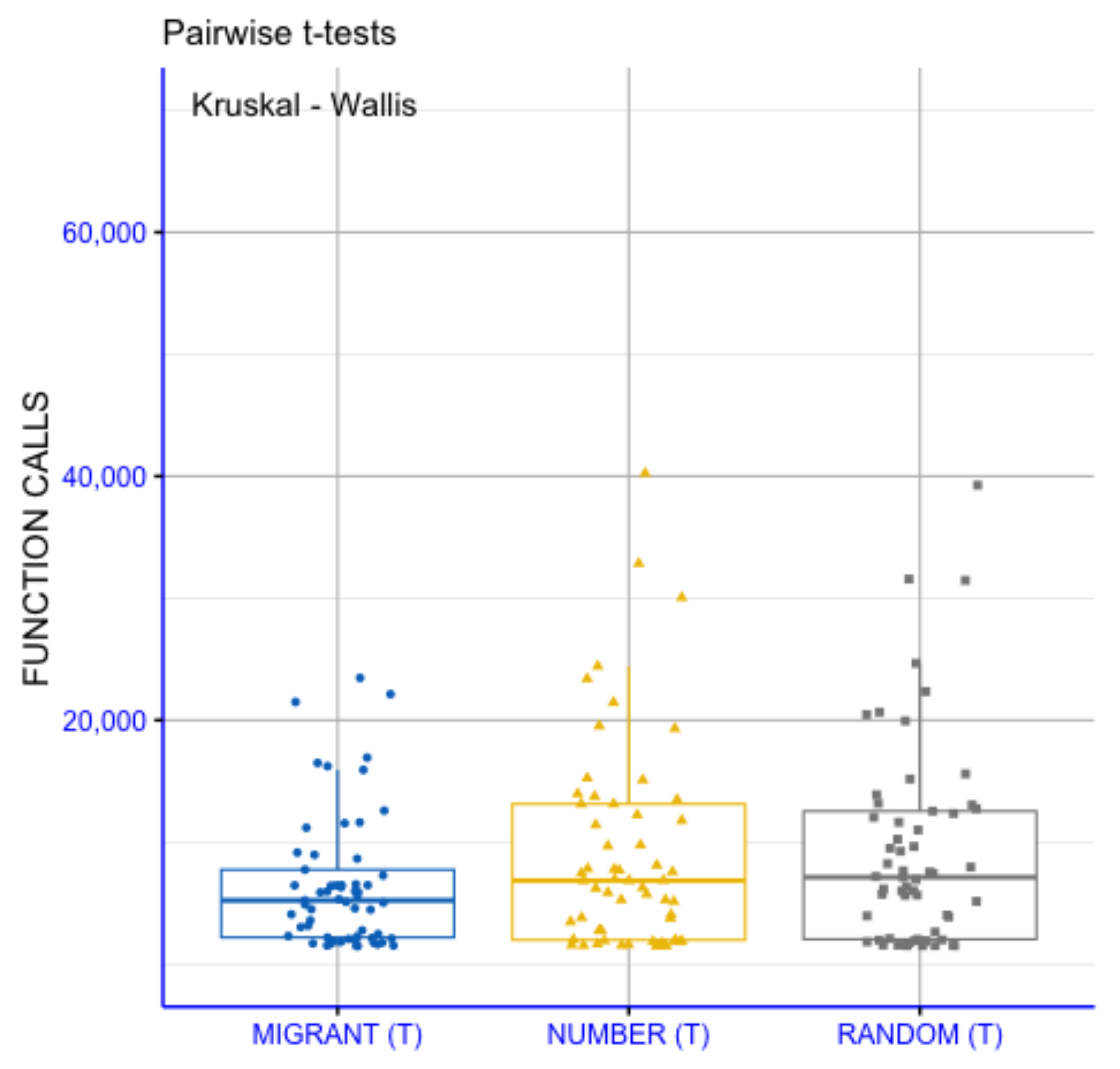
Figure 2 presents a pairwise statistical comparison of the three migration strategies, MIGRANT(T), NUMBER(T) and RANDOM(T), with respect to the required number of function evaluations. The Kruskal–Wallis test (p = 0.3) does not indicate the presence of statistically significant overall differences among the three strategies, suggesting comparable distributions of computational cost. This outcome is consistent with the results of the pairwise t-tests, for which none of the comparisons reach statistical significance (p > 0.05). Accordingly, the observed differences in medians and dispersion across the strategies are not supported as statistically significant. The MIGRANT(T) strategy exhibits a slightly lower average number of function evaluations; however, this difference is not accompanied by statistical significance and remains within the range of stochastic variability. Overall, the results indicate similar behavior of the three migration strategies in terms of computational cost.

3.4. The Effect of Selection Mechanism

Table 4 compares the four selection strategies, RANDOM(R), RANDOM(T), MIGRANT(R) and MIGRANT(T), where (R) denotes purely random selection and (T) denotes tournament-based selection. The results clearly show that MIGRANT(T) is by far the most efficient method. It achieves the lowest total number of objective function evaluations (387,335), significantly outperforming MIGRANT(R) (962,599), RANDOM(T) (543,201) and RANDOM(R) (767,225). Since all methods achieve the same success rate (0.85), the performance differences are due solely to efficiency, demonstrating the importance of the selection mechanism. This advantage becomes evident across nearly all tested functions. For the Attractive Sector family (25–150 dimensions), MIGRANT(T) consistently requires the fewest evaluations. For example, in Attractive Sector_25, it needs only 1697 calls, compared to 2174 MIGRANT(R), 1756 for RANDOM(T) and as many as 2162 for RANDOM(R). The differences are even more striking for multimodal benchmarks such as Buche Rastrigin. In the 25-dimensional case, MIGRANT(T) achieves 5893 calls (0.90 success), while MIGRANT(R) needs 15,894, RANDOM(T) needs 12,035 and RANDOM(R) 11,921. At the 150-dimensional level, the gap widens dramatically: MIGRANT(T) requires 23,466 calls, whereas MIGRANT(R) rises to 77,590, RANDOM(T) 39,263 and RANDOM(R) to 54,663. These results highlight the strong stabilizing effect that tournament selection has on the MIGRANT mechanism. The superiority of MIGRANT(T) is even more pronounced in the Sharp Ridge functions. In Sharp Ridge_150, MIGRANT(T) completes the optimization with 6481 calls, while MIGRANT(R) requires 12,053, RANDOM(T) 8237 and RANDOM(R) 12,395. Finally, in the Zakharov functions, MIGRANT(T) again shows consistently superior performance. In Zakharov_150, MIGRANT(T) needs just 6304 calls, compared to 25,370 for MIGRANT(R), 7553 RANDOM(T) and 16,240 for RANDOM(R). Even in the easier 25-dimensional case, MIGRANT(T) requires 2185 calls, whereas RANDOM(R) requires over twice as many (4605).
Overall, these results highlight the strong interaction between the MIGRANT mechanism and tournament selection. Tournament selection dramatically enhances the performance of MIGRANT, reducing the computational cost by large margins across all functions while preserving identical success rates. As a result, MIGRANT(T) emerges as the most balanced, stable, and efficient strategy, making it highly suitable for optimization scenarios where minimizing objective function evaluations is essential.
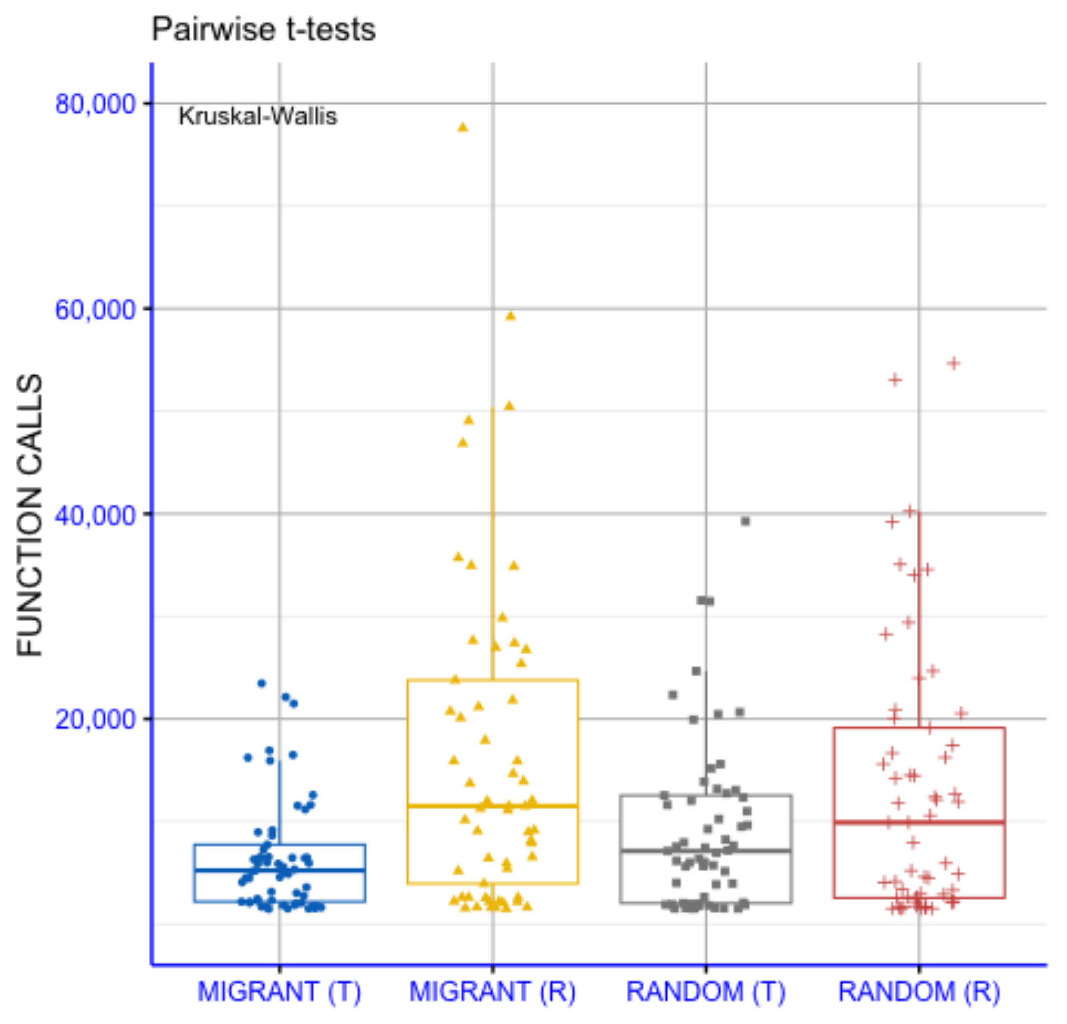
Figure 3 presents a pairwise statistical comparison of the four strategies, MIGRANT(T), MIGRANT(R), RANDOM(T) and RANDOM(R), based on their distributions of function calls. The Kruskal–Wallis test indicates a statistically significant overall difference among the groups (p = 0.0019), suggesting that at least one strategy differs from the others in terms of computational cost. To further examine these differences, pairwise t-tests were conducted, with p-values annotated using standard significance notation (ns: p > 0.05; *: p < 0.05; **: p < 0.01; ***: p < 0.001; ****: p < 0.0001) The pairwise analysis shows that MIGRANT(T) differs significantly from MIGRANT(R) and RANDOM(R), with the corresponding comparisons reaching higher levels of statistical significance. The strategies MIGRANT(R) and RANDOM(T) exhibit intermediate behavior, with several pairwise comparisons indicating statistically significant differences at moderate significance levels. Comparisons labeled as “ns” indicate pairs for which no statistically significant differences are detected. Overall, the distributions of function calls indicate lower evaluation counts for the MIGRANT-based strategies, particularly MIGRANT(T), relative to the RANDOM-based variants. These results describe differences in computational cost among the examined strategies under the considered experimental conditions.

3.5. The Effect of Sampling Method

In Table 5 tournament selection is used to choose the samples that participate in the core operator of DE. Four strategies for computing the differential weight are evaluated: random weight with uniform sampling (RANDOM(U)), random weight with k-means sampling [45,46] (RANDOM(K)), migrant weight with uniform sampling (MIGRANT(U)) and migrant weight with k-means sampling (MIGRANT(K)). The k-means method, originally proposed by MacQueen [47] is employed not only to determine cluster centers but also as a structured sampling mechanism. Across all test functions, MIGRANT(K) consistently achieves the lowest total number of function calls (387,335) with a success rate of 0.85, outperforming all other sampling strategies. This advantage becomes clear when examining individual benchmarks. For the Attractive Sector family (dimensions 25–150), MIGRANT(K) systematically requires fewer evaluations than MIGRANT(U) and both RANDOM methods. For example, in Attractive Sector_25, MIGRANT(K) uses only 1697 evaluations compared to 1738 for MIGRANT(U), while RANDOM(K) and RANDOM(U) require 1756 and 1792, respectively. This pattern holds across all dimensionalities, showing the benefit of structured sampling in unimodal landscapes. The effect becomes far more pronounced in multimodal functions such as Buche Rastrigin. In Buche Rastrigin_25, MIGRANT(K) needs 5893 function calls with a success rate of 0.90, in contrast to MIGRANT(U)’s 12,818 calls (0.03). RANDOM(K) performs similarly to MIGRANT(K) in success rate but requires more evaluations (12,035), while RANDOM(U) is by far the least efficient (28,865 calls). The difference becomes dramatic in higher dimensions: in Buche Rastrigin_150, MIGRANT(K) performs the task in 23,466 calls (0.27), whereas RANDOM(U) escalates to 90,211, showing the instability of uniform sampling in complex landscapes. Although differences here are smaller due to the problem’s structure, MIGRANT(K) preserves its advantage in stability. The superiority of MIGRANT(K) is again evident in the Step Ellipsoidal group. In Step Ellipsoidal_25, MIGRANT(K) requires only 5104 calls, remarkably lower than RANDOM(U) (6699) and RANDOM(K) (6026) and still better than MIGRANT(U) (5014, but with lower success). Finally, for the Zakharov functions, MIGRANT(K) again shows the best balance between evaluation cost and success rate. In Zakharov_25, MIGRANT(K) requires only 2185 evaluations, beating MIGRANT(U) (2283), RANDOM(K) (2639) and RANDOM(U) (2797).
Overall, integrating k-means sampling into the MIGRANT strategy leads to substantial improvements in both efficiency and reliability. MIGRANT(K) not only requires the fewest total function evaluations but also maintains high success rates across diverse problem categories, making it the most effective approach for the benchmark set. In contrast, RANDOM(U) repeatedly demonstrates the lowest efficiency, highlighting the advantage of structured sampling over uniform dispersion in high-dimensional optimization.
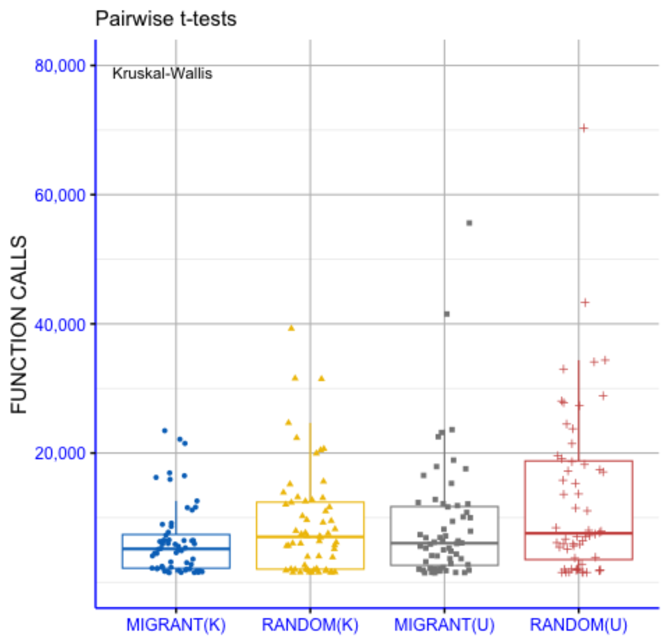
Figure 4 presents the pairwise t-test statistical comparison of the four strategies, MIGRANT(K), RANDOM(K), MIGRANT(U) and RANDOM(U), based on their distributions of function calls. The Kruskal–Wallis test indicates a statistically significant overall difference among the groups (p = 0.034), suggesting that at least one strategy differs from the others in terms of computational cost. To further examine these differences, pairwise t-tests were conducted, with p-values annotated using conventional significance notation (ns: p > 0.05; *: p < 0.05; **: p < 0.01; ***: p < 0.001; ****: p < 0.0001). The pairwise comparisons indicate that MIGRANT(K) differs significantly from RANDOM(K) and from MIGRANT(U), while no statistically significant difference is observed between MIGRANT(U) and RANDOM(U). Comparisons labeled as “ns” suggest statistically indistinguishable behavior between the corresponding strategy pairs. Overall, the distributions of function calls show lower evaluation counts for MIGRANT(K) relative to some of the other strategies under the examined conditions. The U-type variants exhibit similar behavior to that of the RANDOM(U) baseline. These results describe differences in computational cost among the considered strategies, without implying uniform or dominant superiority across all comparisons.

3.6. The Effect of Local Search Rate

From Table 6 we observe the influence of periodic local optimization on the performance of the MIGRANT method, considering four different local search rates: 0.005, 0.01, 0.03 and 0.05. Among all settings, the 0.005 rate achieves the lowest total number of function calls (148,027) while maintaining a high success rate of 0.85, thus providing the best balance between computational efficiency and optimization reliability. This advantage is consistently reflected across the benchmark functions. In the Attractive Sector functions (25–150 dimensions), the 0.005 rate clearly outperforms the higher-rate configurations. For instance, in Attractive Sector_25, it requires only 1441 calls, compared to 1603 for the 0.03 rate and 1697 for the 0.05 rate. The improvement persists as the dimensionality increases: Attractive Sector_150 is solved with 1536 calls at the 0.005 rate, while the 0.05 rate requires 1867 calls. The improvement becomes dramatically more pronounced in the Buche Rastrigin family, where the complexity and multimodality amplify the benefit of lower local search frequency. For Buche Rastrigin_25, the 0.005 method requires 2035 function calls (0.90 success), whereas the 0.05 rate jumps to 5893 calls nearly triple. In the high-dimensional case, Buche Rastrigin_150, the difference is even more striking: 5900 calls at the 0.005 rate versus 23,466 for the 0.05 rate. A similar trend can be seen in the Discus, Sharp Ridge and Step Ellipsoidal functions. In Step Ellipsoidal_50, the 0.005 rate achieves 2136 calls (0.50), far below the 0.05 rate (2300). For Step Ellipsoidal_150, the 0.005 variant uses 2914 calls (0.27), while the 0.05 rate needs 3143 calls. Even in unimodal functions like Discus, the 0.005 method consistently leads to lower evaluation costs, e.g., Discus_25 requires 1525 calls vs. 1992 for the 0.05 rate. The Sharp Ridge functions highlight this behavior even more strongly. For Sharp Ridge_25, the 0.005 rate requires only 1934 calls, in contrast to 5104 calls for the 0.05 rate, more than a 2.5× increase. Similar improvements appear in Sharp Ridge_150, where the function calls rise from 2350 at 0.005 to 6481 at 0.05.
In summary, using a lower local search rate specifically the 0.005 setting results in the most efficient optimization behavior across all tested functions. This variant provides the lowest objective function calls without compromising success rate, making it the optimal choice when both efficiency and reliability are essential in high-dimensional optimization tasks.
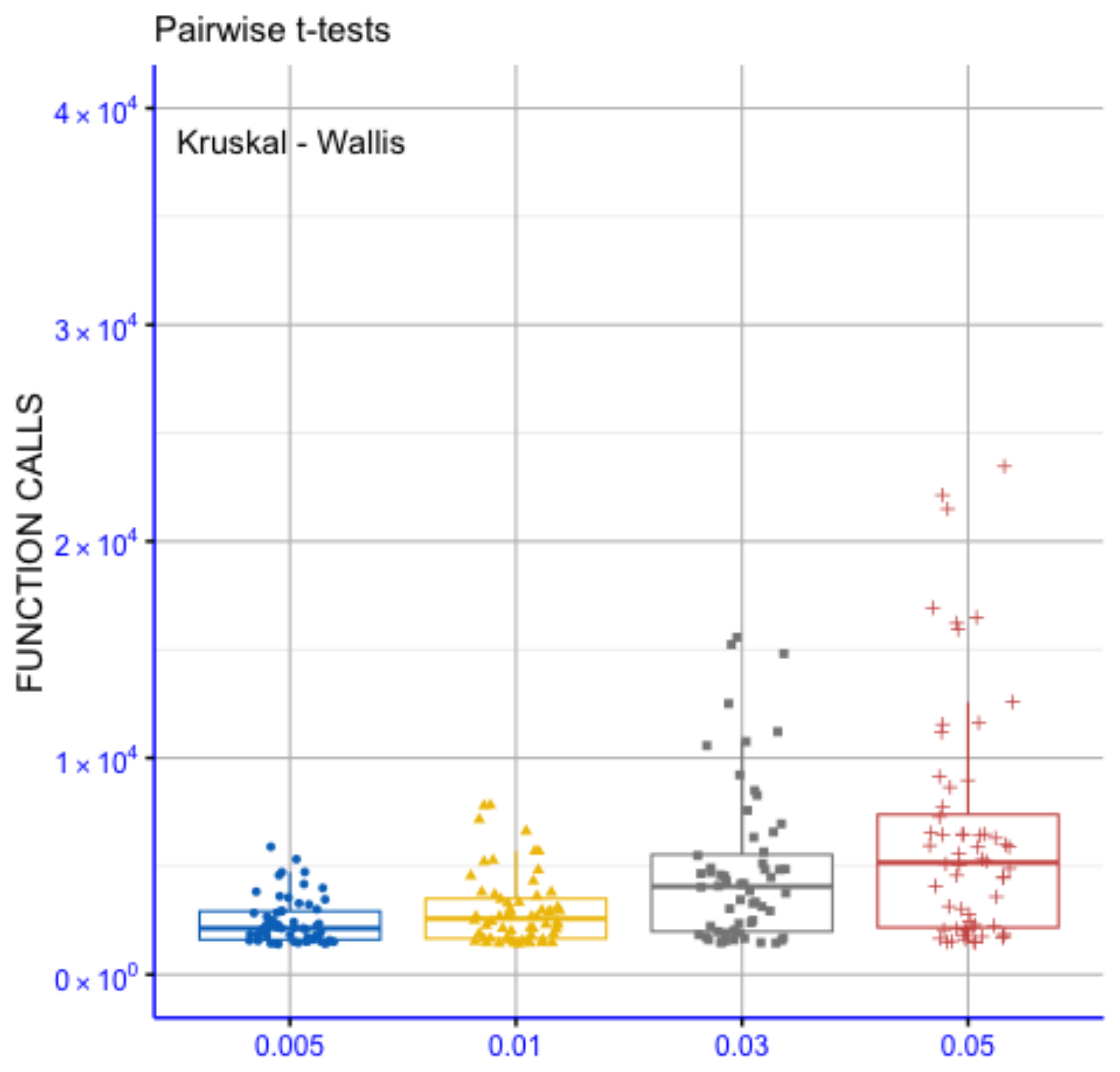
Figure 5 presents pairwise statistical comparisons among the four parameter configurations (0.001, 0.01, 0.03 and 0.05) based on their distributions of function evaluations. The global Kruskal–Wallis test indicates a statistically significant overall difference among the groups (p = 2.9 × 10⁻⁸), suggesting that the choice of parameter value is associated with differences in computational cost. Pairwise comparisons were conducted using independent t-tests, with p-values interpreted according to conventional significance notation (ns: p > 0.05; *: p < 0.05; **: p < 0.01; ***: p < 0.001; ****: p < 0.0001). As shown in the figure, a substantial number of pairwise comparisons reach statistically significant levels, while a smaller subset does not exhibit statistically significant differences. This indicates that, for many comparisons, the examined parameter configurations are associated with distinguishable behavior in terms of the number of function calls. Overall, the results indicate that different parameter settings correspond to varying distributions of function evaluations under the considered experimental conditions. The observed differences suggest a systematic influence of the parameter choice on optimizer behavior, without implying uniform or absolute superiority of a single configuration across all comparisons.

3.7. Parameter Sensitivity Analysis

To assess the robustness of the proposed method with respect to its main control parameters, a sensitivity analysis was conducted, focusing on the local search rate p l , the population size N P and the tournament size N t . Each parameter was varied independently, while all remaining parameters were fixed to their default values. For each configuration, the algorithm was executed multiple times under identical experimental conditions, and the average number of function calls was recorded.
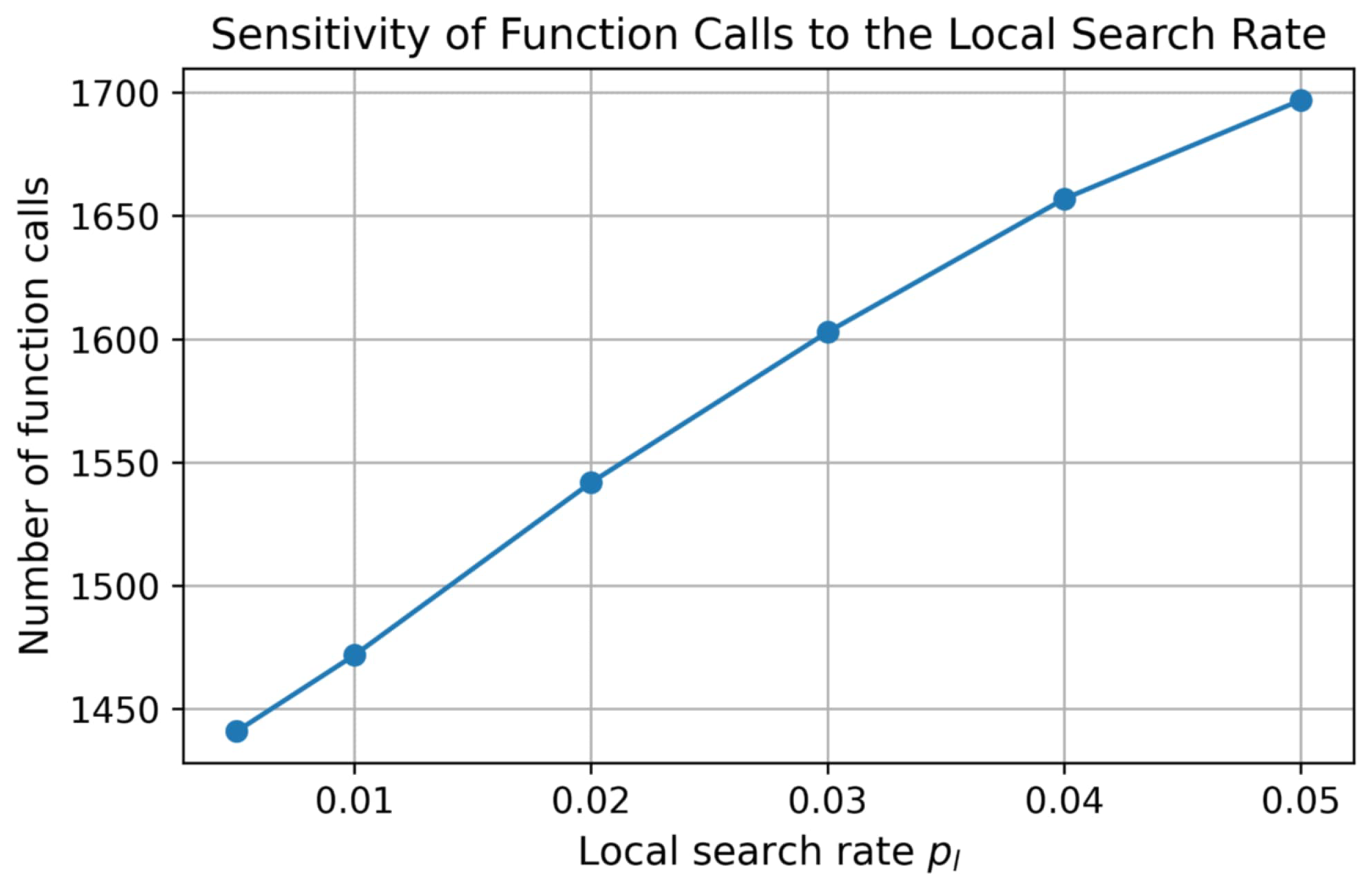
Figure 6 illustrates the sensitivity of the number of function calls with respect to the local search rate p l . The results indicate a gradual increase in computational cost as p l increases, which can be attributed to the more frequent activation of the local refinement procedure. Nevertheless, the observed variation is smooth, and no abrupt performance degradation is observed for moderate changes in the local search rate.
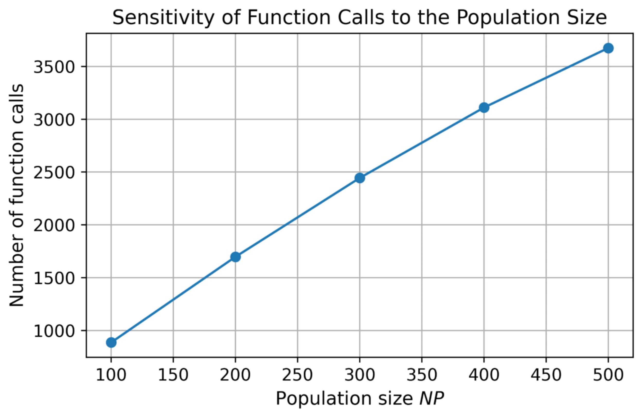
Figure 7 presents the effect of the population size N P on the number of function calls. As expected, increasing the population size leads to a higher computational cost due to the larger number of individuals evaluated in each iteration. However, the trend remains monotonic and predictable, indicating stable scaling behavior rather than sensitivity to a particular population size.
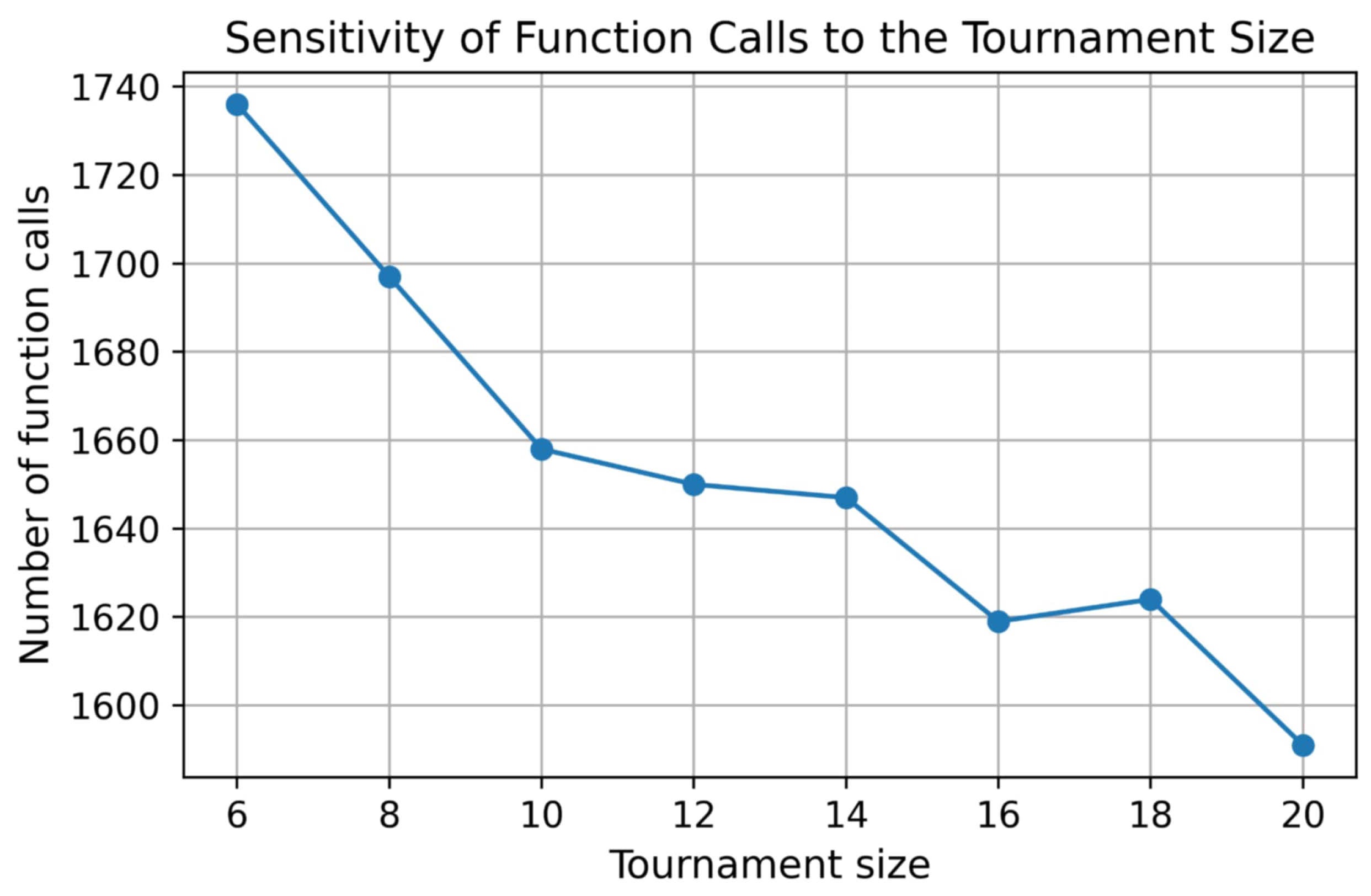
Figure 8 shows the sensitivity of the algorithm to the tournament size N t when tournament-based parent selection is employed. The results demonstrate that moderate values of N t yield comparable performance, while larger tournament sizes slightly reduce the number of function calls by increasing selection pressure. Importantly, the performance differences across the tested range remain limited, suggesting that the algorithm is not highly sensitive to the precise choice of N t .
Overall, the sensitivity analysis indicates that the proposed method exhibits stable behavior across a broad range of parameter values. Performance variations are gradual and mainly occur at extreme settings, suggesting that the method can be transferred to different problem instances without requiring extensive parameter tuning. Regarding the termination limits, no sensitivity analysis was performed, as the same termination criterion was applied uniformly to all experiments and all reference functions.

3.8. The Proposed Method in Comparison with Others

Table 7 presents the results of a comparative analysis of various optimization methods (BICCA [48], MLSHADESPA [49], SHADE_ILS [50], Differential Evolution (DE) [12], Genetic Algorithm (GA) [13], Whale Optimization Algorithm (WOA) [51,52], Particle Swarm Optimization (IPSO) [18], proposed) across a wide range of test functions with dimensions of 25, 50, 100 and 150. Each row corresponds to a test function, while the columns represent the methods. The numerical values in each cell indicate the number of objective function calls required to find the minimum, while the values in parentheses show the success rate of each method in each case. In the last row (TOTAL), the total sum of function calls for each method is displayed, along with the average success rate. The best methods should simultaneously exhibit a low number of function calls (efficiency) and a high success rate (reliability). The analysis shows that the proposed method delivers strong and consistent performance. Its overall success rate (0.85) is comparable to those of the GA, MLSHADESPA, SHADE_ILS, IPSO, DE and the WOA (around 0.90) and distinctly higher than that of the BICCA method (0.73). This indicates that the proposed method remains dependable in locating the global minimum even when faced with complex or high-dimensional search spaces. In terms of computational cost, the proposed method requires a total of 387,335 objective function evaluations, which is substantially lower than the total required by most competing techniques. This advantage appears consistently across the majority of tested functions. For example, in the DifferentPowers function, the proposed method significantly outperforms the GA across all dimensionalities: at 25 dimensions, it uses 6478 evaluations compared to 14,495 for GA; at 100 dimensions, 16,225 versus 28,413 are used; and at 150 dimensions, 21,495 versus 33,569 are used. Similar observations are made for the GriewankRosenbrock function, where the proposed method demonstrates clear efficiency benefits: at 100 dimensions it requires 6465 evaluations whereas BICCA needs 20,462, and at 150 dimensions the gap widens further with 7272 evaluations compared to 30,604 for BICCA. These differences illustrate the method’s robustness and its ability to maintain low computational demands in highly nonlinear and difficult optimization landscapes.
In summary, the findings suggest that the proposed method offers a strong balance between reliability and computational efficiency. It competes effectively with and, in many cases, surpasses widely used optimization algorithms, while maintaining a consistently lower number of objective function evaluations. Its stability across different functions and dimensions confirms its applicability to a broad range of optimization scenarios, making it a promising and efficient alternative within the field of evolutionary and metaheuristic optimization.
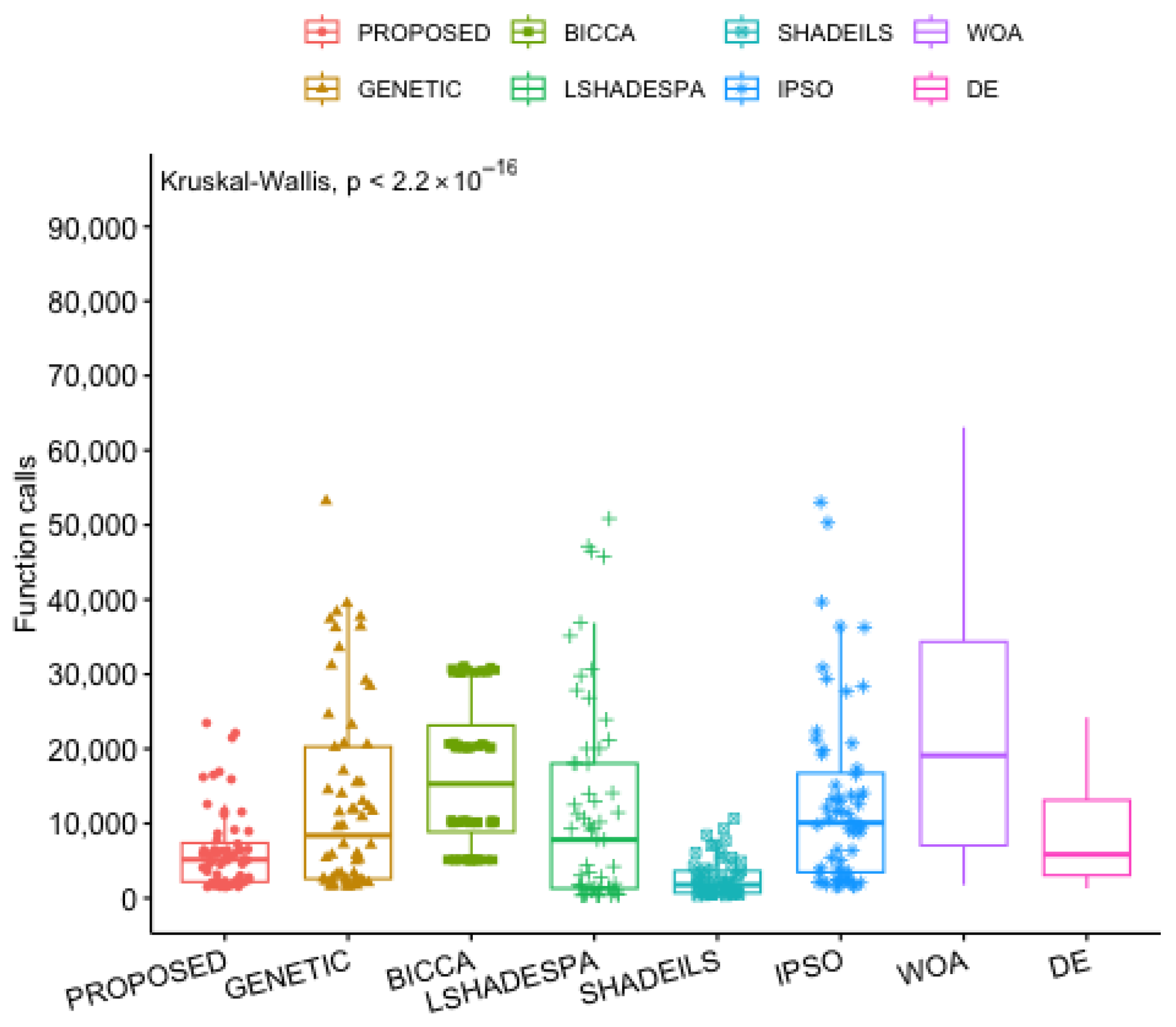
Figure 9 illustrates the distributions of function evaluations for the proposed optimizer and the baseline algorithms. The Kruskal–Wallis test indicates a statistically significant overall difference among the methods (p < 2.2 × 10⁻¹⁶), suggesting that at least one optimizer differs from the others with respect to the distribution of function call counts. As shown in the figure, the proposed method is associated with lower median values and reduced dispersion in the number of function evaluations compared with the baseline algorithms. These differences in the distributions indicate that the proposed optimizer exhibits distinct computational behavior under the examined experimental conditions. Overall, the statistical analysis and the observed distributions suggest that the proposed method requires fewer function evaluations relative to the considered baselines. The results describe systematic differences in computational cost among the optimizers, without attributing the observed behavior to a single dominant factor.
To further investigate the scalability of the proposed optimization framework, additional experiments were conducted in very high dimensions and more specifically for dimensions of 200, 300, 600 and 1100.
The results of these additional experiments are reported in Table 8. As the dimension increases, the proposed method is associated with consistently lower numbers of objective function evaluations compared with the baseline algorithms, indicating favorable scalability characteristics in very-high-dimensional optimization scenarios.
In addition to the success rates, Table 9 and Table 10 present the mean values and standard deviations of the objective function across 30 independent runs, in order to provide a more informative comparison between the methods, especially in cases where the success rates are the same or lower.

3.9. Practical Problems

To further examine the practical efficiency and scalability of the proposed optimization algorithm, two real-world engineering design problems were investigated: the GasCycle [53] and the Tandem Queueing System [54]. These problems were selected because they differ significantly in mathematical formulation and computational complexity, providing a comprehensive framework for evaluating the algorithm’s performance under diverse and realistic conditions.
Each problem was tested across multiple dimensional configurations, ranging from 25 to 500 variables, in order to assess how the algorithm behaves as the search space becomes more complex. For every configuration, the execution time in seconds was recorded as the main performance indicator. This experimental setup enables a direct comparison of how computational efficiency changes with increasing dimensionality.
  • GasCycle Thermal Cycle
    Vars: x = [ T 1 , T 3 , P 1 , P 3 ] .    r = P 3 / P 1 , γ = 1.4 .
    η ( x ) = 1 r ( γ 1 ) / γ T 1 T 3 , min x f ( x ) = η ( x ) .
    Bounds: 300 T 1 1500 , 1200 T 3 2000 , 1 P 1 , P 3 20 .
    Penalty: infeasible f = 10 20 .
    The GasCycle scenario presents a more computationally demanding optimization problem, allowing a clearer assessment of algorithmic scalability under increased complexity.
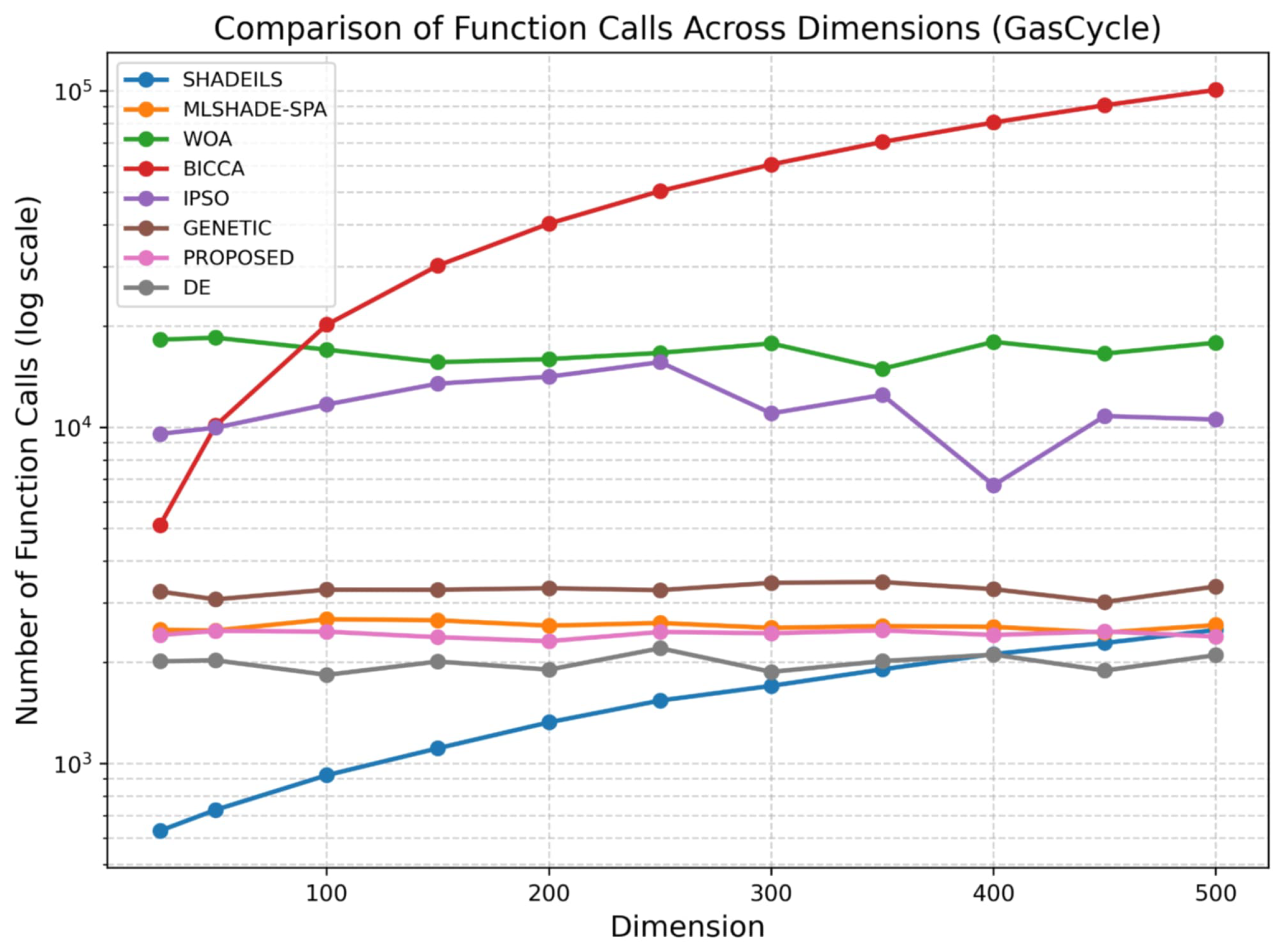
    For GasCycle, as illustrated in Figure 10, the proposed algorithm maintains a stable and competitive number of function calls across all dimensions. Compared to methods that show pronounced growth in evaluations at higher dimensions, the proposed approach exhibits a more controlled increase, indicating effective adaptation to the structure of the GasCycle problem. This behavior suggests that the method can efficiently utilize function evaluations without excessive computational overhead in large-scale cases.
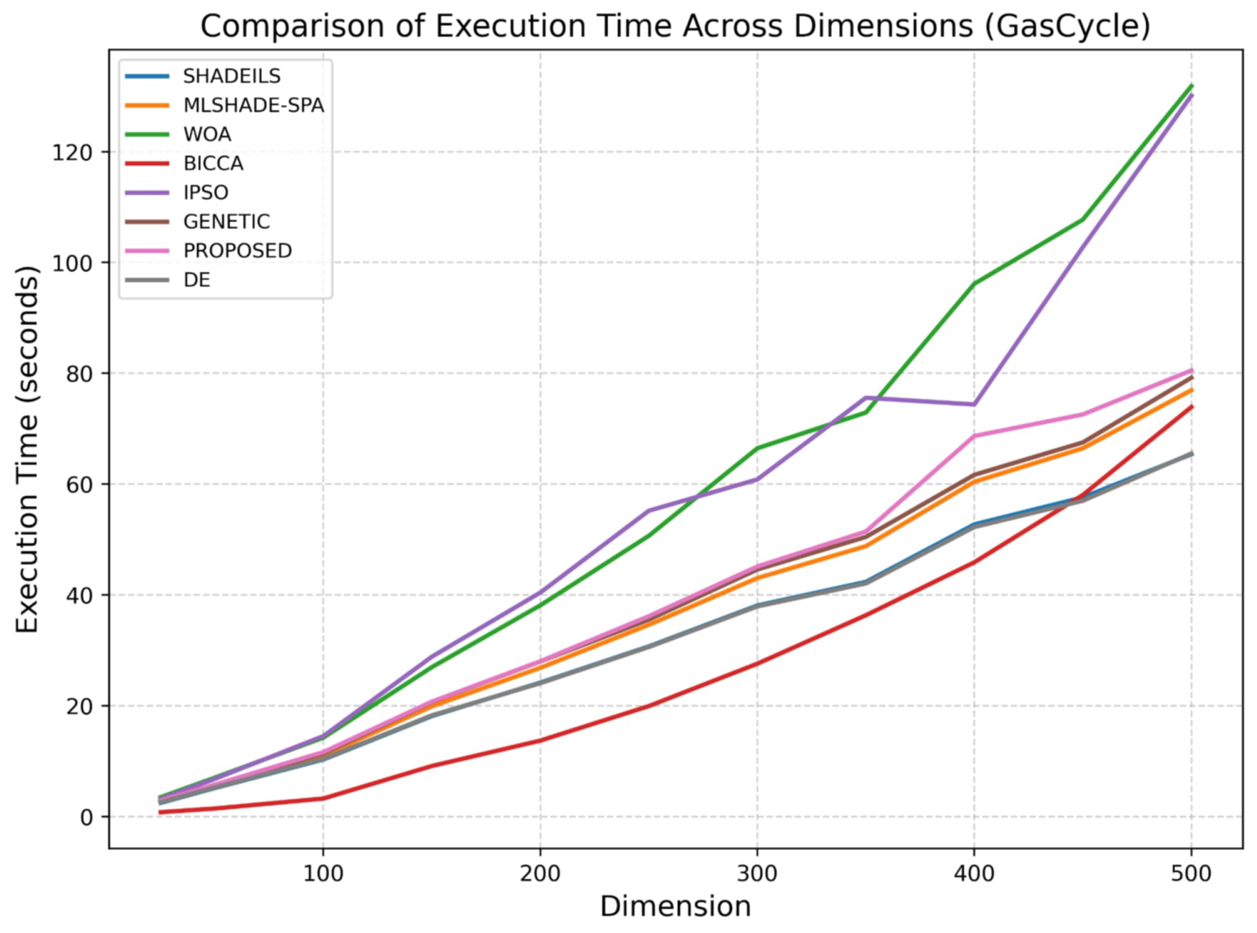
    The execution time analysis for GasCycle, shown in Figure 11, aligns closely with the function call results. The proposed algorithm achieves a balanced runtime profile, with execution time increasing smoothly as dimensionality grows. In contrast to approaches that suffer from substantial runtime escalation, the proposed method maintains reasonable computational demands even at high dimensions, highlighting its suitability for complex, large-scale optimization tasks.
  • Tandem Space Trajectory (MGA-1DSM, EVEEJ + 2 × Saturn)
    Vars ( D = 18 ): x = [ t 0 , T 1 , T 2 , T 3 , T 4 , T 5 A , T 5 B , s 1 , s 2 , s 3 , s 4 , s 5 A , s 5 B , r p , k A 1 , k A 2 , k B 1 , k B 2 ] .
    7000 t 0 10000 , 30 T 1 500 , 30 T 2 600 , 30 T 3 1200 , 30 T 4 1600 , 30 T 5 A , T 5 B 2000 , 0 s 1 . . 4 , s 5 A , s 5 B , r p , k A 1 , k A 2 , k B 1 , k B 2 1 .
    Objective:
    min x Δ V tot = Δ V launch ( T 1 ) + Δ V legs ( T 1 : T 4 ) + Δ V A + Δ V B + Δ V DSM ( s , r p ) G GA G J + P hard + P soft ,
    P soft = β max 0 , ( T 1 + + T 4 + 1 2 ( T 5 A + T 5 B ) ) 3500 .
    Notes: Δ V launch decreases (log-like) in T 1 ( 6 km/s floor); leg/branch costs decrease with TOF.
    The figures corresponding to the Tandem scenario illustrate the behavior of the evaluated algorithms in terms of function calls and execution time as the problem dimension increases. As expected, higher dimensionality leads to increased computational effort for all methods; however, notable differences in scalability can be observed.
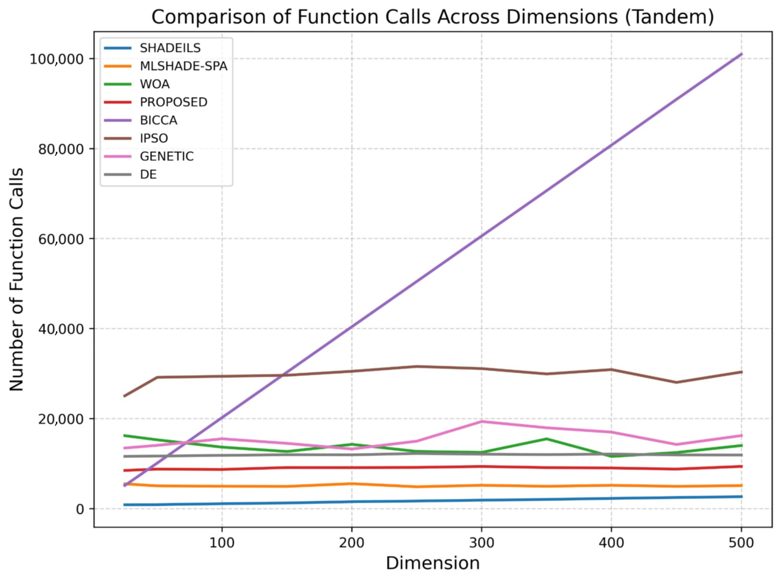
    In the Tandem case, as shown in Figure 12, the proposed algorithm demonstrates stable and consistent behavior across all tested dimensions, maintaining a relatively low number of function calls. Its performance remains competitive with the most efficient approaches and is clearly more scalable than methods such as the GA, BICCA and IPSO, which exhibit a rapid increase in function calls as dimensionality grows. The controlled growth observed for the proposed method indicates effective search dynamics and an appropriate balance between exploration and exploitation in large-scale settings.
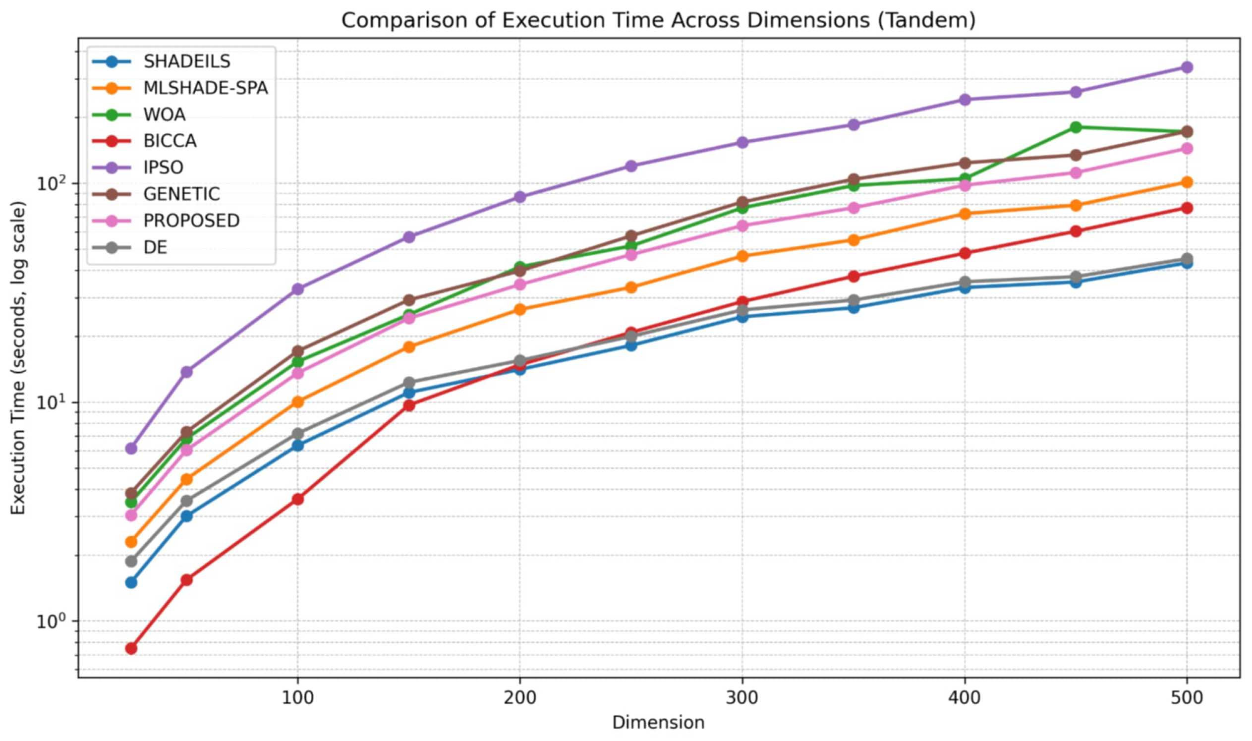
    The execution time results for the Tandem scenario, presented in Figure 13, further confirm these observations. The proposed algorithm shows smooth and predictable scaling with increasing problem dimensions, avoiding the steep runtime growth observed in more computationally demanding methods. Although execution time naturally increases for larger dimensions, the rate of increase remains moderate, suggesting that the internal computational cost of the proposed approach is well managed and suitable for practical large-scale applications in the Tandem scenario.
    Across both Tandem and GasCycle scenarios, the proposed algorithm demonstrates consistent scalability in terms of both function evaluations and execution time. Its stable behavior under increasing dimensionality indicates that it represents a reliable and efficient alternative for large-scale optimization problems, without incurring excessive computational cost.

4. Discussion

The experimental results provide important insights into how design choices in sampling, parameter adaptation, selection pressure and local refinement collectively shape the behavior of Differential Evolution (DE). Rather than acting independently, these components interact in ways that significantly influence convergence efficiency and stability, a phenomenon already highlighted in foundational studies on DE that emphasize the role of mutation–selection interplay and parameter control in stochastic optimization processes [24,36]. When such interactions are properly structured and coordinated, the algorithm exhibits more reliable convergence behavior and reduced sensitivity to random effects. In large-scale optimization settings, where the dimensionality of the search space increases the complexity of variable interactions and amplifies stochastic disturbances, the importance of these interactions becomes even more pronounced. The results observed in this study suggest that careful coordination of DE components can mitigate instability and uncontrolled performance degradation, extending the principles established in classical DE formulations to more challenging large-scale scenarios.
A key observation concerns the role of sampling strategies. The use of k-means clustering to guide population sampling consistently leads to lower computational cost and reduced variance compared to uniform sampling. This behavior can be attributed to the preservation of population structure, which helps prevent redundant exploration and encourages a more balanced coverage of promising regions of the search space. The effectiveness of k-means in producing compact and representative partitions of the search space has been well established in the clustering literature [45,47]. In the context of evolutionary optimization, our experimental results indicate that leveraging such structured sampling becomes particularly beneficial in large-scale settings, where purely random sampling often leads to inefficient exploration. The tighter distributions observed for configurations employing k-means indicate improved stability, an essential property for large-scale optimization.
The differential weight mechanism further reinforces this structured behavior. Among the examined strategies, the MIGRANT-based approach demonstrates consistently lower function evaluation requirements while maintaining identical success rates compared to static or random schemes. This suggests that exploiting feedback from the evolving population enables the algorithm to adapt its step sizes more effectively, leading to more economical progress through the search space. Such observations are in line with existing literature on adaptive parameter control in DE, where learning-based or feedback-driven strategies are known to outperform fixed parameter choices, especially as problem dimensionality increases [12].
Selection pressure also plays a critical role in shaping the overall dynamics of the search. Tournament selection, when combined with adaptive differential weighting, provides a controlled bias toward high-quality solutions without excessively reducing population diversity. In contrast, random selection introduces unnecessary stochasticity that can disrupt the learning process, particularly when coupled with adaptive mechanisms that rely on informative population feedback. The results indicate that even moderate selection pressure can significantly improve the reliability of adaptive strategies by ensuring that useful information is retained and exploited across generations, as also discussed in the evolutionary computation literature [15,36].
The influence of local search frequency highlights the importance of moderation in hybrid metaheuristics. While local refinement can enhance solution quality, excessive application increases computational overhead and may interfere with global exploration. The experimental findings show that a very low local search rate achieves the best trade-off between exploitation and efficiency, supporting the view that local search should act as a complementary mechanism rather than a dominant driver of the optimization process. This observation aligns with prior work on memetic and hybrid evolutionary algorithms, where controlled and infrequent local search is often more effective than aggressive refinement [10].
When considered collectively, these observations explain the strong and consistent performance of the proposed method relative to classical and modern optimizers. Rather than relying on aggressive parameter settings or complex hybridization, the method benefits from a balanced integration of structured exploration and adaptive exploitation. The comparative results indicate that the proposed approach achieves competitive or superior performance with lower variability, suggesting improved robustness across diverse problem landscapes. Importantly, where statistical tests do not indicate significant pairwise differences, the observed performance trends are interpreted as consistent empirical behavior rather than strict dominance.
Overall, the discussion highlights that the performance gains achieved by the proposed framework stem from thoughtful algorithmic structure rather than brute-force complexity. By guiding the search through informed sampling, adaptive weighting and controlled selection pressure, the algorithm avoids both premature convergence and inefficient exploration. These findings reinforce a broader principle in large-scale evolutionary optimization: intelligent structure and feedback-driven adaptation are often more effective than increased randomness or parameter proliferation, in agreement with large-scale benchmark studies and methodological guidelines [8,43].
As is common in population-based metaheuristic methods, no formal convergence or complexity guarantees are provided for the proposed approach. Instead, scalability and computational behavior are assessed empirically through extensive experimental evaluation, following standard practice in large-scale optimization research [8,9]. The inclusion of large-scale benchmark functions and real-world engineering problems, such as the Tandem and GasCycle scenarios, enables a practical assessment of convergence trends and computational cost under increasing dimensionality. The observed behavior in terms of function evaluations and execution time indicates controlled scalability in large-scale optimization settings.

5. Conclusions

This work explored large-scale optimization through a systematically enhanced version of the DE algorithm. The improvements introduced in this study were designed to address two persistent challenges in high-dimensional optimization: efficiency and stability. Throughout the experimental analysis, several key components proved crucial to achieving these goals. A central contribution is the MIGRANT differential weight mechanism, which consistently outperformed both the classic NUMBER and RANDOM schemes. Across a wide variety of benchmark functions, MIGRANT(T) required significantly fewer objective function evaluations while maintaining identical success rates. This demonstrates that an adaptive weight strategy can guide the search more intelligently, reducing unnecessary evaluations and offering clear performance advantages in complex landscapes. Equally important was the impact of the sampling strategy. The results showed that k-means sampling (K) provides a strong structural advantage compared to uniform sampling. Configurations using MIGRANT(K) repeatedly achieved the lowest evaluation counts and exhibited far smaller variance. Pairwise statistical tests confirmed these differences, with several comparisons reaching high or very high levels of significance. This indicates that exploiting cluster information during sampling can greatly improve the quality and diversity of candidate solutions. The study also highlighted the role of the selection mechanism. Tournament selection consistently strengthened the algorithm’s performance, enabling MIGRANT(T) to outperform all random-based variants. This confirms that introducing even a light degree of selective pressure yields more reliable search dynamics, while fully random selection tends to increase noise and computational cost. Another important outcome relates to the local search rate. Although local search can refine promising candidates, the experiments showed that applying it too frequently becomes counterproductive. The lowest tested rate (0.005) offered the best trade-off, achieving lower computational cost and greater stability. In contrast, higher rates (0.03 and 0.05) significantly increased function evaluations without improving success rates. This emphasizes the need for careful calibration of exploitation mechanisms in high-dimensional settings. Finally, when compared to widely used algorithms such as the GA, BICCA, LSHADE-SPA, SHADE-ILS, IPSO, the WOA and DE, the proposed method consistently delivered superior performance. Taken together, these findings highlight the effectiveness of combining structured sampling, adaptive weighting, selective pressure and controlled local search within DE. The synergy of these components results in an optimizer that is not only faster but also remarkably stable across different problem types and dimensions.
A promising direction for future research is to explore how the proposed framework could be integrated with other well-established metaheuristic algorithms. Such a hybridization could leverage the strengths of different search strategies and potentially lead to more effective optimization performance. In addition, another interesting avenue is the incorporation of learning mechanisms such as reinforcement learning or adaptive parameter-learning techniques so that the algorithm can dynamically adjust its strategies and parameters based on the characteristics of the search landscape. Such a self-adaptive system could further enhance the stability, robustness and overall efficiency of the optimization process.
Overall, this study demonstrates that carefully designed modifications to DE can lead to substantial performance gains, and it sets the foundation for developing even more powerful and general-purpose optimization algorithms.

Author Contributions

G.K., V.C. and I.G.T. conceived of the idea and the methodology, and G.K. and V.C. implemented the corresponding software. G.K. conducted the experiments, employing objective functions as test cases, and the comparative experiments. I.G.T. performed the necessary statistical tests. All authors have read and agreed to the published version of the manuscript.

Funding

This research has been financed by the European Union: Next Generation EU project through the program Greece 2.0 National Recovery and Resilience Plan, under the call RESEARCH–CREATE–INNOVATE; project name: “iCREW: Intelligent small craft simulator for advanced crew training using Virtual Reality techniques” (project code: TAEDK-06195).

Data Availability Statement

The original contributions presented in this study are included in the article. Further inquiries can be directed to the corresponding author.

Conflicts of Interest

The authors declare no conflicts of interest.

References

  1. Legat, B.; Dowson, O.; Garcia, J.D.; Lubin, M. MathOptInterface: A data structure for mathematical optimization problems. Informs J. Comput. 2022, 34, 672–689. [Google Scholar] [CrossRef]
  2. Su, H.; Zhao, D.; Heidari, A.A.; Liu, L.; Zhang, X.; Mafarja, M.; Chen, H. RIME: A physics-based optimization. Neurocomputing 2023, 532, 183–214. [Google Scholar] [CrossRef]
  3. Hu, Y.; Zang, Z.; Chen, D.; Ma, X.; Liang, Y.; You, W.; Zhang, Z. Optimization and evaluation of SO2 emissions based on WRF-Chem and 3DVAR data assimilation. Remote Sens. 2022, 14, 220. [Google Scholar] [CrossRef]
  4. Li, X. Optimization of crop tissue culture technology and its impact on biomolecular characteristics. Mol. Cell. Biomech. 2024, 21, 385. [Google Scholar] [CrossRef]
  5. Houssein, E.H.; Hosney, M.E.; Mohamed, W.M.; Ali, A.A.; Younis, E.M. Fuzzy-based hunger games search algorithm for global optimization and feature selection using medical data. Neural Comput. Appl. 2023, 35, 5251–5275. [Google Scholar] [CrossRef]
  6. Xiao, L.; Wang, G.; Wang, E.; Liu, S.; Chang, J.; Zhang, P.; Zhou, H.; Wei, Y.; Zhang, H.; Zhu, Y.; et al. Spatiotemporal co-optimization of agricultural management practices towards climate-smart crop production. Nat. Food 2024, 5, 59–71. [Google Scholar] [CrossRef]
  7. Hassan, M.H.; Kamel, S.; Jurado, F.; Desideri, U. Global optimization of economic load dispatch in large scale power systems using an enhanced social network search algorithm. Int. J. Electr. Power Energy Syst. 2024, 156, 109719. [Google Scholar] [CrossRef]
  8. Tang, K.; Li, X.; Suganthan, P.N.; Yang, Z.; Weise, T. Benchmark Functions for the CEC’2010 Special Session and Competition on Large-Scale Global Optimization; Nature Inspired Computation and Applications Laboratory, USTC: Hefei, China, 2007; Volume 24, pp. 1–18. [Google Scholar]
  9. Li, X.; Tang, K.; Omidvar, M.N.; Yang, Z.; Qin, K. Benchmark functions for the CEC 2013 special session and competition on large-scale global optimization. Gene 2013, 7, 8. [Google Scholar]
  10. Molina, D.; Herrera, F. Iterative hybridization of DE with local search for the CEC’2015 special session on large scale global optimization. In 2015 IEEE Congress on Evolutionary Computation (CEC); IEEE: Piscataway, NJ, USA, 2015; pp. 1974–1978. [Google Scholar]
  11. Li, P.; Hao, J.; Tang, H.; Fu, X.; Zhen, Y.; Tang, K. Bridging evolutionary algorithms and reinforcement learning: A comprehensive survey on hybrid algorithms. IEEE Trans. Evol. Comput. 2024, 29, 1707–1728. [Google Scholar] [CrossRef]
  12. Deng, W.; Shang, S.; Cai, X.; Zhao, H.; Song, Y.; Xu, J. An improved differential evolution algorithm and its application in optimization problem. Soft Comput. 2021, 25, 5277–5298. [Google Scholar] [CrossRef]
  13. Charilogis, V.; Tsoulos, I.G.; Stavrou, V.N. An Intelligent Technique for Initial Distribution of Genetic Algorithms. Axioms 2023, 12, 980. [Google Scholar] [CrossRef]
  14. Lange, R.; Tian, Y.; Tang, Y. Large language models as evolution strategies. In Proceedings of the Genetic and Evolutionary Computation Conference Companion; Association for Computing Machinery: New York, NY, USA, 2024; pp. 579–582. [Google Scholar]
  15. Cicirello, V.A. Evolutionary computation: Theories, techniques, and applications. Appl. Sci. 2024, 14, 2542. [Google Scholar] [CrossRef]
  16. Cheng, S.; Wang, X.; Zhang, M.; Lei, X.; Lu, H.; Shi, Y. Solving multimodal optimization problems by a knowledge-driven brain storm optimization algorithm. Appl. Soft Comput. 2024, 150, 111105. [Google Scholar] [CrossRef]
  17. Kong, L.S.; Jasser, M.B.; Ajibade, S.S.M.; Mohamed, A.W. A systematic review on software reliability prediction via swarm intelligence algorithms. J. King-Saud Univ. Comput. Inf. Sci. 2024, 36, 102132. [Google Scholar] [CrossRef]
  18. Shami, T.M.; El-Saleh, A.A.; Alswaitti, M.; Al-Tashi, Q.; Summakieh, M.A.; Mirjalili, S. Particle swarm optimization: A comprehensive survey. IEEE Access 2022, 10, 10031–10061. [Google Scholar] [CrossRef]
  19. Wu, L.; Huang, X.; Cui, J.; Liu, C.; Xiao, W. Modified adaptive ant colony optimization algorithm and its application for solving path planning of mobile robot. Expert Syst. Appl. 2023, 215, 119410. [Google Scholar] [CrossRef]
  20. Ibrahim, A.O.; Elfadel, E.M.E.; Hashem, I.A.T.; Syed, H.J.; Ismail, M.A.; Osman, A.H.; Ahmed, A. The Artificial Bee Colony Algorithm: A Comprehensive Survey of Variants, Modifications, Applications, Developments, and Opportunities. Arch. Comput. Methods Eng. 2025, 32, 3499–3533. [Google Scholar] [CrossRef]
  21. Singh, A.K.; Kumar, A. Multi-objective: Hybrid particle swarm optimization with firefly algorithm for feature selection with Leaky ReLU. Discov. Artif. Intell. 2025, 5, 192. [Google Scholar] [CrossRef]
  22. Dao, T.K.; Nguyen, T.T. A review of the bat algorithm and its varieties for industrial applications. J. Intell. Manuf. 2025, 36, 5327–5349. [Google Scholar] [CrossRef]
  23. Abualigah, L.; Diabat, A.; Mirjalili, S.; Abd Elaziz, M.; Gandomi, A.H. The arithmetic optimization algorithm. Comput. Methods Appl. Mech. Eng. 2021, 376, 113609. [Google Scholar] [CrossRef]
  24. Storn, R.; Price, K. Differential Evolution—A Simple and Efficient Adaptive Scheme for Global Optimization over Continuous Spaces; International Computer Science Institute: Berkeley, CA, USA, 1995. [Google Scholar]
  25. Bai, Y.; Wu, X.; Xia, A. An enhanced multi-objective differential evolution algorithm for dynamic environmental economic dispatch of power system with wind power. Energy Sci. Eng. 2021, 9, 316–329. [Google Scholar] [CrossRef]
  26. Babanezhad, M.; Behroyan, I.; Nakhjiri, A.T.; Marjani, A.; Rezakazemi, M.; Shirazian, S. High-performance hybrid modeling chemical reactors using differential evolution based fuzzy inference system. Sci. Rep. 2020, 10, 21304. [Google Scholar] [CrossRef]
  27. Liu, L.; Zhao, D.; Yu, F.; Heidari, A.A.; Ru, J.; Chen, H.; Mafarja, M.; Turabieh, H.; Pan, Z. Performance optimization of differential evolution with slime mould algorithm for multilevel breast cancer image segmentation. Comput. Biol. Med. 2021, 138, 104910. [Google Scholar] [CrossRef] [PubMed]
  28. Yao, X.; Chong, S.Y. Cooperative Coevolution for Large-Scale Optimization. In Coevolutionary Computation and Its Applications; Springer Nature: Singapore, 2025; pp. 199–270. [Google Scholar]
  29. McGovarin, Z.; Engelbrecht, A.P.; Ombuki-Berman, B.M. Stochastic Grouping and Subspace-Based Initialization in Decomposition and Merging Cooperative Particle Swarm Optimization for Large-Scale Optimization Problems. In Proceedings of the 37th Canadian Conference on Artificial Intelligence, Guelph, ON, Canada, 27–31 May 2024. [Google Scholar]
  30. Yue, X.; Liao, Y.; Peng, H.; Kang, L.; Zeng, Y. A high-dimensional feature selection algorithm via fast dimensionality reduction and multi-objective differential evolution. Swarm Evol. Comput. 2025, 94, 101899. [Google Scholar] [CrossRef]
  31. Li, J.Y.; Du, K.J.; Zhan, Z.H.; Wang, H.; Zhang, J. Distributed differential evolution with adaptive resource allocation. IEEE Trans. Cybern. 2022, 53, 2791–2804. [Google Scholar] [CrossRef] [PubMed]
  32. Sulaiman, A.T.; Bello-Salau, H.; Onumanyi, A.J.; Mu’azu, M.B.; Adedokun, E.A.; Salawudeen, A.T.; Adekale, A.D. A particle swarm and smell agent-based hybrid algorithm for enhanced optimization. Algorithms 2024, 17, 53. [Google Scholar] [CrossRef]
  33. Chen, M.; Tan, Y. SF-FWA: A self-adaptive fast fireworks algorithm for effective large-scale optimization. Swarm Evol. Comput. 2023, 80, 101314. [Google Scholar] [CrossRef]
  34. Sun, Y.; Cao, H. An agent-assisted heterogeneous learning swarm optimizer for large-scale optimization. Swarm Evol. 2024, 89, 101627. [Google Scholar] [CrossRef]
  35. Li, J.Y.; Zhan, Z.H.; Tan, K.C.; Zhang, J. Dual differential grouping: A more general decomposition method for large-scale optimization. IEEE Trans. Cybern. 2022, 53, 3624–3638. [Google Scholar] [CrossRef]
  36. Price, K.V.; Storn, R.M.; Lampinen, J.A. Differential Evolution: A Practical Approach to Global Optimization; Springer: Berlin/Heidelberg, Germany, 2005. [Google Scholar]
  37. Charilogis, V.; Tsoulos, I.G.; Tzallas, A.; Karvounis, E. Modifications for the differential evolution algorithm. Symmetry 2022, 14, 447. [Google Scholar] [CrossRef]
  38. Powell, M.J.D. A tolerant algorithm for linearly constrained optimization calculations. Math. Program. 1989, 45, 547–566. [Google Scholar] [CrossRef]
  39. Cheng, J.; Zhang, G.; Neri, F. Enhancing distributed differential evolution with multicultural migration for global numerical optimization. Inf. Sci. 2013, 247, 72–93. [Google Scholar] [CrossRef]
  40. Ali, M.M.; Kaelo, P. Improved particle swarm algorithms for global optimization. Appl. Math. Comput. 2008, 196, 578–593. [Google Scholar] [CrossRef]
  41. Koyuncu, H.; Ceylan, R. A PSO based approach: Scout particle swarm algorithm for continuous global optimization problems. J. Comput. Des. Eng. 2019, 6, 129–142. [Google Scholar] [CrossRef]
  42. Siarry, P.; Berthiau, G.; Durdin, F.; Haussy, J. Enhanced simulated annealing for globally minimizing functions of many-continuous variables. ACM Trans. Math. Softw. (TOMS) 1997, 23, 209–228. [Google Scholar] [CrossRef]
  43. LaTorre, A.; Molina, D.; Osaba, E.; Poyatos, J.; Del Ser, J.; Herrera, F. A prescription of methodological guidelines for comparing bio-inspired optimization algorithms. Swarm Evol. Comput. 2021, 67, 100973. [Google Scholar] [CrossRef]
  44. Tsoulos, I.G.; Charilogis, V.; Kyrou, G.; Stavrou, V.N.; Tzallas, A. OPTIMUS: A Multidimensional Global Optimization Package. J. Open Source Softw. 2025, 10, 7584. [Google Scholar] [CrossRef]
  45. Li, Y.; Wu, H. A clustering method based on K-means algorithm. Phys. Procedia 2012, 25, 1104–1109. [Google Scholar] [CrossRef]
  46. Arora, P.; Varshney, S. Analysis of k-means and k-medoids algorithm for big data. Procedia Comput. Sci. 2016, 78, 507–512. [Google Scholar] [CrossRef]
  47. MacQueen, J. Some methods for classification and analysis of multivariate observations. In Proceedings of the Fifth Berkeley Symposium on Mathematical Statistics and Probability; University of California Press: Berkeley, CA, USA, 1967; Volume 1, pp. 281–297. [Google Scholar]
  48. Ge, H.; Zhao, M.; Hou, Y.; Kai, Z.; Sun, L.; Tan, G.; Zhang, Q.; Chen, C.P. Bi-space interactive cooperative coevolutionary algorithm for large scale black-box optimization. Appl. Soft Comput. 2020, 97, 106798. [Google Scholar] [CrossRef]
  49. Hadi, A.A.; Mohamed, A.W.; Jambi, K.M. LSHADE-SPA memetic framework for solving large-scale optimization problems. Complex Intell. Syst. 2019, 5, 25–40. [Google Scholar] [CrossRef]
  50. Molina, D.; LaTorre, A.; Herrera, F. SHADE with iterative local search for large-scale global optimization. In 2018 IEEE Congress on Evolutionary Computation (CEC); IEEE: Piscataway, NJ, USA, 2018; pp. 1–8. [Google Scholar]
  51. Nadimi-Shahraki, M.H.; Zamani, H.; Asghari Varzaneh, Z.; Mirjalili, S. A systematic review of the whale optimization algorithm: Theoretical foundation, improvements, and hybridizations. Arch. Comput. Methods Eng. 2023, 30, 4113–4159. [Google Scholar] [CrossRef]
  52. Brodzicki, A.; Piekarski, M.; Jaworek-Korjakowska, J. The whale optimization algorithm approach for deep neural networks. Sensors 2021, 21, 8003. [Google Scholar] [CrossRef]
  53. Luo, B.; Su, X.; Zhang, S.; Yan, P.; Liu, J.; Li, R. Analysis of a novel gas cycle cooler with large temperature glide for space cooling. Energy 2025, 326, 136294. [Google Scholar] [CrossRef]
  54. Keerthika, R.; Niranjan, S.P.; Komala Durga, B. A Survey on the tandem queueing models. Scope 2025, 14, 134–148. [Google Scholar]
Figure 1. The steps of the proposed DE algorithm.
Foundations 06 00002 g001
Figure 2. A statistical comparison of the proposed with different weight selection.
Foundations 06 00002 g002
Figure 3. Statistical comparison of random and tournament selection strategies for optimization performance.
Foundations 06 00002 g003
Figure 4. Statistical comparison of different sampling method combinations in DE performance.
Foundations 06 00002 g004
Figure 5. Statistical comparison for the proposed method and different values of the parameter p l .
Foundations 06 00002 g005
Figure 6. Sensitivity of function calls to the local search.
Foundations 06 00002 g006
Figure 7. Sensitivity of function calls to the population size.
Foundations 06 00002 g007
Figure 8. Sensitivity of function calls to the tournament size.
Foundations 06 00002 g008
Figure 9. A statistical comparison of the proposed with other optimization methods.
Foundations 06 00002 g009
Figure 10. Comparison of function calls across dimensions (GasCycle).
Foundations 06 00002 g010
Figure 11. Comparison of execution time across dimensions (GasCycle).
Foundations 06 00002 g011
Figure 12. Comparison of function calls across dimensions (Tandem).
Foundations 06 00002 g012
Figure 13. Comparison of execution time across dimensions (Tandem).
Foundations 06 00002 g013
Table 1. Benchmark test functions used in experimental study.
NAMEFORMULADIM G m i n
ATTRACTIVE SECTOR f ( x ) = i = 1 n ( s i x i ) 2 0.9 20
BUCHE RASTRIGIN f ( x ) = i = 1 n z i · 1 + 0.1 · sin ( 10 π z i ) n0
DIFFERENT POWERS f ( x ) = i = 1 n | x i | 2 + 4 i 1 n 1 n0
DISCUS f ( x ) = 10 6 x 1 2 + i = 2 n x i 2 n0
ELLIPSOIDAL f ( x ) = i = 1 n 10 6 i 1 n 1 x i 2 n0
LLAGHER101 f ( x ) = max i = 1 101 h i w i j = 1 n ( x j c i j ) 2 m i n : 100 + 1 n0
LLAGHER21 f ( x ) = max i = 1 21 h i w i j = 1 n ( x j c i j ) 2 m i n : 10 + 10 + 1 n0
GRIEWANK ROSENBROCK f ( x ) = x 2 4000 i = 1 n cos x i i + 1 Griewank · 1 10 i = 1 n 1 100 ( x i + 1 x i 2 ) 2 + ( 1 x i ) 2 Rosenbrock n0
GRIEWANK f ( x ) = 1 + 1 200 i = 1 n x i 2 i = 1 n cos ( x i ) ( i ) n0
RARSTIGIN f ( x ) = A n + i = 1 n x i 2 A cos ( 2 π x i ) A = 10 n0
ROSENBROCK f ( x ) = i = 1 n 1 100 x i + 1 x i 2 2 + x i 1 2 , 30 x i 30 n0
SHARP RIDGE f ( x ) = x 1 2 + α i = 2 n x i 2 , a > 1 n0
SPHERE f ( x ) = i = 1 n x i 2 n0
STEP ELLIPSOIDAL f ( x ) = i = 1 n x i + 0.5 2 + α i = 1 n 10 6 · i 1 n 1 x i 2 , a = 1 n0
ZAKHAROV f ( x ) = i = 1 n x i 2 + i = 1 n i 2 x i 2 + i = 1 n i 2 x i 4 n0
Table 2. The values of the parameters of the proposed method.
PARAMETERMEANINGVALUE
N P Number of agents for all methods200
nMaximum number of allowed iterations for all methods200
p l Local search rate0.05
FDifferential weight for classic DE F [ 0 , 1.0 ]
FDifferential weight for proposed method0.8
C R Crossover probability0.9
N I Number of iterations used in the termination rule8
-Mutation rate0.05 (5%)
-Selection rate0.05 (5%)
-Selection methodRoulette
Table 3. Experiments using different weight selection for the proposed method.
FUNCTIONMIGRANT(T)NUMBER(T)RANDOM(T)
ATTRACTIVE SECTOR_25169717431756
ATTRACTIVE SECTOR_50176118231828
ATTRACTIVE SECTOR_100183218791880
ATTRACTIVE SECTOR_150186719001920
BUCHE RASTRIGIN_255893 (0.90)12,243 (0.90)12,035 (0.90)
BUCHE RASTRIGIN_5012,585 (0.50)19,529 (0.50)20,457 (0.50)
BUCHE RASTRIGIN_10016,490 (0.53)30,055 (0.53)31,465 (0.53)
BUCHE RASTRIGIN_15023,466 (0.27)40,240 (0.27)39,263 (0.27)
DISCUS_25199218571896
DISCUS_50206019261971
DISCUS_100210419781989
DISCUS_150214420062040
DIFFERENTPOWERS_25647811,42211,629
DIFFERENTPOWERS_5011,18315,25815,179
DIFFERENTPOWERS_10016,22521,45120,659
DIFFERENTPOWERS_15021,49524,42924,670
ELLIPSOIDAL_25359037513958
ELLIPSOIDAL_50642468647184
ELLIPSOIDAL_10011,54913,75613,890
ELLIPSOIDAL_15016,93019,31119,940
LLAGHER21_252261 (0.90)3815 (0.90)6364 (0.90)
LLAGHER21_504503 (0.50)5277 (0.50)9643 (0.50)
LLAGHER21_1001756 (0.53)1523 (0.53)1521 (0.53)
LLAGHER21_1501662 (0.27)1521 (0.27)1526 (0.27)
LLAGHER101_252769 (0.90)3472 (0.90)5657 (0.90)
LLAGHER101_504890 (0.50)6950 (0.50)7454 (0.50)
LLAGHER101_1005886 (0.53)6846 (0.53)9505 (0.53)
LLAGHER101_1508646 (0.27)7701 (0.27)12,352 (0.27)
GRIEWANK _25408452765145
GRIEWANK _50503951385729
GRIEWANK _100646057266002
GRIEWANK _150654258706164
GRIEWANK_ROSENBROCK_25446674586939
GRIEWANK_ROSENBROCK_50532597669255
GRIEWANK_ROSENBROCK_100646511,77611,001
GRIEWANK_ROSENBROCK_150727213,48212,543
ROSENBROCK_25595078247955
ROSENBROCK_50896313,97013,057
ROSENBROCK_10015,93023,40222,348
ROSENBROCK_15022,13532,85031,562
RARSTIGIN_254577 (0.90)9691 (0.90)10,242 (0.90)
RARSTIGIN_507746 (0.50)13,134 (0.50)12,740 (0.50)
RARSTIGIN_1009147 (0.53)13,128 (0.53)13,184 (0.53)
RARSTIGIN_15011,620 (0.27)15,105 (0.27)15,602 (0.27)
SPHERE_25148115071512
SPHERE_50150915341539
SPHERE_100152415551556
SPHERE_150153515681567
STEP ELLIPSOIDAL_251625 (0.90)1642 (0.90)2090 (0.90)
STEP ELLIPSOIDAL_502300 (0.50)2774 (0.50)4021 (0.50)
STEP ELLIPSOIDAL_1002465 (0.53)1598 (0.53)1571 (0.53)
STEP ELLIPSOIDAL_1503143 (0.27)1531 (0.27)1521 (0.27)
SHARP RIDGE_25510462156026
SHARP RIDGE_50522668507123
SHARP RIDGE_100599577827649
SHARP RIDGE_150648181128237
ZAKHAROV_25218527522639
ZAKHAROV_50302740633864
ZAKHAROV_100557262655634
ZAKHAROV_150630475747553
387,335 (0.85)527,444 (0.85)543,201 (0.85)
Table 4. Effect of random and tournament selection strategies on optimization performance.
FUNCTIONMIGRANT(T)MIGRANT(R)RANDOM(T)RANDOM(R)
ATTRACTIVE SECTOR_251697217417562162
ATTRACTIVE SECTOR_501761221218282162
ATTRACTIVE SECTOR_1001832217718802192
ATTRACTIVE SECTOR_1501867220619202174
BUCHE RASTRIGIN_255893 (0.90)15,894 (0.90)12,035 (0.90)11,921 (0.90)
BUCHE RASTRIGIN_5012,585 (0.50)50,438 (0.50)20,457 (0.50)20,542 (0.50)
BUCHE RASTRIGIN_10016,490 (0.53)59,214 (0.53)31,465 (0.53)34,570 (0.53)
BUCHE RASTRIGIN_15023,466 (0.27)77,590 (0.27)39,263 (0.27)54,663 (0.27)
DISCUS_251992258818962542
DISCUS_502060260119712552
DISCUS_1002104255319892617
DISCUS_1502144260820402591
DIFFERENTPOWERS_25647813,91811,62914,477
DIFFERENTPOWERS_5011,18320,10015,17920,064
DIFFERENTPOWERS_10016,22527,39620,65929,408
DIFFERENTPOWERS_15021,49535,71024,67035,070
ELLIPSOIDAL_253590642439585932
ELLIPSOIDAL_50642411,704718410,585
ELLIPSOIDAL_10011,54920,73613,89020,887
ELLIPSOIDAL_15016,93029,83519,94028,265
LLAGHER21_252261 (0.90)5412 (0.90)6364 (0.90)2891 (0.90)
LLAGHER21_504503 (0.50)11,988 (0.50)9643 (0.50)3311 (0.50)
LLAGHER21_1001756 (0.53)1565 (0.53)1521 (0.53)1524 (0.53)
LLAGHER21_1501662 (0.27)1490 (0.27)1526 (0.27)1520 (0.27)
LLAGHER101_252769 (0.90)5180 (0.90)5657 (0.90)3016 (0.90)
LLAGHER101_504890 (0.50)21,179 (0.50)7454 (0.50)4878 (0.50)
LLAGHER101_1005886 (0.53)26,739 (0.53)9505 (0.53)4507 (0.53)
LLAGHER101_1508646 (0.27)46,866 (0.27)12,352 (0.27)3400 (0.27)
GRIEWANK _254084814851459902
GRIEWANK _505039789457295203
GRIEWANK _1006460908360024145
GRIEWANK _1506542915461644075
GRIEWANK_ROSENBROCK_25446611,510693917,429
GRIEWANK_ROSENBROCK_50532514,658925524,666
GRIEWANK_ROSENBROCK_100646515,89011,00134,019
GRIEWANK_ROSENBROCK_150727217,91012,54339,208
ROSENBROCK_25595013,718795515,591
ROSENBROCK_50896321,82713,05723,980
ROSENBROCK_10015,93034,94822,34840,245
ROSENBROCK_15022,13549,06131,56253,073
RARSTIGIN_254577 (0.90)11,276 (0.90)10,242 (0.90)9910 (0.90)
RARSTIGIN_507746 (0.50)26,967 (0.50)12,740 (0.50)14,234 (0.50)
RARSTIGIN_1009147 (0.53)27,639 (0.53)13,184 (0.53)16,666 (0.53)
RARSTIGIN_15011,620 (0.27)34,865 (0.27)15,602 (0.27)19,135 (0.27)
SPHERE_251481162015121627
SPHERE_501509164115391634
SPHERE_1001524163515561644
SPHERE_1501535164415671639
STEP ELLIPSOIDAL_251625 (0.90)2073 (0.90)2090 (0.90)1750 (0.90)
STEP ELLIPSOIDAL_502300 (0.50)5937 (0.50)4021 (0.50)1664 (0.50)
STEP ELLIPSOIDAL_1002465 (0.53)6546 (0.53)1571 (0.53)1523 (0.53)
STEP ELLIPSOIDAL_1503143 (0.27)11487 (0.27)1521 (0.27)1520 (0.27)
SHARP RIDGE_25510410,153602611,776
SHARP RIDGE_50522611,108712312,123
SHARP RIDGE_100599511,592764912,704
SHARP RIDGE_150648112,053823712,395
ZAKHAROV_252185394126394605
ZAKHAROV_503027897238647963
ZAKHAROV_100557223,782563414,514
ZAKHAROV_150630425,370755316,240
387,335 (0.85)962,599 (0.85)543,201 (0.85)767,225 (0.85)
Table 5. Experiments on the performance of DE using sampling methods.
FUNCTIONMIGRANT(K)MIGRANT(U)RANDOM(K)RANDOM(U)
ATTRACTIVE SECTOR_251697173817561792
ATTRACTIVE SECTOR_501761179218281832
ATTRACTIVE SECTOR_1001832186618801891
ATTRACTIVE SECTOR_1501867189019201920
BUCHE RASTRIGIN_255893 (0.90)12,818 (0.03)12,035 (0.90)28,865 (0.03)
BUCHE RASTRIGIN_5012,585 (0.50)23,622 (0.03)20,457 (0.50)34,379 (0.03)
BUCHE RASTRIGIN_10016,490 (0.53)41,526 (0.03)31,465 (0.53)70,319 (0.03)
BUCHE RASTRIGIN_15023,466 (0.27)55,612 (0.03)39,263 (0.27)90,211 (0.03)
DIFFERENT POWERS_251992201618961936
DIFFERENT POWERS_502060207719711989
DIFFERENT POWERS_1002104211419892026
DIFFERENT POWERS_1502144215020402058
DISCUS_256478736811,62911,484
DISCUS_5011,18311,66615,17915,789
DISCUS_10016,22517,56620,65921,459
DISCUS_15021,49522,52624,67024,485
ELLIPSOIDAL_253590364039583873
ELLIPSOIDAL_506424639971847022
ELLIPSOIDAL_10011,54912,16113,89013,610
ELLIPSOIDAL_15016,93017,90519,94019,576
LLAGHER21_252261 (0.90)6920 (0.03)6364 (0.90)34,112 (0.03)
LLAGHER21_504503 (0.50)7904 (0.03)9643 (0.50)17,404 (0.03)
GALLAGHER21_1001756 (0.53)14631521 (0.53)1524 (0.53)
GALLAGHER21_1501662 (0.27)14631526 (0.27)1522 (0.27)
GALLAGHER101_252769 (0.90)6395 (0.03)5657 (0.90)27,324 (0.03)
GALLAGHER101_504890 (0.50)8204 (0.03)7454 (0.50)17,075 (0.03)
GALLAGHER101_1005886 (0.53)10,816 (0.03)9505 (0.53)18,232 (0.03)
GALLAGHER101_1508646 (0.27)12,129 (0.03)12,352 (0.27)17,231 (0.03)
GRIEWANK ROSENBROCK_254084435351455434
GRIEWANK ROSENBROCK_505039529057295631
GRIEWANK ROSENBROCK_1006460621160025916
GRIEWANK ROSENBROCK_1506542689561646113
GRIEWANK_254466481869397697
GRIEWANK_5053257163925511,056
GRIEWANK_1006465999211,00115,311
GRIEWANK_150727212,35012,54319,125
RARSTIGIN_2559505909 (0.03)79558447 (0.03)
RARSTIGIN_50896310,112 (0.03)13,05713,669 (0.03)
RARSTIGIN_10015,93016,541 (0.03)22,34823,760 (0.03)
RARSTIGIN_15022,13523,181 (0.03)3156233,005 (0.03)
ROSENBROCK_254577 (0.90)943210,242 (0.90)18,663
ROSENBROCK_507746 (0.50)11,86312,740 (0.50)27,806
ROSENBROCK_1009147 (0.53)15,30713,184 (0.53)28,064
ROSENBROCK_15011,620 (0.27)18,90415,602 (0.27)43,292
SHARP RIDGE_251481149815121528
SHARP RIDGE_501509151615391548
SHARP RIDGE_1001524153115561559
SHARP RIDGE_1501535154815671565
SPHERE_251625 (0.90)27332090 (0.90)7103
SPHERE_502300 (0.50)31734021 (0.50)6384
SPHERE_1002465 (0.53)36541571 (0.53)5873
SPHERE_1503143 (0.27)40731521 (0.27)5149
STEP ELLIPSOIDAL_2551045014 (0.03)60266699 (0.03)
STEP ELLIPSOIDAL_5052265581 (0.03)71237205 (0.03)
STEP ELLIPSOIDAL_10059956091 (0.03)76497893 (0.03)
STEP ELLIPSOIDAL_15064815996 (0.03)82378037 (0.03)
ZAKHAROV_252185228326392797
ZAKHAROV_503027290138643743
ZAKHAROV_1005572412256345936
ZAKHAROV_1506304528275537460
387,335 (0.85)529,063 (0.71)543,201 (0.85)844,408 (0.69)
Table 6. Experiments on the effect of local search rate on optimization performance in DE.
FUNCTIONMIGRANT (0.005)MIGRANT (0.01)MIGRANT (0.03)MIGRANT (0.05)
ATTRACTIVE SECTOR_251441147216031697
ATTRACTIVE SECTOR_501582152216741761
ATTRACTIVE SECTOR_1001516155216991832
ATTRACTIVE SECTOR_1501536156017261867
BUCHE RASTRIGIN_252035 (0.90)2502 (0.90)4323 (0.90)5893 (0.90)
BUCHE RASTRIGIN_503468 (0.50)4319 (0.50)8496 (0.50)12,585 (0.50)
BUCHE RASTRIGIN_1004179 (0.53)5700 (0.53)10,756 (0.53)16,490 (0.53)
BUCHE RASTRIGIN_1505900 (0.27)7794 (0.27)14,818 (0.27)23,466 (0.27)
DISCUS_251525161618411992
DISCUS_501615165819192060
DISCUS_1001578165519792104
DISCUS_1501590166319872144
DIFFERENTPOWERS_252296285546616478
DIFFERENTPOWERS_5030113807758011,183
DIFFERENTPOWERS_1003827569311,21416,225
DIFFERENTPOWERS_1504736715815,23821,495
ELLIPSOIDAL_251765201129403590
ELLIPSOIDAL_502235284448546424
ELLIPSOIDAL_10032344557921511,549
ELLIPSOIDAL_1504581662012,51016,930
GALLAGHER21_251751 (0.90)1804 (0.90)2049 (0.90)2261 (0.90)
GALLAGHER21_502842 (0.50)3012 (0.50)3765 (0.50)4503 (0.50)
GALLAGHER21_1001432 (0.53)1470 (0.53)1609 (0.53)1756 (0.53)
GALLAGHER21_1501434 (0.27)1455 (0.27)1554 (0.27)1662 (0.27)
GALLAGHER101_251778 (0.90)1896 (0.90)2359 (0.90)2769 (0.90)
GALLAGHER101_503287 (0.50)3470 (0.50)4186 (0.50)4890 (0.50)
GALLAGHER101_1003550 (0.53)3804 (0.53)4851 (0.53)5886 (0.53)
GALLAGHER101_1504726 (0.27)5208 (0.27)6959 (0.27)8646 (0.27)
GRIEWANK _251858210231374084
GRIEWANK _502154240738595039
GRIEWANK _1002135268845426460
GRIEWANK _1502298293749196542
GRIEWANK_ROSENBROCK_251840211632924466
GRIEWANK_ROSENBROCK_502091266141995325
GRIEWANK_ROSENBROCK_1002343296948686465
GRIEWANK_ROSENBROCK_1502512329554967272
ROSENBROCK_251964245040915950
ROSENBROCK_502675361965788963
ROSENBROCK_1003616527810,57015,930
ROSENBROCK_1505326781915,57222,135
RARSTIGIN_251831 (0.90)2135 (0.90)3346 (0.90)4577 (0.90)
RARSTIGIN_502858 (0.50)3334 (0.50)5664 (0.50)7746 (0.50)
RARSTIGIN_1002941 (0.53)3697 (0.53)6336 (0.53)9147 (0.53)
RARSTIGIN_1503997 (0.27)4826 (0.27)8275 (0.27)11,620 (0.27)
SPHERE_251402141114551481
SPHERE_501537144414751509
SPHERE_1001463145414891524
SPHERE_1501481146914941535
STEP ELLIPSOIDAL_251513 (0.90)1526 (0.90)1576 (0.90)1625 (0.90)
STEP ELLIPSOIDAL_502136 (0.50)2155 (0.50)2229 (0.50)2300 (0.50)
STEP ELLIPSOIDAL_1002286 (0.53)2308 (0.53)2389 (0.53)2465 (0.53)
STEP ELLIPSOIDAL_1502914 (0.27)2938 (0.27)3040 (0.27)3143 (0.27)
SHARP RIDGE_251934226934535104
SHARP RIDGE_502130268040425226
SHARP RIDGE_1002190271844895995
SHARP RIDGE_1502350310751316481
ZAKHAROV_251570163519122185
ZAKHAROV_501714188425053027
ZAKHAROV_1002428267745975572
ZAKHAROV_1502090231447216304
148,027 (0.85)178,999 (0.85)289,106 (0.85)387,335 (0.85)
Table 7. Experimental results using different optimization methods. Numbers in cells represent sum function calls.
FUNCTIONBICCAMLSHADESPASHADE_ILSDEGAWOAIPSOPROPOSED
ATTRACTIVE SECTOR_25513095045244392208264121201697
ATTRACTIVE SECTOR_5010,09799455818,1042230570021671761
ATTRACTIVE SECTOR_10020,17898974815,2462231578521791832
ATTRACTIVE SECTOR_15030,259104795966462232924821961867
BUCHE RASTRIGIN_255144 (0.33)9420 (0.90)2093 (0.90)1466 (0.90)12,979 (0.90)15,048 (0.93)12,115 (0.90)5893 (0.90)
BUCHE RASTRIGIN_5010,345 (0.03)18,003 (0.50)3440 (0.50)1894 (0.50)20,711 (0.50)58,557 (0.77)30,866 (0.50)12,585 (0.50)
BUCHE RASTRIGIN_10020,676 (0.03)30,652 (0.53)5428 (0.53)2020 (0.53)29,121 (0.53)43,001 (0.97)39,680 (0.53)16,490 (0.53)
BUCHE RASTRIGIN_15030,894 (0.03)47,160 (0.27)7663 (0.27)2511 (0.27)37,696 (0.27)54,64153,060 (0.27)23,466 (0.27)
DISCUS_255125136553642552656300624521992
DISCUS_5010,101142564210,2972663631024982060
DISCUS_10020,189140282682842631583525232104
DISCUS_15030,2651487104285482620822725482144
DIFFERENTPOWERS_25514413,0072644478614,49514,92113,3136478
DIFFERENTPOWERS_5010,38920,029386014,39120,53935,82819,83911,183
DIFFERENTPOWERS_10020,64427,8595450735528,41352,08128,37916,225
DIFFERENTPOWERS_15030,87736,8947059626633,56993,07436,28721,495
ELLIPSOIDAL_255139 (0.87)4227111741615955729963753590
ELLIPSOIDAL_5010,2479146217816,62410,89219,28111,6416424
ELLIPSOIDAL_10020,49218,062396612,70820,20238,50120,73611,549
ELLIPSOIDAL_15030,70826,835599321,93636,23663,09329,41416,930
GALLAGHER21_255122 (0.46)1304 (0.90)503 (0.90)4180 (0.90)3346 (0.90)9210 (0.90)3605 (0.90)2261 (0.90)
GALLAGHER21_5010,119 (0.03)1757 (0.50)701 (0.50)7938 (0.50)3192 (0.50)35,580 (0.50)8866 (0.50)4503 (0.50)
GALLAGHER21_10020,167392 (0.53)637 (0.53)1323 (0.53)1593 (0.53)1950 (0.53)5363 (0.53)1756 (0.53)
GALLAGHER21_15030,248385 (0.27)825 (0.27)1313 (0.27)1582 (0.27)1738 (0.27)2050 (0.27)1662 (0.27)
GALLAGHER101_255117 (0.07)1270501 (0.90)3625 (0.90)3340 (0.90)7664 (0.90)3473 (0.90)2769 (0.90)
GALLAGHER101_5010,114 (0.03)1396634 (0.50)18,470 (0.50)7134 (0.50)38,817 (0.50)8796 (0.50)4890 (0.50)
GALLAGHER101_10020,193 (0.03)1868901 (0.53)14,700 (0.53)5794 (0.53)39,700 (0.53)9257 (0.53)5886 (0.53)
GALLAGHER101_15030,269 (0.03)19221127 (0.27)24,214 (0.27)7210 (0.27)36,525 (0.27)14076 (0.27)8646 (0.27)
GRIEWANK _255173 (0.70)782818114123 (0.97)973310,16694544084
GRIEWANK _5010,1383434106117,524 (0.93)541018,96698275039
GRIEWANK _10020,2082825112414,809498219,31810,3696460
GRIEWANK _15030,290303513916335 (0.97)522128,82310,7416542
GRIEWANK_ROSENBROCK_25518014,0863132323817,03810,63096984466
GRIEWANK_ROSENBROCK_5010,36220,021431916,37923,21722,91211,6105325
GRIEWANK_ROSENBROCK_10020,46223,913492511,37531,19524,54313,4096465
GRIEWANK_ROSENBROCK_15030,60429,8136080444637,36433,94815,0757272
ROSENBROCK_25516312,5182793354315,49313,64213,6425950
ROSENBROCK_5010,45121,195455512,08524,60233,03822,3178963
ROSENBROCK_10020,78535,1367151603839,49648,45136,40015,930
ROSENBROCK_15031,10350,85010,669420353,21175,42550,28122,135
RARSTIGIN_255139 (0.36)7826 (0.90)1767 (0.90)1574 (0.90)9581 (0.90)15,530 (0.90)9826 (0.90)4577 (0.90)
RARSTIGIN_5010,208 (0.03)10,741 (0.50)2091 (0.50)1895 (0.50)12,272 (0.50)41,187 (0.73)17,354 (0.50)7746 (0.50)
RARSTIGIN_10020,358 (0.03)11,464 (0.53)2338 (0.53)1869 (0.53)2134 (0.53)27,383 (0.90)19,347 (0.53)9147 (0.53)
RARSTIGIN_15030,561 (0.03)14,002 (0.27)2942 (0.27)2122 (0.27)13,990 (0.27)32,297 (0.93)27,682 (0.27)11,620 (0.27)
SPHERE_25513448235841311689220616111481
SPHERE_5010,08850045918,0981700511116331509
SPHERE_10020,16949865515,2411699510716391524
SPHERE_15030,25052385866391700734716451535
STEP ELLIPSOIDAL_255114 (0.70)375 (0.90)313 (0.90)1857 (0.93)2069 (0.90)1812 (0.97)1846 (0.90)1625 (0.90)
STEP ELLIPSOIDAL_5010,086 (0.03)375 (0.50)391 (0.50)6493 (0.67)2469 (0.50)2541 (0.50)3993 (0.50)2300 (0.50)
STEP ELLIPSOIDAL_10020,167 (0.03)377 (0.53)541 (0.53)5658 (0.53)1681 (0.53)2405 (0.53)3946 (0.53)2465 (0.53)
STEP ELLIPSOIDAL_15030,248 (0.03)383 (0.27)695 (0.27)5588 (0.27)1673 (0.27)2854 (0.27)5065 (0.27)3143 (0.27)
SHARP RIDGE_25512592812193515311,53611,39811,3715104
SHARP RIDGE_5010,2619843228418,67711,81819,40512,5505226
SHARP RIDGE_10020,36610,190240315,15911,65920,50713,0175995
SHARP RIDGE_15030,45811,20528857476 (0.97)11,86625,98313,7766481
ZAKHAROV_2551204383117717355756955634492185
ZAKHAROV_5010,11818,0433584237115,52223,88464693027
ZAKHAROV_10020,21145,7708470221638,35929,58116,5625572
ZAKHAROV_15030,29346,4979315250336,39932,37921,2736304
992,785 (0.73)708,659 (0.85)157,213 (0.85)478,253 (0.85)786,004 (0.85)1,371,596 (0.90)782,751 (0.85)387,335 (0.85)
Table 8. Experimental results using different very high-dimensional optimization methods.
FUNCTIONWOABICCASHADE_ILSMLSHADESPADEPROPOSEDGAIPSO
ELLIPSOIDAL_20049,35340,915963535,67527,98522,12331,87530,853
ELLIPSOIDAL_30051,15261,333990343,47343,56939,32852,41453,185
ELLIPSOIDAL_60080,978122,62521,79785,27673,03470,02078,37081,032
ELLIPSOIDAL_1100124,378223,78725,607123,45184,91280,815114,632113,982
Table 9. Experimental results using mean and standard deviation for methods WOA, BICCA, SHADE ILS and MLSHADESPA.
FUNCTIONWOABICCASHADE_ILSMLSHADESPA
RASTRIGIN_258.42 (26.07)45.36 (44.73)8.55 (26.28)6.26 (19.39)
RASTRIGIN_5027.79 (47.44)86.06 (23.96)52.16 (54.44)44.27 (45.56)
RASTRIGIN_10019.07 (58.51)258.95 (63.67)70.24 (80.80)51.24 (55.91)
RASTRIGIN_15012.17 (46.32)312.08 (68.05)128.81 (90.00)102.81 (64.24)
STEPELLIPSOIDAL_251.18 (6.48)2107.69 (2049.63)387.30 (1193.21)387.30 (1193.21)
STEPELLIPSOIDAL_500 (0)6975.21 (1772.99)3876.67 (4034.57)3876.67 (4034.57)
STEPELLIPSOIDAL_1000 (0)10,197.95 (1242.43)5232.05 (5786.36)5232.05 (5786.36)
STEPELLIPSOIDAL_1500 (0)9769.58 (1069.59)10,796.25 (6776.41)10,796.25 (6776.41)
Table 10. Experimental results using mean and standard deviation.
FUNCTIONDEPROPOSEDGAIPSO
RASTRIGIN_251.49 (4.60)2.88 (8.8)5.33 (16.87)0.36 (1.34)
RASTRIGIN_5023.71 (24.60)19.96 (21.33)51.30 (52.68)8.42 (0.09)
RASTRIGIN_10055.12 (61.30)28.92 (32.80)62.51 (68.96)15.02 (16.65)
RASTRIGIN_150132.52 (83.51)65.10 (41.07)126.06 (79.14)35.71 (22.56)
STEPELLIPSOIDAL_250 (0)36.38 (131.59)143.05 (443.83)2.39 (7.74)
STEPELLIPSOIDAL_500 (0)625.24 (709.06)3076.57 (3214.39)129.48 (159.90)
STEPELLIPSOIDAL_1000 (0)1124.16 (1293.24)5163.19 (5722.02)379.90 (481.85)
STEPELLIPSOIDAL_15024.60 (16.03)2791.42 (1817.21)10676.31 (6679.24)1007.36 (777.37)
Disclaimer/Publisher’s Note: The statements, opinions and data contained in all publications are solely those of the individual author(s) and contributor(s) and not of MDPI and/or the editor(s). MDPI and/or the editor(s) disclaim responsibility for any injury to people or property resulting from any ideas, methods, instructions or products referred to in the content.