Introducing an Evolutionary Method to Create the Bounds of Artificial Neural Networks

Abstract

Artificial neural networks are widely used in applications from various scientific fields and in a multitude of practical applications. In recent years, a multitude of scientific publications have been presented on the effective training of their parameters, but in many cases overfitting problems appear, where the artificial neural network shows poor results when used on data that were not present during training. This text proposes the incorporation of a three-stage evolutionary technique, which has roots in the differential evolution technique, for the effective training of the parameters of artificial neural networks and the avoidance of the problem of overfitting. The new method effectively constructs the parameter value range of the artificial neural network with one processing level and sigmoid outputs, both achieving a reduction in training error and preventing the network from experiencing overfitting phenomena. This new technique was successfully applied to a wide range of problems from the relevant literature and the results were extremely promising. From the conducted experiments, it appears that the proposed method reduced the average classification error by 30%, compared to the genetic algorithm, and the average regression error by 45%, as compared to the genetic algorithm.

1. Introduction

One of the most widespread machine learning models, with many applications, is artificial neural networks [1,2]. Artificial neural networks are parametric models defined as $N\left(\overrightarrow{x},\overrightarrow{w}\right)$, where the vector $\overrightarrow{x}$ represents the input pattern for the neural network, and the vector $\overrightarrow{w}$ denotes the associated set of parameters that should be estimated by some optimization procedure. These optimization procedures usually minimize the so-called training error, defined as

$$E\left(N\left(\overrightarrow{x},\overrightarrow{w}\right)\right)=\sum _{i=1}^M{\left(N\left({\overrightarrow{x}}_i,\overrightarrow{w}\right)-y_i\right)}^2$$

(1)

The set $\left(\overrightarrow{x_i},y_i\right),i=1,...,M$ stands for the training set of the dataset, and the values $y_i$ are the expected outputs for each pattern $\overrightarrow{x_i}$. These models have been applied to a wide series of applications from the related literature, such as image processing [3], time series forecasting [4], credit card analysis [5], physics problems [6], solar radiation prediction [7], agriculture problems [8], etc.

Equation (1) has been tackled by a variety of optimization and metaheuristic methods, such as the Back Propagation algorithm [9], the RPROP method [10], the Adam Optimizer [11], the Levenberg Marquardt method [12], etc. Furthermore, global optimization techniques have also been applied to neural network training. Among them, one can find the Simulated Annealing approach [13], the Genetic Algorithm approach [14], the Particle Swarm Optimization (PSO) method [15], the Ant Colony Optimization procedure [16], the Gray Wolf Optimizer [17], the Whale optimization technique [18], etc. In addition, Sexton et al. proposed the incorporation of the tabu search algorithm for neural network training [19], and Zhang et al. suggested a hybrid algorithm that combines the PSO method and the Back Propagation algorithm for efficient neural network training [20]. Recently, Zhao et al. suggested the usage of a new Cascaded Forward Algorithm to train artificial neural networks [21]. Moreover, in recent years, there has been explosive development in the use of parallel computing architectures, and several researchers have proposed their use for the efficient and rapid training of artificial neural networks [22,23]. Most of these techniques require significant execution time to create the optimal topology of the artificial neural network, and in many cases the programmer must define an initial number of neurons to execute the above techniques.

However, although the above techniques are extremely effective in reducing the training error of artificial neural networks, they often cause the problem of overfitting, where the artificial neural network exhibits poor results when applied to data that were not present during its training. A series of methods have been proposed in the recent literature to tackle the overfitting problem, such as the weight sharing method [24], pruning techniques [25], the incorporation of early stopping [26], weight decaying [27], the Dropout method [28], positive correlation methods [29], etc. In addition, many researchers have proposed a series of works on the construction of the architecture of artificial neural networks. Among these methods, one can find the incorporation of genetic algorithms [30,31], the application of the PSO method [32], the application of reinforcement learning [33], etc. Moreover, Islam et al. suggested a novel adaptive merging and growing technique for the optimal design of neural network architectures [34]. Recently, a technique was presented that utilizes Grammatical Evolution [35] for the efficient construction of the architecture of an artificial neural network, as well as calculation of the optimal values of the parameters [36]. Liu et al. proposed a method to identify the number of processing nodes in neural networks, to avoid the overfitting problem [37]. In addition, Piotrowski et al. published a comparison of methods to avoid the overfitting problem, designed for the case of runoff modeling [38]. A systematic overview of the overfitting problem and possible solutions can be found in the recent work of Ying [39].

This work proposes the adoption of a three-stage technique that has two goals: the effective training of artificial neural networks, and the avoidance of the phenomenon of overfitting. In the first phase, a genetic algorithm [40] is used to detect an initial range of values for the parameters of the artificial neural network. This genetic algorithm uses a modified version of the artificial neural network’s training error as a fitness function, in order to avoid the problem of overfitting. During the second phase of the proposed algorithm, a bounding technique that is based on the Differential Evolution algorithm [41] is used, in order to efficiently identify promising ranges for the parameters of the neural networks. The Differential Evolution method is used at this stage of the proposed procedure as it only has a small number of parameters that the user must initialize, but also because it has been used with great success in a wide range of practical optimization applications [42,43,44,45]. During the third phase, a genetic algorithm is applied to efficiently train the neural network using the bounds that have been produced in the second phase for the parameters of the model. The proposed method was applied on a wide series of classification and regression datasets, and a comparison was performed against traditional techniques for the training of neural networks. The basic building blocks of the proposed technique are as follows:

• The use of a genetic algorithm that uses a modified version of the training error, in order to identify a range of values for parameters where the phenomenon of overfitting is not observed.
• The use of an evolutionary process to identify the range of values for the parameters of the artificial neural network, where the smallest possible value for the training error appears.
• The use of an optimization technique to train the artificial neural network within the value range identified in the first two stages.

The remainder of this article is organized as follows: in Section 2, the proposed method is discussed in detail; in Section 3, the used datasets as well as the conducted experiments are discussed; and, finally, in Section 4, some conclusions are presented.

2. Materials and Methods

In this section, a detailed presentation and analysis of the three stages of the proposed technique for the effective training of artificial neural networks is provided. In the first phase, a genetic algorithm makes a first attempt to identify the range of values for the parameters of the artificial neural network, and in the second phase, an evolutionary technique systematically improves the range identified in the first phase. In the third phase of the technique, another genetic algorithm is used to optimize the network parameters within the discovered range of values. Genetic algorithms are used extensively in the proposed method, since they have been widely used in neural network training. For example, Leung et al. suggested a novel genetic algorithm [46] for optimal neural network training. Recently, a work was published by Ahmadizar et al. that combined a genetic algorithm with grammatical evolution to train artificial neural networks [47].

2.1. The Genetic Algorithm of the First Phase

The neural network used in the current work is a network with one processing level, and it can be defined using the following equation:

$$N\left(\overrightarrow{x},\overrightarrow{w}\right)=\sum _{i=1}^H{w}_{(d+2)i-(d+1)}\sigma \left(\sum _{j=1}^d{x}_j{w}_{(d+2)i-(d+1)+j}+w_{(d+2)i}\right)$$

(2)

that was proposed in [36]. In this equation, the constant H represents the number of processing units of the network and the constant d stands for the dimension of the input pattern $\overrightarrow{x}$. Following the equation, one can derive that the total number of parameters of the network is calculated as $n=\left(d+2\right)H$. The current work adopts neural networks with one processing layer (hidden layer). According to the the Hornik’s theorem [48], these networks can approximate any function with a sufficient number of computing units in the hidden layer. The function $\sigma \left(x\right)$ denotes the sigmoid function, with the following formula:

$$\sigma \left(x\right)={\displaystyle \frac{1}{1+exp(-x)}}$$

(3)

An example plot for this function is shown in Figure 1.

As is evident from this particular form, this function tends very quickly to 1, as x goes to infinity and very quickly to 0 as the parameter x obtains negative values. This phenomenon has the effect of the artificial neuronal network losing its general abilities, as large changes in the values of the parameters cause no substantial change in the response of the sigmoid function. The function $B\left(a\right)$ is used here to measure this effect, and this is calculated using Algorithm 1.

Algorithm 1 Calculating the quantity $B(N\left(\overrightarrow{x},\overrightarrow{w}\right),a)$ with $a>0$ for a a provided neural network $N(x,w)$

Function  $B(N\left(\overrightarrow{x},\overrightarrow{w}\right),a)$ Define  $c=0$ For $i=1\dots H$ Do (a) For $j=1\dots M$ Do Set $v={\sum }_{k=1}^d\left(w_{(d+2)i-(d+i)+k}{x}_{jk}\right)+w_{(d+2)i}$ If $\left|v\right|>a$ then $c=c+1$ (b) EndFor EndFor Return ${\displaystyle \frac{c}{H\star M}}$ End Function

The function $B(N\left(\overrightarrow{x},\overrightarrow{w}\right),a)$ is used to calculate the fitness value for the used genetic algorithm, described subsequently:

• Initialization step.

  (a)

  Set the number of chromosomes, denoted as $N_c$, and the maximum number of allowed generations, $N_g$.

  (b)

  Set as $p_s$ the selection rate and as $p_m$ the mutation rate.

  (c)

  Initialize randomly the $N_c$ chromosomes. Each chromosome $g_i,i=1,\dots ,N_c$ represents a neural network $N\left(\overrightarrow{x},\overrightarrow{g_i}\right)$.

  (d)

  Set $k=0$, the generation counter.

• Fitness calculation step.

  (a)

  For each chromosome $g_i,i=1,..,N_c$ perform

  • Set  $E\left(N\left(\overrightarrow{x},\overrightarrow{g_i}\right)\right)={\sum }_{j=1}^M{\left(N\left(\overrightarrow{x_j},\overrightarrow{g_i}\right)-y_j\right)}^2$
  • Set  $b_i=B(N\left(\overrightarrow{x},\overrightarrow{g_i}\right),a)$
  • Set $f_i=E\left(N\left(\overrightarrow{x},\overrightarrow{g_i}\right)\right)\times \left(1+\lambda b_i^2\right)$ as the fitness value of chromosome $g_i$. The value $\lambda$ has the property $\lambda >1$.

  (b)

  End For

• Genetic operations step.

  (a)

  Copy the best $\left(1-p_s\right)\times N_c$ chromosomes to the next generation. The remainder will be substituted by individuals produced by crossover and mutation.

  (b)

  Perform the crossover procedure. For every pair of constructed chromosomes $\left(\tilde{z},\tilde{w}\right)$, two chromosomes are selected from the current population using tournament selection. The new chromosomes are created through the process suggested by Kaelo et al. [49].

  (c)

  Perform the mutation procedure. For every element of each chromosome alter this element randomly with probability $p_m$.

• Termination check step.

  (a)

  Set  $k=k+1$

  (b)

  If $k<N_g$ go to fitness calculation step.

• Bound creation step.

  (a)

  Obtain the best chromosome $g^{*}$

  (b)

  Create the vectors $L^{*}$ and $R^{*}$ as

  $$\begin{array}{ccc}{L}_i^{*}& =& -f\left|g_i^{*}\right|,i=1,\dots ,n\\ R_i^{*}& =& f\left|g_i^{*}\right|,i=1,\dots ,n\end{array}$$

  where $f>1$

2.2. The Bounding Technique of the Second Phase

During the second phase of the proposed algorithm, a systematic attempt is made to identify the optimal value interval within the vectors $L^{*}$ and $R^{*}$ identified in the previous phase. For this reason, an evolutionary technique that has its basis in the differential evolution technique is applied here. In this phase, the agents that constitute the candidate solutions generated by the differential evolution technique constitute ranges of values defined as $\left[\overrightarrow{L_k},\overrightarrow{R_k}\right]$. In addition, the fitness value for each agent is defined as an interval $f=\left[f_1,f_2\right].$ In order to compare two intervals $a=\left[a_1,a_2\right]$ and $b=\left[b_1,b_2\right]$, the comparison operator $D(a,b)$ is used with the following definition:

$$D(a,b)=\left\{\begin{array}{cc}\mathrm{TRUE},\hfill & a_1<b_1,\mathrm{OR}\left(a_1=b_1\mathrm{AND}{a}_2<b_2\right)\hfill \\ \mathrm{FALSE},\hfill & \mathrm{OTHERWISE}\hfill \end{array}\right.$$

(4)

The steps of the procedure used in the second phase are as follows:

• Initialization step.

  (a)

  Set the number of agents NP.

  (b)

  Set the crossover probability CR.

  (c)

  Set the maximum number of iterations $N_k$.

  (d)

  Set  the number of samples $N_s$.

  (e)

  Initialize each agent $a_i=$$\left[\overrightarrow{L_i},\overrightarrow{R_i}\right],i=1,\dots ,\mathrm{NP}$ randomly inside the vectors $L^{*}$ and $R^{*}$ of the previous phase.

  (f)

  Set $k=0$ as the iteration counter.

• Fitness calculation step.

  (a)

  For  $i=1,\dots ,\mathrm{NP}$  perform

  • Calculate the fitness $f_i$ of agent $a_i$ using Algorithm 2.

  (b)

  End For

• Main step.

  (a)

  For  $i=1,\dots ,\mathrm{NP}$  perform

  • Select randomly three distinct agents $a_{r1},a_{r2},a_{r3}$.
  • Select randomly an integer value $R\in [0,n].$
  • Set $t=a_i$ as the trial point.
  • For  $j=1,\dots ,n$  do
    • If $j=R$ OR $r\le CR$ set $t_j=a_{r1,j}+F_r\times \left(a_{r2,j}-a_{r3,j}\right)$ where r and $F_r$ are random values in [0,1].
  • End For
  • Set $t_f$ as the fitness of the trial set of intervals t. This fitness value is calculated using Algorithm 2.
  • If $d\left(t_f,f_i\right)=\mathrm{TRUE}$ then $a_i=t$.

  (b)

  End For

• Termination check step.

  (a)

  Set  $k=k+1$

  (b)

  If $k\le N_k$ go to Main Step.

• Final step.

  (a)

  Obtain the best agent $a^{*}=\left[\overrightarrow{L_a^{*}},\overrightarrow{R_a^{*}}\right]$

  (b)

  Return $a^{*}$ as the best located interval.

Algorithm 2 Fitness calculation for any agent $a=\left[\overrightarrow{L_a},\overrightarrow{R_a}\right]$

Take $N_s$ random samples in a and form the set $S_a=\left\{\overrightarrow{s_1},\overrightarrow{s_2,}\dots ,\overrightarrow{s_{N_s}}\right\}$. Set  $f_{min}=\infty$ Set  $f_{max}=-\infty$ For  $i=1,\dots ,N_s$perform (a) Calculate  $E_i={\sum }_{j=1}^M{\left(N\left(\overrightarrow{x_j},\overrightarrow{s_i}\right)-y_j\right)}^2$ (b) If $E_i<f_{min}$ set $f_{min}=E_i$ (c) If $E_i>f_{max}$ set $f_{max}=E_i$ End For Return as fitness value the quantity $f_a=\left[f_{min},f_{max}\right]$

2.3. The Final Training Method

In the last phase of the proposed procedure, a genetic algorithm is applied to train the artificial neural network. The network is trained within the interval $a^{*}$ identified in the second phase of the procedure. The main steps of this genetic algorithm are as follows:

• Initialization step.

  (a)

  Set $N_c$ as the number of chromosomes, and $N_g$ as the maximum number of allowed generations.

  (b)

  Set $p_s$ as the selection rate and $p_m$ as the mutation rate.

  (c)

  Initialize each chromosome $g_i,i=1,\dots ,N_c$ inside the bounds $a^{*}=\left[\overrightarrow{L_a^{*}},\overrightarrow{R_a^{*}}\right]$ of the second phase.

  (d)

  Set $k=0$ as the generation number.

• Fitness calculation step.

  (a)

  For  $i=1,\dots ,N_c$  perform

  • Obtain the neural network $N_i=N\left(\overrightarrow{x},\overrightarrow{g_i}\right)$ for each chromosome $\overrightarrow{g_i}$.
  • Set $f_i={\sum }_{j=1}^M{\left(N\left(\overrightarrow{x_j},\overrightarrow{g_i}\right)-y_j\right)}^2$ as the associated fitness value.

  (b)

  End For

• Genetic operations step.

  (a)

  Perform selection, crossover, and mutation using the same operations as in the first phase of the proposed method.

• Termination check step.

  (a)

  Set  $k=k+1$

  (b)

  If $k\le N_g$ go to Fitness Calculation Step.

• Testing step.

  (a)

  Obtain the best chromosome $\overrightarrow{g^{*}}$.

  (b)

  Create the corresponding neural network $N\left(\overrightarrow{x},\overrightarrow{g^{*}}\right)$

  (c)

  Apply this neural network to the associated test set and report the results.

The overall procedure is graphically outlined in the flowchart in Figure 2.

2.4. The Used Datasets

The proposed method was tested for its efficiency on a series of classification and regression problems, which were obtained from the following online databases:

• The UCI database located at https://archive.ics.uci.edu/ (accessed on 17 February 2025) [50]
• The Keel website, https://sci2s.ugr.es/keel/datasets.php (accessed on 17 February 2025) [51].
• The Statlib URL ftp://lib.stat.cmu.edu/datasets/index.html (accessed on 17 February 2025).

The following series of classification datasets were used in the conducted experiments:

• Appendicitis, which is medical dataset proposed in [52].
• Alcohol, which is related to experiments regarding alcohol consumption [53].
• Australian, which is related to various bank transactions [54].
• Balance dataset [55], which is used in various psychological experiments.
• Cleveland, which is a medical dataset [56].
• Circular dataset, which is a dataset created artificially.
• Dermatology, a medical dataset with six classes which is related to dermatology problems [57].
• Ecoli, which is used for problems regarding proteins [58].
• Glass dataset, which is related to glass component analysis.
• Haberman, a medical dataset for the detection of breast cancer.
• Hayes-roth dataset [59], a dataset with three classes.
• Heart, a medical dataset about heart diseases [60] with two classes.
• HeartAttack, a medical dataset used for the detection of heart diseases.
• Housevotes, which contains data about Congressional voting in USA [61].
• Ionosphere, which contains measurements of the ionosphere [62].
• Liverdisorder, which is a medical dataset [63].
• Lymography dataset [64].
• Mammographic, a medical dataset related to breast cancer [65].
• Parkinsons, a medical dataset related to Parkinson’s disease [66].
• Pima, a medical dataset related to the presence of diabetes [67].
• Phoneme, used in sound experiments.
• Popfailures, a dataset that contains climate measurements [68].
• Regions2, a medical dataset related to liver biopsy images [69].
• Saheart, which is a medical dataset related to certain heart diseases [70].
• Segment dataset [71], used in various image processing cases.
• Statheart, which is a medical dataset related to heart diseases.
• Spiral, which is a dataset created artificially.
• Student, a dataset that contains measurements from experiments conducted in schools [72].
• Transfusion, which is a medical dataset [73].
• Wdbc, a medical dataset used to predict the presence of breast cancer [74].
• Wine, a dataset used to predict the quality of wines [75].
• EEG dataset, which is a medical dataset related to EEG measurements [76], and the following cases were studied from this dataset: Z_F_S, ZO_NF_S, and ZONF_S.
• Zoo, a dataset used to predict the class of certain animals [77].

Furthermore, the following list of regression datasets were incorporated into the conducted experiments:

• Abalone, a dataset related to the estimation of the age of abalones [78].
• Airfoil, a dataset provided by NASA [79].
• Auto, a dataset used for the estimation of fuel consumption in cars.
• BK, which is used in basketball games.
• BL, a dataset that contains measurements from electricity experiments.
• Baseball, a dataset that contains data used in the estimation of the income of baseball players.
• Concrete, a dataset used in civil engineering [80].
• DEE, a dataset that contains six features, which is used for the prediction of electricity prices.
• Friedman, an artificial dataset [81].
• FY, this dataset is used to estimate the longevity of fruit flies.
• HO, a dataset provided by the STATLIB repository with 13 features.
• Housing, which is used for the prediction of house prices [82].
• Laser, which is used in various laser experiments.
• LW, which is a dataset with nine features used to measure the weight of babies.
• Mortgage, which is a dataset with 15 features related to the economy of the USA.
• Plastic, a dataset related to pressure in plastics.
• PL, a dataset provided by the STATLIB repository.
• Quake, a dataset with three features that contains measurements of earthquakes.
• SN, a dataset with 11 features, which is used in experiments related to trellising and pruning.
• Stock, a dataset with nine features used to predict the prices of various stocks.
• Treasury, which is a dataset with 15 features used in economic problems.

3. Results

3.1. Experimental Results

The software used in the conducted experiments was coded in ANSI C++ programming language, using the freely available Optimus programming tool, which can be downloaded from https://github.com/itsoulos/GlobalOptimus/ (accessed on 17 February 2025). Each experiment was conducted 30 times, using a different seed for the random generator each time. For the validation of the experimental results, the ten-fold cross validation method was used. The average classification error as measured on the corresponding test set is reported for the classification datasets. This error is calculated using the following formula:

$$E_C\left(N\left(\overrightarrow{x},\overrightarrow{w}\right)\right)=100\times {\displaystyle \frac{{\sum }_{i=1}^N\left(class\left(N\left(\overrightarrow{x_i},\overrightarrow{w}\right)\right)-y_i\right)}{N}}$$

(5)

In this formula, the function class $\left(N\left(\overrightarrow{x_i},\overrightarrow{w}\right)\right)$ is used for the class obtained by the application of the neural network to pattern $\overrightarrow{x_i}$. The sum of the differences of the categories that the artificial neural network finds from the expected categories is divided by the number of patterns in the dataset. In addition, the average regression error is reported for the regression datasets, which can be calculated as follows:

$$E_R\left(N\left(\overrightarrow{x},\overrightarrow{w}\right)\right)={\displaystyle \frac{{\sum }_{i=1}^N{\left(N\left(\overrightarrow{x_i},\overrightarrow{w}\right)-y_i\right)}^2}{N}}$$

(6)

In this formula, the squared sum of the differences from the values produced by the neural networks with the expected outputs is divided by the sum of patterns in the dataset. All experiments were performed on an AMD Ryzen 5950X with 128GB of RAM, and the operating system used was Debian Linux. The values used for the parameters of the proposed method are shown in

Table 1. The experimental settings used in the current algorithm.

PARAMETER	MEANING	VALUE
H	Processing nodes	10
$N_c$	Chromosomes	500
$N_g$	Generations	200
$p_s$	Selection rate	0.9
$p_m$	Mutation rate	0.05
f	Bounding value	2.0
$NP$	Agents	200
F	Differential weight	0.8
$CR$	Crossover probability	0.9
$N_s$	Number of samples	50
$N_k$	Iterations	200

.

The following notation is used in the tables that contain the measurements from the conducted experiments:

• The column DATASET contains the name of the used dataset.
• The column ADAM represents the experimental results from the application of the ADAM optimization method [11] to a neural network with $H=10$ processing nodes. The Adam optimizer is a combination of Momentum [83] and RMSprop [84] techniques, and it has been used successfully for neural network training in many research papers.
• The column BFGS denotes the incorporation of the BFGS optimization method [85] to train an artificial neural network with $H=10$ processing nodes. The Broyden–Fletcher–Goldfarb–Shanno (BFGS) algorithm is a local optimization procedure that aims to discover the local minima of a multidimensional function.
• The column GENETIC represents the usage of a Genetic Algorithm with the experimental settings in Table 1, used to train a neural network with $H=10$ processing nodes.
• The column RBF denotes the incorporation of a Radial Basis Function (RBF) network [86] with $H=10$ processing nodes on the corresponding dataset.
• The column PRUNE represents the usage of the OBS pruning method [87], as implemented in the library Fast Compressed Neural Networks [88].
• The column PROPOSED denotes the proposed method.
• The row AVERAGE is used to measure the average classification or regression error for all datasets.
• The bold notation is used to indicate the method with the lowest classification or regression error.

Table 2. Experimental results for the used classification datasets. The numbers in the cells represent the average classification error as measured on the corresponding test set.

DATASET	ADAM	BFGS	GENETIC	RBF	PRUNE	PROPOSED
APPENDICITIS	16.50%	18.00%	24.40%	12.23%	15.97%	15.00%
ALCOHOL	57.78%	41.50%	39.57%	49.32%	15.75%	18.33%
AUSTRALIAN	35.65%	38.13%	32.21%	34.89%	43.66%	21.49%
BALANCE	12.27%	8.64%	8.97%	33.53%	9.00%	7.79%
CLEVELAND	67.55%	77.55%	51.60%	67.10%	51.48%	42.38%
CIRCULAR	19.95%	6.08%	5.99%	5.98%	12.76%	6.50%
DERMATOLOGY	26.14%	52.92%	30.58%	62.34%	9.02%	4.97%
ECOLI	64.43%	69.52%	54.67%	59.48%	60.32%	40.30%
GLASS	61.38%	54.67%	52.86%	50.46%	66.19%	54.38%
HABERMAN	29.00%	29.34%	28.66%	25.10%	29.38%	26.53%
HAYES-ROTH	59.70%	37.33%	56.18%	64.36%	45.44%	34.31%
HEART	38.53%	39.44%	28.34%	31.20%	27.21%	13.11%
HEARTATTACK	45.55%	46.67%	29.03%	29.00%	29.26%	21.90%
HOUSEVOTES	7.48%	7.13%	6.62%	6.13%	5.81%	6.09%
IONOSPHERE	16.64%	15.29%	15.14%	16.22%	11.32%	10.37%
LIVERDISORDER	41.53%	42.59%	31.11%	30.84%	49.72%	29.94%
LYMOGRAPHY	39.79%	35.43%	28.42%	25.50%	22.02%	17.93%
MAMMOGRAPHIC	46.25%	17.24%	19.88%	21.38%	38.10%	16.63%
PARKINSONS	24.06%	27.58%	18.05%	17.41%	22.12%	12.79%
PHONEME	29.43%	15.58%	15.55%	23.32%	29.35%	18.10%
PIMA	34.85%	35.59%	32.19%	25.78%	35.08%	25.03%
POPFAILURES	5.18%	5.24%	5.94%	7.04%	4.79%	4.45%
REGIONS2	29.85%	36.28%	29.39%	38.29%	34.26%	25.19%
SAHEART	34.04%	37.48%	34.86%	32.19%	37.70%	29.26%
SEGMENT	49.75%	68.97%	57.72%	59.68%	60.40%	27.80%
SONAR	30.33%	25.85%	22.40%	27.90%	23.80%	20.50%
SPIRAL	47.67%	47.99%	48.66%	44.87%	50.38%	41.60%
STATHEART	44.04%	39.65%	27.25%	31.36%	28.37%	19.74%
STUDENT	5.13%	7.14%	5.61%	5.49%	10.84%	4.00%
TRANSFUSION	25.68%	25.84%	24.87%	26.41%	29.35%	23.35%
WDBC	35.35%	29.91%	8.56%	7.27%	15.48%	6.73%
WINE	29.40%	59.71%	19.20%	31.41%	16.62%	6.29%
Z_F_S	47.81%	39.37%	10.73%	13.16%	17.91%	8.38%
ZO_NF_S	47.43%	43.04%	21.54%	9.02%	15.57%	4.32%
ZONF_S	11.99%	15.62%	4.36%	4.03%	3.27%	1.76%
ZOO	14.13%	10.70%	9.50%	21.93%	8.53%	7.00%
AVERAGE	34.23%	33.58%	26.13%	29.21%	27.40%	18.73%

is used to provide the experimental results for the classification datasets, and

Table 3. Experimental results for the used regression datasets. Numbers in cells represent the average regression error, as calculated on the corresponding test set.

DATASET	ADAM	BFGS	GENETIC	RBF	PRUNE	PROPOSED
ABALONE	4.30	5.69	7.17	7.37	7.88	4.32
AIRFOIL	0.005	0.003	0.003	0.27	0.002	0.002
AUTO	70.84	60.97	12.18	17.87	75.59	12.78
BK	0.0252	0.28	0.027	0.02	0.027	0.02
BL	0.622	2.55	5.74	0.013	0.027	0.006
BASEBALL	77.90	119.63	103.60	93.02	94.50	60.74
CONCRETE	0.078	0.066	0.0099	0.011	0.0077	0.006
DEE	0.63	2.36	1.013	0.17	1.08	0.19
FRIEDMAN	22.90	1.263	1.249	7.23	8.69	2.21
FY	0.038	0.19	0.65	0.041	0.042	0.067
HO	0.035	0.62	2.78	0.03	0.03	0.015
HOUSING	80.99	97.38	43.26	57.68	52.25	20.74
LASER	0.03	0.015	0.59	0.03	0.007	0.004
LW	0.028	2.98	1.90	0.03	0.02	0.011
MORTGAGE	9.24	8.23	2.41	1.45	12.96	0.32
PL	0.117	0.29	0.29	2.118	0.032	0.022
PLASTIC	11.71	20.32	2.791	8.62	17.33	2.16
QUAKE	0.07	0.42	0.04	0.07	0.04	0.036
SN	0.026	0.40	2.95	0.027	0.032	0.023
STOCK	180.89	302.43	3.88	12.23	39.08	5.57
TREASURY	11.16	9.91	2.93	2.02	13.76	0.68
AVERAGE	22.46	30.29	9.31	10.02	15.40	5.23

provides the corresponding results for the regression datasets.

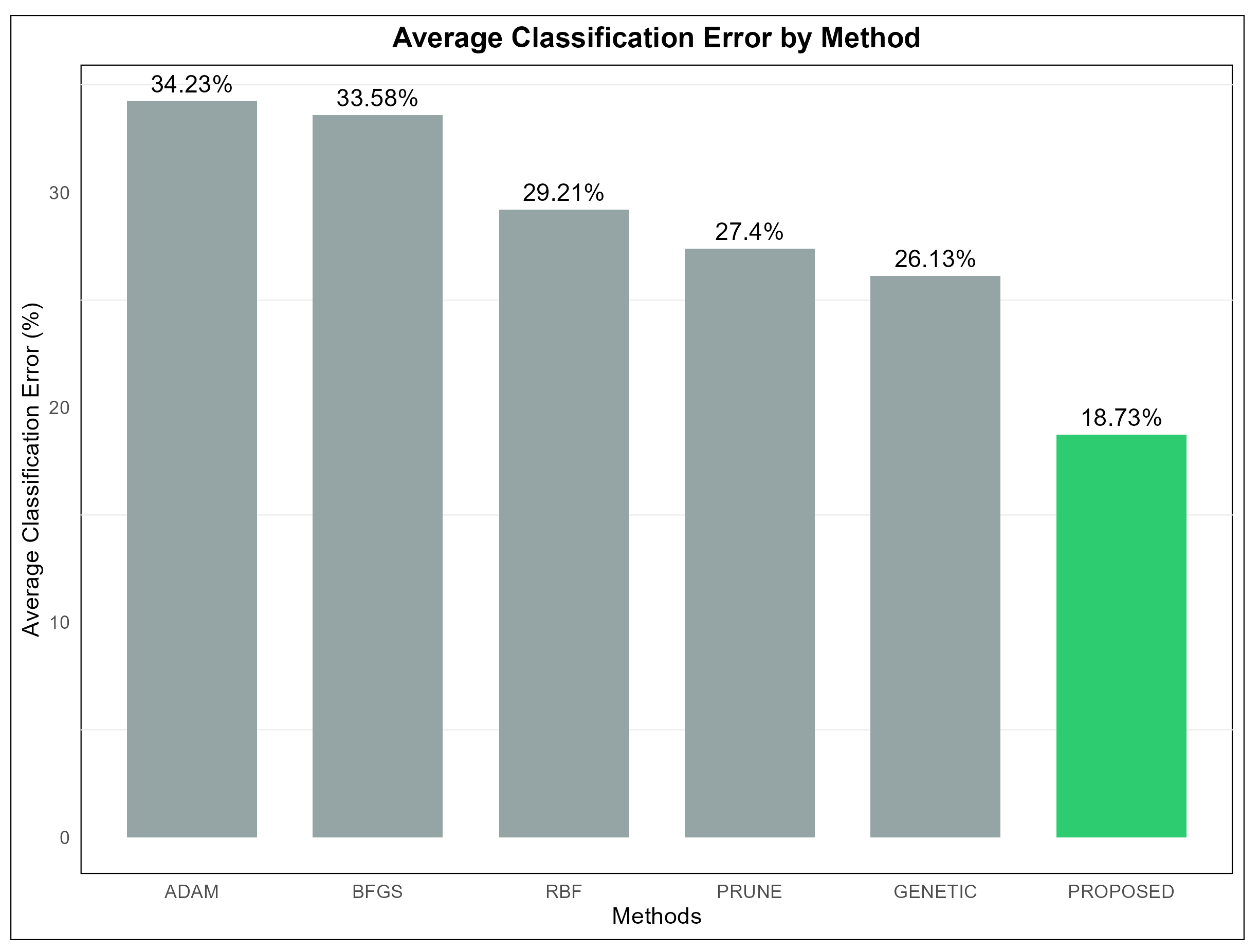
Table 2 presents a detailed comparison of the performance of six different machine learning models, namely ADAM, BFGS, GENETIC, RBF, PRUNE, and PROPOSED, evaluated across multiple classification datasets. The values in the table represent the error rates for each model on each dataset, expressed as percentages. Lower error rates indicate better performance for a given model on a specific dataset. The last row of the table provides the average error rate for each model, serving as a measure of their overall effectiveness across all datasets. From an analysis of this table, it becomes evident that the PROPOSED model achieved the best overall performance, with an average error rate of 18.73%. This was the lowest among all the models evaluated, demonstrating its superior effectiveness in solving classification problems across a diverse set of datasets. In particular, the PROPOSED model consistently outperformed the other models on datasets such as DERMATOLOGY, ZONF_S, and ZOO, where it recorded the smallest error rates, indicating its robustness in handling datasets of varying complexity and characteristics. The GENETIC model, on the other hand, had the highest average error rate at 26.13%, making it the least effective model overall. This result suggests that, while the GENETIC model may perform adequately in certain contexts, it lacks the adaptability and overall reliability exhibited by the PROPOSED model. Examining the ADAM model, we observed an average error rate of 34.23%, which was one of the highest among the models. Despite this, ADAM demonstrated good performance on specific datasets, such as CIRCULAR and SPIRAL, where its error rates were notably low. This indicates that the performance of ADAM is heavily dependent on the structure and features of the datasets, performing well in certain contexts but underperforming in others. Similarly, the BFGS model had an average error rate of 33.58%, slightly lower than ADAM, but it exhibited comparable variability in its performance across datasets. The RBF model, with an average error rate of 29.21%, performed better than both ADAM and BFGS. RBF appeared to be more stable in its performance, achieving lower error rates across a broader range of datasets, although it did not consistently outperform the PROPOSED model. The PRUNE model achieved an average error rate of 27.40%, which placed it between RBF and GENETIC in terms of overall effectiveness. While PRUNE did not outperform the PROPOSED model in most cases, it shows competitive performance on datasets such as GLASS, where it recorded one of the lowest error rates. This highlights that PRUNE can be effective on certain specialized datasets, though it lacks the overall adaptability of the PROPOSED model. A closer inspection of specific datasets further reinforces the dominance of the PROPOSED model. For instance, on the STATHEART and WINE datasets, which are characterized by increased complexity, the PROPOSED model achieved significantly lower error rates compared to the other models, indicating its ability to effectively handle challenging classification tasks. Additionally, on the HOUSEVOTES dataset, the PROPOSED model performed exceptionally well, suggesting its reliability on datasets with distinct structures. The GENETIC model, while generally less effective, demonstrated relatively strong performance on a few datasets, such as HAYES-ROTH and SPIRAL, where its error rates were comparable to or better than those of the other models. However, its overall high average error rate indicates that its performance was inconsistent and heavily dependent on the specific dataset. Similarly, PRUNE performed well on datasets like MAMMOGRAPHIC but fell behind on others, such as SEGMENT and BALANCE, where the PROPOSED model outperformed it by a considerable margin. The results for the BFGS model reveal a mixed performance profile. It achieved relatively low error rates on datasets such as BALANCE and HEART, but it struggled on datasets like CLEVELAND and LIVERDISORDER, where its error rates were higher than most of the other models. This inconsistency highlights the model’s limited generalizability across datasets. In conclusion, the PROPOSED model demonstrated the best overall performance across the majority of the datasets, achieving the lowest average error rate and consistently outperforming the other models in a wide range of contexts. This suggests that the PROPOSED model is highly adaptable and effective, making it suitable for diverse classification tasks. The analysis further underscores the importance of selecting an appropriate model based on the characteristics of the dataset, as models like ADAM, BFGS, and PRUNE showed strong performance in specific scenarios but fell short in others. The average error rate remains a critical indicator for evaluating the overall effectiveness of models, providing valuable insights into their strengths and weaknesses.

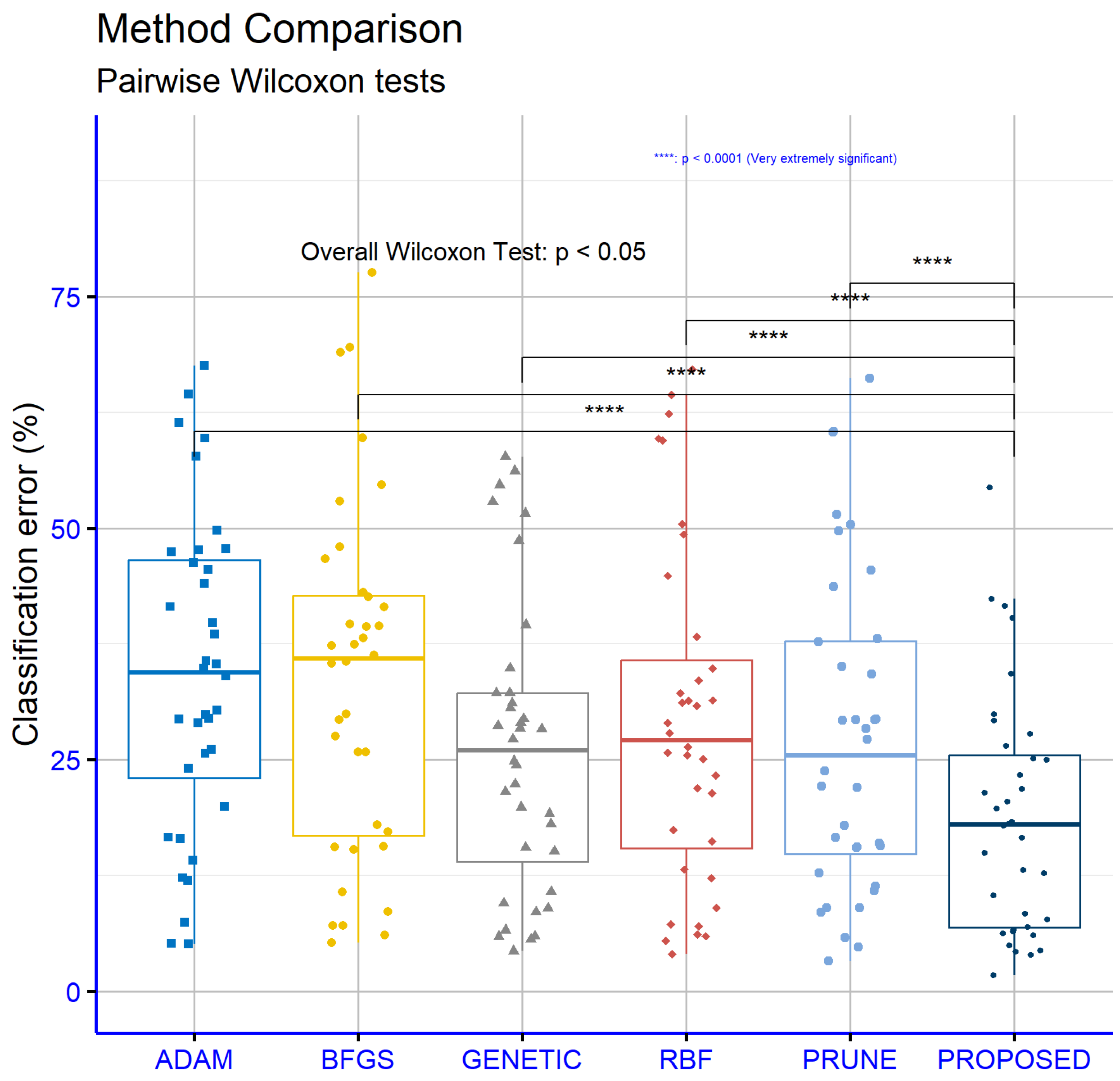
The dynamics of the proposed technique on the classification data are also presented graphically in Figure 3, where the average classification error per method is presented.

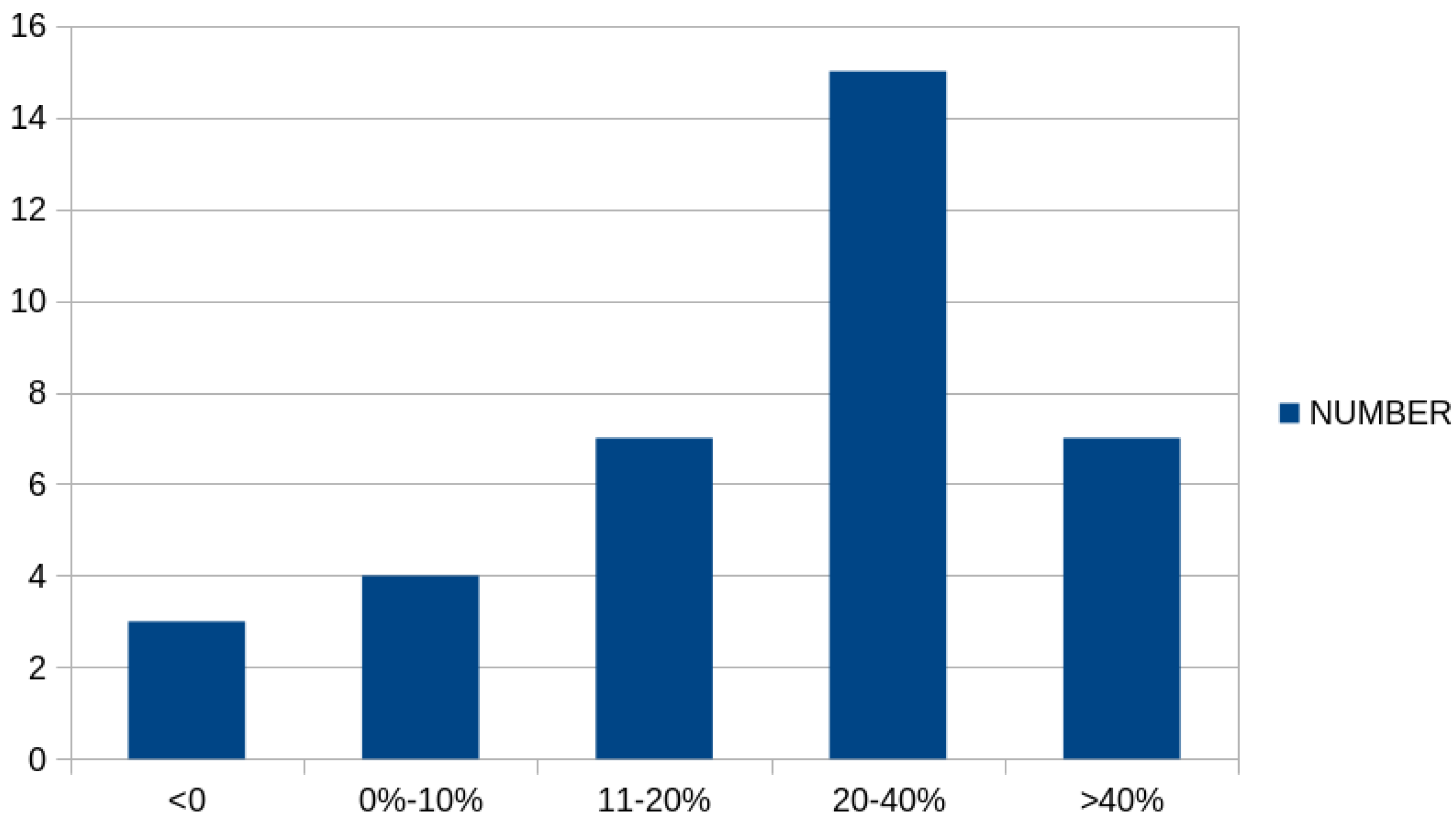
Furthermore, Figure 4 graphically presents the number of cases in which there was a significant reduction in classification error between the simple genetic algorithm and the proposed method. As is evident, in a significant number of cases, there was a drastic reduction in classification error, exceeding 20% or even 40%.

Moreover, a comparison of the factors of precision and recall between the original genetic algorithm and the proposed method is outlined in

Table 4. Comparison of precision and recall between the original genetic algorithm and the proposed method.

	GENETIC		PROPOSED
DATASET	PRECISION	RECALL	PRECISION	RECALL
APPENDICITIS	0.81	0.81	0.86	0.85
ALCOHOL	0.58	0.61	0.83	0.83
AUSTRALIAN	0.67	0.66	0.79	0.80
BALANCE	0.83	0.88	0.86	0.92
CLEVELAND	0.43	0.53	0.45	0.59
CIRCULAR	0.91	0.91	0.94	0.94
DERMATOLOGY	0.72	0.90	0.90	0.88
ECOLI	0.41	0.44	0.54	0.59
GLASS	0.47	0.58	0.48	0.52
HABERMAN	0.61	0.59	0.62	0.61
HAYES ROTH	0.40	0.47	0.70	0.65
HEART	0.70	0.69	0.86	0.85
HEARTATTACK	0.71	0.70	0.77	0.78
HOUSEVOTES	0.91	0.92	0.95	0.96
IONOSPHERE	0.85	0.87	0.90	0.86
LIVERDISORDER	0.69	0.67	0.67	0.66
LYMOGRAPHY	0.68	0.69	0.84	0.85
MAMMOGRAPHIC	0.80	0.80	0.84	0.84
PARKINSONS	0.79	0.68	0.86	0.76
PHONEME	0.79	0.78	0.78	0.76
PIMA	0.65	0.64	0.71	0.70
POPFAILURES	0.80	0.84	0.84	0.83
REGIONS2	0.53	0.63	0.60	0.68
SAHEART	0.62	0.66	0.66	0.63
SEGMENT	0.53	0.50	0.67	0.67
SONAR	0.80	0.78	0.78	0.76
SPIRAL	0.55	0.55	0.56	0.56
STATHEART	0.70	0.70	0.81	0.80
STUDENT	0.96	0.96	0.96	0.96
TRANSFUSION	0.69	0.68	0.68	0.63
WDBC	0.92	0.90	0.94	0.93
WINE	0.78	0.86	0.95	0.93
Z_F_S	0.90	0.88	0.92	0.92
ZO_NF_S	0.78	0.78	0.94	0.94
ZOO	0.90	0.90	0.94	0.96
AVERAGE	0.71	0.73	0.78	0.78

for the classification datasets.

Similarly, Table 3 presents a comparison of the performance of the same machine learning models, across a series of regression datasets. The values in the table are absolute and represent the error of each model for each dataset. From the analysis, it is evident that the proposed model (PROPOSED) demonstrated the best overall performance, with an average error of 5.23. This value is significantly lower than the average errors of the other models, highlighting that PROPOSED was the most effective model for regression problems. The GENETIC model exhibited the second-lowest average error, 9.31, indicating that it is also a reliable choice, though noticeably less effective than PROPOSED. The RBF model achieved an average error of 10.02, ranking third in performance, while showing consistent results across many datasets. The PRUNE model had an average error of 15.4, which is higher than GENETIC and RBF, but it still showed remarkable performance on specific datasets, such as CONCRETE and LASER. The ADAM and BFGS models had the highest average errors, 22.46 and 30.29, respectively, making them the least effective overall. At the individual dataset level, the PROPOSED model demonstrated superior performance in many instances. For example, on the AIRFOIL, CONCRETE, LASER, and MORTGAGE datasets, PROPOSED recorded the smallest error values, underscoring its high effectiveness in addressing problems with varying characteristics. On the BL dataset, the PROPOSED model achieved an exceptionally low error of 0.006, the smallest among all models. On more complex datasets, such as BASEBALL and HOUSING, PROPOSED significantly outperformed the other models, with error values of 60.74 and 20.74, respectively. These results emphasize its adaptability to problems with different levels of complexity. The GENETIC model, while performing well overall, showed significant variability. For instance, it recorded relatively low errors on the AUTO and PLASTIC datasets, with values of 12.18 and 2.791, respectively, but exhibited considerably higher errors on others, such as STOCK and BASEBALL. This inconsistency suggests limited stability. Similarly, the RBF model demonstrated good overall performance, with notable results on datasets like MORTGAGE and PL, where its errors were among the lowest. However, on datasets like AUTO and STOCK, its errors were significantly higher than those of the PROPOSED model. The PRUNE model delivered noteworthy results on specific datasets. For example, on CONCRETE, it achieved one of the smallest errors, only 0.0077, while on datasets such as PLASTIC and TREASURY, its error was larger, indicating less consistency under varying conditions. On the other hand, ADAM, despite being generally less effective, performed well on a few datasets like BK and QUAKE, where it recorded lower errors compared to the other models. The BFGS model, with the highest average error, consistently underperformed across most datasets, with standout poor results on BASEBALL and STOCK, where it records particularly high error values. In summary, an analysis of the table reveals that the proposed model, PROPOSED, achieved the best overall performance compared to the other models, while being particularly effective on datasets with varying levels of complexity. The average error serves as a useful indicator of the effectiveness of each model, reaffirming the superiority of the PROPOSED model across a wide range of regression problems.

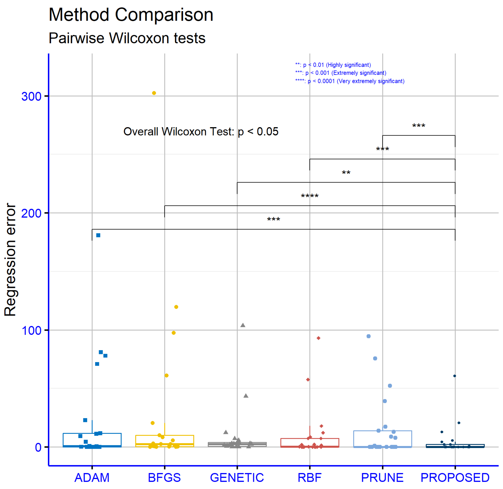
Figure 5 focuses on regression datasets and reveals similar results favoring the proposed model, although the “p” values are slightly higher compared to those in the classification datasets. The comparison between PROPOSED and ADAM produced a “p” value of 0.0001, indicating a statistically significant difference in favor of the PROPOSED model. Comparisons with the other models, specifically PROPOSED vs. BFGS (p = 4.1 × 10⁻⁵), PROPOSED vs. GENETIC (p = 0.0022), PROPOSED vs. RBF (p = 0.00073), and PROPOSED vs. PRUNE (p = 0.00042), also demonstrated statistically significant differences. All “p” values remained below the 0.05 threshold, affirming that the observed performance differences are not attributable to randomness. Notably, the very low “p” values on the regression datasets underscore the overall effectiveness of the PROPOSED model in addressing regression problems. The PROPOSED model demonstrated a high level of adaptability across various datasets with diverse characteristics, consistently maintaining its superiority over the other models.

Consequently, the results from Figure 6 further strengthen the position of the PROPOSED model as the most effective solution for regression problems, providing a reliable and statistically significant performance.

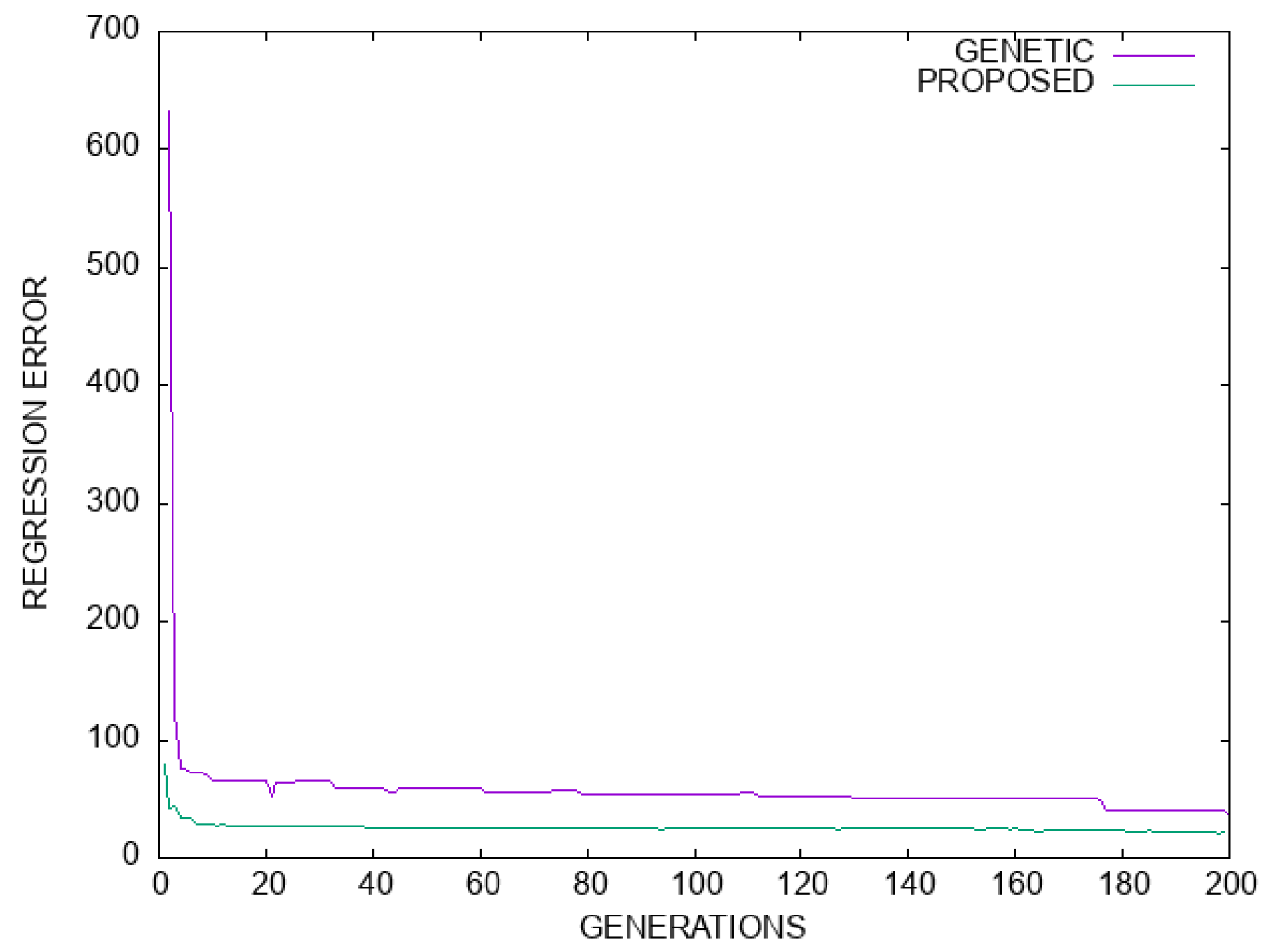
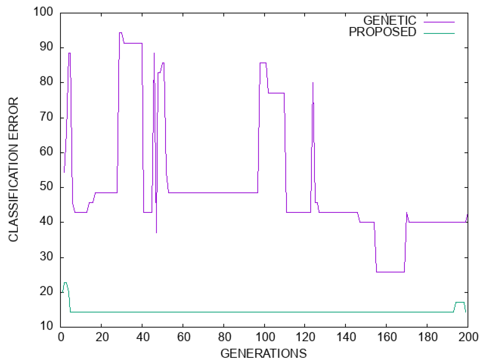
Moreover, in the plot of Figure 7 a comparison in terms of classification error is made between the simple genetic algorithm and the proposed model for the Dermatology dataset. Likewise, in Figure 8 a plot of the regression error is outlined for the genetic algorithm and the proposed method. For both cases, there is a significant improvement in terms of error values.

3.2. Using Different Weight Methods

An additional experiment was executed, where the parameter F of the differential evolution was altered using some well-known approaches from the relevant literature. In the following tables, the following methods, as denoted in the experimental tables, were used for the calculation of the parameter F:

• RANDOM. This method was used for the current approach, where the differential weight is a random number in $[0, 1]$.
• FIXED. This method was used when the value for F was used, as denoted in Table 1.
• ADAPT. This method was used for the adaptive calculation of parameter F, as proposed in [89].
• MIGRANT. For this case, the calculation for parameter F as proposed in [90] was adopted.

The experimental results using the current method and the previously mentioned method for differential weight are listed in

Table 5. Experimental results for the classification datasets and the proposed method using a series of differential weight mechanisms.

DATASET	RANDOM	FIXED	ADAPT	MIGRANT
APPENDICITIS	15.00%	14.90%	15.30%	15.80%
ALCOHOL	18.33%	20.81%	22.08%	17.26%
AUSTRALIAN	21.49%	19.62%	23.91%	29.49%
BALANCE	7.79%	7.56%	8.39%	8.39%
CLEVELAND	42.38%	42.31%	41.79%	44.79%
CIRCULAR	6.50%	7.24%	7.40%	4.74%
DERMATOLOGY	4.97%	5.72%	5.71%	11.40%
ECOLI	40.30%	42.18%	45.51%	47.61%
GLASS	54.38%	54.33%	56.29%	49.00%
HABERMAN	26.53%	27.93%	30.00%	26.60%
HAYES-ROTH	34.31%	34.00%	28.62%	35.00%
HEART	13.11%	15.30%	14.56%	19.04%
HEARTATTACK	21.90%	19.57%	20.00%	20.70%
HOUSEVOTES	6.09%	6.00%	5.22%	5.48%
IONOSPHERE	10.37%	9.71%	8.86%	11.80%
LIVERDISORDER	29.94%	30.97%	29.56%	31.12%
LYMOGRAPHY	17.93%	18.93%	20.72%	20.93%
MAMMOGRAPHIC	16.63%	15.74%	16.12%	17.50%
PARKINSONS	12.79%	9.69%	11.58%	14.42%
PHONEME	18.10%	17.23%	18.15%	18.40%
PIMA	25.03%	27.66%	27.89%	27.70%
POPFAILURES	4.45%	5.19%	4.82%	4.39%
REGIONS2	25.19%	25.03%	23.24%	30.92%
SAHEART	29.26%	32.26%	30.76%	32.28%
SEGMENT	27.80%	36.29%	33.83%	42.80%
SONAR	20.50%	20.85%	21.00%	22.10%
SPIRAL	41.60%	43.93%	45.67%	44.04%
STATHEART	19.74%	18.52%	16.67%	17.41%
STUDENT	4.00%	4.38%	4.25%	4.63%
TRANSFUSION	23.35%	22.95%	24.58%	23.50%
WDBC	6.73%	6.48%	7.50%	4.18%
WINE	6.29%	5.82%	6.35%	11.59%
Z_F_S	8.38%	7.00%	9.27%	10.43%
ZO_NF_S	4.32%	5.52%	6.00%	8.36%
ZONF_S	1.76%	1.92%	2.20%	2.32%
ZOO	7.00%	4.90%	9.00%	6.10%
AVERAGE	18.73%	19.12%	19.52%	20.62%

and

Table 6. Experimental results for the regression datasets and the proposed method using a variety of techniques for the calculation of differential weight.

DATASET	RANDOM	FIXED	ADAPT	MIGRANT
ABALONE	4.32	4.47	4.35	4.41
AIRFOIL	0.002	0.003	0.003	0.003
AUTO	12.78	13.58	13.98	11.46
BK	0.02	0.057	0.021	0.021
BL	0.006	0.008	0.006	0.008
BASEBALL	60.74	65.12	67.71	60.10
CONCRETE	0.006	0.026	0.007	0.004
DEE	0.19	0.21	0.20	0.24
FRIEDMAN	2.21	2.79	3.18	1.88
FY	0.067	0.046	0.042	0.052
HO	0.015	0.017	0.052	0.013
HOUSING	20.74	24.63	24.83	24.71
LASER	0.004	0.004	0.004	0.003
LW	0.011	0.014	0.011	0.013
MORTGAGE	0.32	0.71	0.32	0.22
PL	0.022	0.022	0.022	0.023
PLASTIC	2.16	2.15	2.15	2.36
QUAKE	0.036	0.052	0.036	0.044
SN	0.023	0.036	0.025	0.024
STOCK	5.57	5.89	4.72	4.41
TREASURY	0.68	0.64	0.51	0.65
AVERAGE	5.23	5.74	5.82	5.27

for the classification datasets and the regression datasets, respectively.

Figure 8. Comparison between the genetic algorithm and the proposed method for the Housing regression dataset. The horizontal axis denotes the number of generations, and the vertical axis gives the regression error as measured on the test set.

Figure 8. Comparison between the genetic algorithm and the proposed method for the Housing regression dataset. The horizontal axis denotes the number of generations, and the vertical axis gives the regression error as measured on the test set.

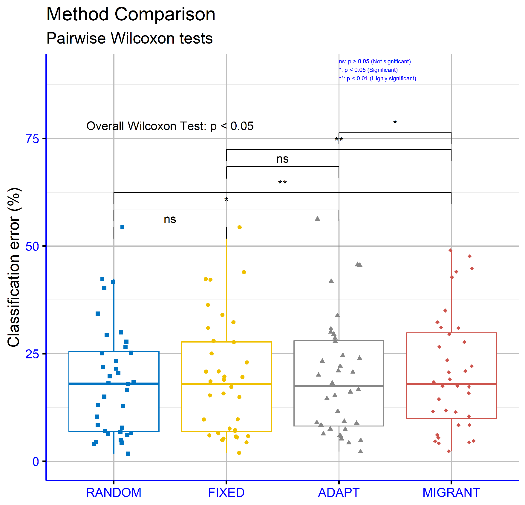
The statistical analysis in Table 5 examines the percentage error rates across various classification datasets using four different computations of the critical weight differential parameter for the proposed machine learning model: RANDOM, FIXED, ADAPT, and MIGRANT. The RANDOM computation exhibited the lowest overall average error rate (18.73%), indicating superior performance compared to the other computations: FIXED (19.12%), ADAPT (19.52%), and MIGRANT (20.62%). This suggests that the RANDOM computation was the most reliable overall. Analyzing individual datasets, the RANDOM computation achieved the best error rates in several cases. For instance, it recorded the lowest error rates for datasets such as “ALCOHOL” (18.33%), “BALANCE” (7.79%), “CIRCULAR” (6.50%), “HOUSEVOTES” (6.09%), “PARKINSONS” (12.79%), “POPFAILURES” (4.45%), and “WDBC” (6.73%). These results highlight its effectiveness across a wide range of datasets. Specifically, the 4.45% error rate for “POPFAILURES” stands out as one of the lowest overall. In certain datasets, the FIXED computation outperformed the others, such as on “Z_F_S” (7.00%) and “ZOO” (4.90%). However, the difference from RANDOM is minimal. The MIGRANT computation demonstrated the lowest error rates in only a few cases, such as “CIRCULAR” (4.74%) and “WDBC” (4.18%), suggesting it may be particularly effective for specific datasets. Meanwhile, the ADAPT computation achieved lower error rates on a few scenarios but generally remained less competitive. On other datasets, such as “GLASS”, “SPIRAL”, and “SEGMENT”, all computations showed high error rates, indicating that these datasets are challenging to classify, regardless of the computation. Nevertheless, the RANDOM computation remained consistently competitive, even with these difficult datasets, as observed on “STATHEART” and “ZONF_S”. In conclusion, the analysis revealed that the RANDOM computation was the most effective overall, achieving the lowest average error rate and demonstrating superior performance across a broad range of datasets. However, there were instances where other computations, such as FIXED and MIGRANT, showed specialized advantages.

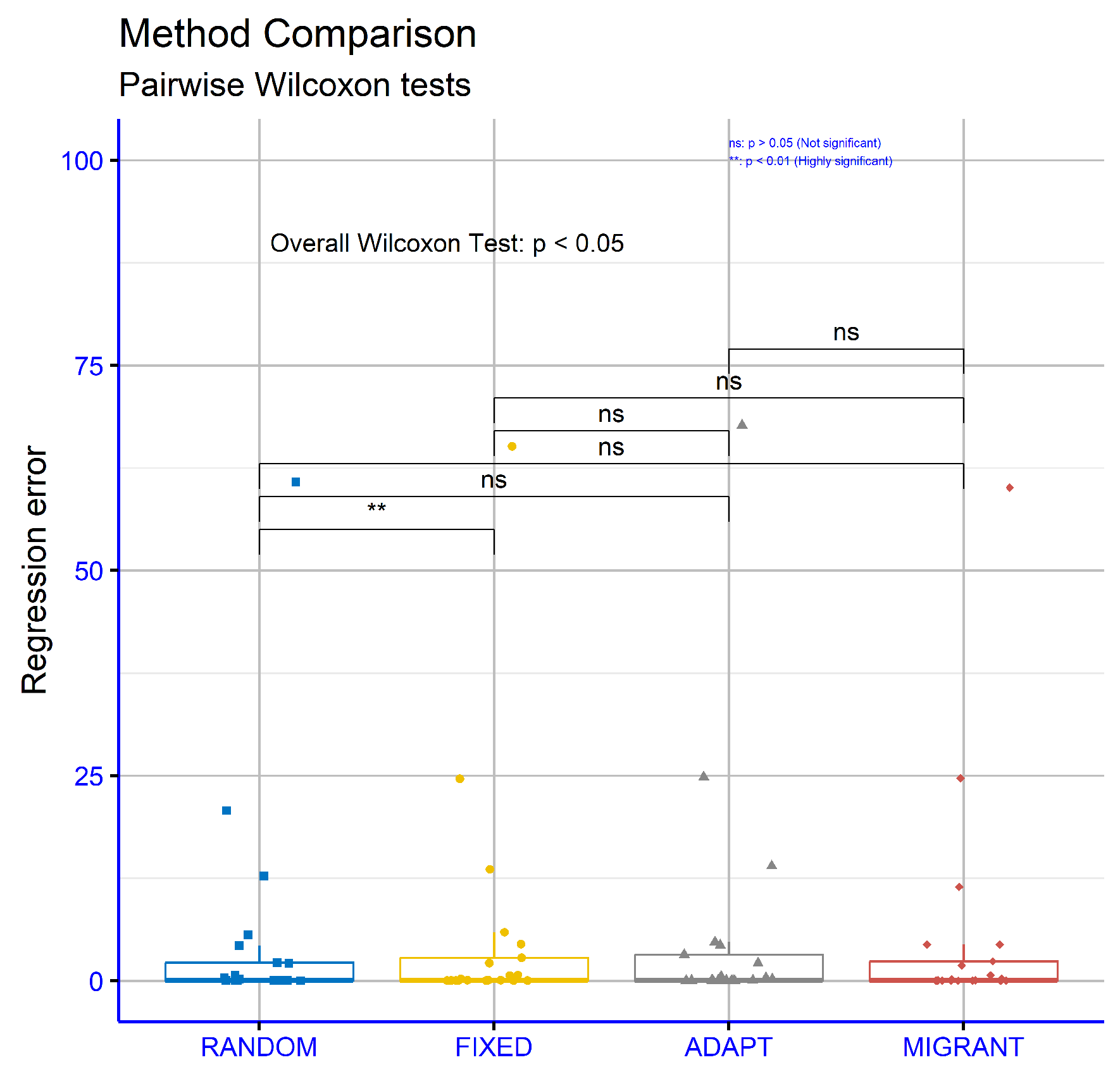
The statistical analysis in Table 6 pertains to regression datasets, using four different calculations of the critical parameter of differential weighting for the proposed machine learning model: RANDOM, FIXED, ADAPT, and MIGRANT. The RANDOM calculation exhibited the lowest average error (5.23), making it the most efficient overall compared to FIXED (5.74), ADAPT (5.82), and MIGRANT (5.27). The small difference between RANDOM and MIGRANT suggests a comparable performance between these two approaches, with RANDOM maintaining a slight edge. For individual datasets, the RANDOM calculation achieved the lowest error values in several cases, such as the “AUTO” (12.78), “FRIEDMAN” (2.21), “HO” (0.015), “MORTGAGE” (0.32), and “SN” (0.023) datasets. These results demonstrate the effectiveness of the RANDOM calculation across a wide range of datasets. On the “FRIEDMAN” dataset, the error value of 2.21 was significantly lower than the corresponding values of FIXED (2.79) and ADAPT (3.18), underscoring its performance on this specific dataset. The MIGRANT calculation demonstrated the best performance on certain datasets, such as “AUTO” (11.46) and “STOCK” (4.41), where it outperformed RANDOM. However, on other datasets, such as “PLASTIC” and “SN”, it showed slightly higher error rates, indicating limitations with specific data. The FIXED calculation tended to have consistent but not top-performing results, while ADAPT generally showed higher error values, making it less effective overall. In summary, the analysis highlighted that the RANDOM calculation was the most reliable and efficient, with the lowest average error and strong performance across various datasets. However, the MIGRANT calculation exhibited competitive performance in specific cases, while FIXED and ADAPT appear to require improvements to rival the other calculations.

Figure 9 evaluates the classification datasets for different differential weight computations within the proposed machine learning model. The p-values are as follows: RANDOM vs. FIXED: p = 0.43, RANDOM vs. ADAPT: p = 0.024, RANDOM vs. MIGRANT: p = 0.0021, FIXED vs. ADAPT p = 0.12, FIXED vs. MIGRANT: p = 0.0033, and ADAPT vs. MIGRANT: p = 0.043. These results suggest that some comparisons, such as RANDOM vs. MIGRANT and FIXED vs MIGRANT, showed strong statistical significance, while others, such as RANDOM vs FIXED, did not demonstrate significant differences.

Figure 10 presents the results for regression datasets using different differential weight computations within the proposed model. The observed p-values were RANDOM vs. FIXED: p = 0.0066, RANDOM vs ADAPT: p = 0.15, RANDOM vs. MIGRANT: p = 0.66, FIXED vs. ADAPT: p = 0.64, FIXED vs. MIGRANT: p = 0.84, and ADAPT vs. MIGRANT: p = 0.47. These findings indicate that most comparisons did not show significant differences, except for RANDOM vs. FIXED, which demonstrated a notable level of significance.

3.3. Experiment with the Number of Agents

An additional experiment was conducted using different values for the parameter NP, which represents the number of agents. In this experiment, the parameter NP took the values 50, 100, and 200. The experimental results for the classification datasets are shown in

Table 7. Experimental results for the classification datasets and the proposed method using a variety of values for the parameter NP.

DATASET	NP = 50	NP = 100	NP = 200
APPENDICITIS	14.00%	14.00%	15.00%
ALCOHOL	26.90%	25.36%	18.33%
AUSTRALIAN	30.67%	25.83%	21.49%
BALANCE	7.42%	8.13%	7.79%
CLEVELAND	39.55%	42.10%	42.38%
CIRCULAR	8.50%	6.79%	6.50%
DERMATOLOGY	9.89%	11.34%	4.97%
ECOLI	44.58%	41.48%	40.30%
GLASS	53.24%	55.00%	54.38%
HABERMAN	27.67%	27.70%	26.53%
HAYES-ROTH	36.08%	34.69%	34.31%
HEART	14.89%	14.85%	13.11%
HEARTATTACK	20.73%	17.93%	21.90%
HOUSEVOTES	3.91%	5.22%	6.09%
IONOSPHERE	8.03%	10.43%	10.37%
LIVERDISORDER	32.21%	30.18%	29.94%
LYMOGRAPHY	19.93%	18.86%	17.93%
MAMMOGRAPHIC	15.76%	16.53%	16.63%
PARKINSONS	12.05%	11.63%	12.79%
PHONEME	19.06%	19.08%	18.10%
PIMA	25.75%	28.51%	25.03%
POPFAILURES	5.74%	4.07%	4.45%
REGIONS2	24.71%	24.60%	25.19%
SAHEART	32.33%	31.72%	29.26%
SEGMENT	46.73%	44.27%	27.80%
SONAR	21.95%	22.75%	20.50%
SPIRAL	43.55%	44.08%	41.60%
STATHEART	18.70%	17.67%	19.74%
STUDENT	3.50%	3.70%	4.00%
TRANSFUSION	23.83%	23.87%	23.35%
WDBC	8.82%	7.00%	6.73%
WINE	8.82%	7.12%	6.29%
Z_F_S	8.30%	6.73%	8.38%
ZO_NF_S	7.04%	6.30%	4.32%
ZONF_S	2.08%	2.18%	1.76%
ZOO	6.00%	6.00%	7.00%
AVERAGE	20.36%	19.94%	18.73%

and for the regression datasets in

Table 8. Experimental results for the regression datasets using the proposed method and a variety of values for parameter NP.

DATASET	NP = 50	NP = 100	NP = 200
ABALONE	4.41	4.35	4.32
AIRFOIL	0.003	0.003	0.002
AUTO	14.73	13.63	12.78
BK	0.019	0.018	0.02
BL	0.011	0.009	0.006
BASEBALL	63.75	57.75	60.74
CONCRETE	0.007	0.006	0.006
DEE	0.21	0.20	0.19
FRIEDMAN	3.43	2.83	2.21
FY	0.047	0.041	0.067
HO	0.016	0.014	0.015
HOUSING	28.28	25.95	20.74
LASER	0.005	0.005	0.004
LW	0.01	0.012	0.011
MORTGAGE	0.34	0.48	0.32
PL	0.022	0.022	0.022
PLASTIC	2.16	2.16	2.16
QUAKE	0.037	0.054	0.036
SN	0.026	0.025	0.023
STOCK	5.30	6.34	5.57
TREASURY	1.50	1.16	0.68
AVERAGE	5.92	5.48	5.23

.

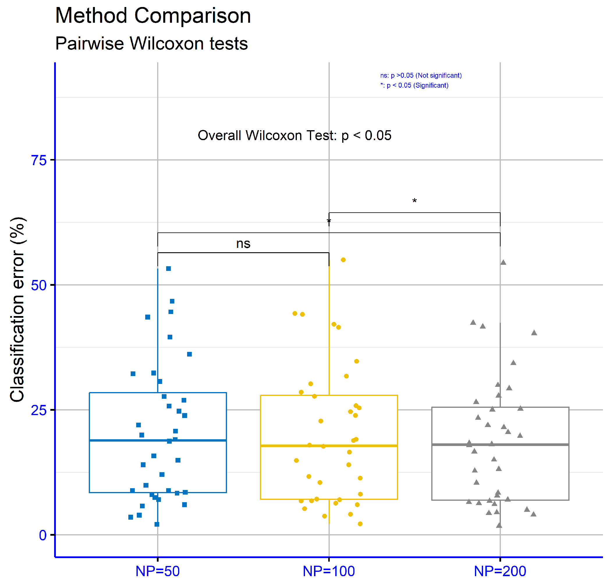
The statistical analysis in Table 7 pertains to classification datasets, utilizing three different values for the critical parameter “NP” in the proposed machine learning model: NP = 50, NP = 100, and NP = 200. The computation with NP = 200 demonstrated the lowest average error rate (18.73%), indicating the highest efficiency compared to NP = 100 (19.94%) and NP = 50 (20.36%). This suggests that a higher value of the NP parameter was generally associated with better performance. On individual datasets, the computation with NP = 200 achieved the lowest error rate in many cases, such as in “ALCOHOL” (18.33%), “AUSTRALIAN” (21.49%), “BALANCE” (7.79%), “DERMATOLOGY” (4.97%), “ECOLI” (40.30%), and “HEART” (13.11%). On some of these datasets, the difference between NP = 200 and the other two values was notable. For instance, on the “DERMATOLOGY” dataset, the error rate with NP = 200 (4.97%) was significantly lower than the corresponding values for NP = 50 (9.89%) and NP = 100 (11.34%), highlighting the clear superiority of NP = 200 for this dataset. However, there were also datasets where the differences were less pronounced. For example, on “PHONEME”, the error rates were relatively close across all parameter values, with NP = 200 showing the smallest error (18.10%). On some other datasets, such as “HOUSEVOTES”, NP = 50 had a lower error rate (3.91%) than the other two parameter values. This indicates that, on certain datasets, increasing the NP parameter did not necessarily lead to improved performance. Similarly, on the “Z_F_S” dataset, NP = 100 achieved the lowest error rate (6.73%), while NP = 200 exhibited a higher rate (8.38%), suggesting that performance may also depend on the characteristics of the data. Despite these exceptions, NP = 200 generally exhibited the best overall performance, achieving the lowest average error rate and delivering strong results across a wide range of datasets.

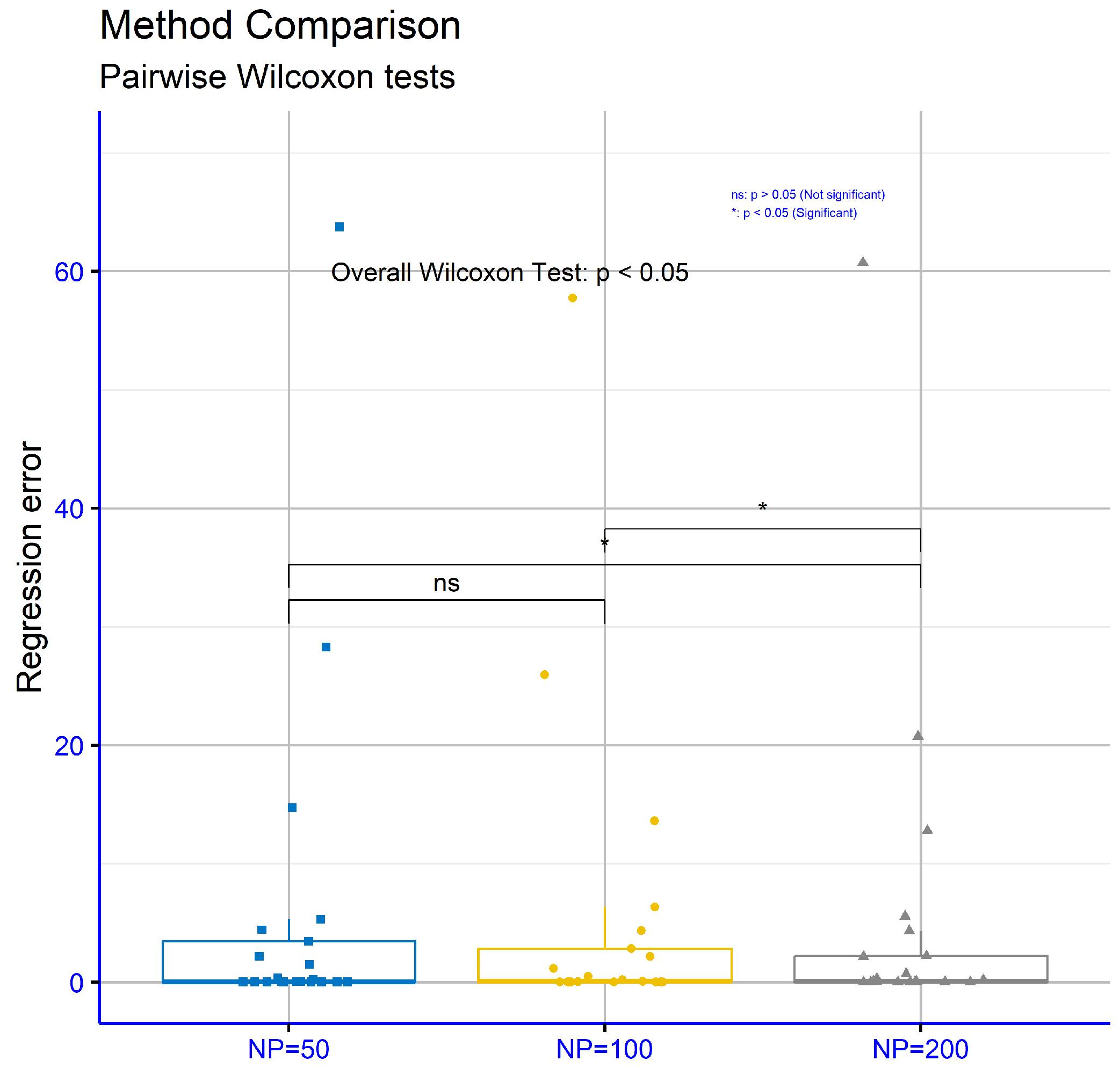
The analysis in Table 8 focuses on regression datasets, considering three distinct values for the critical parameter “NP” in the proposed machine learning model: NP = 50, NP = 100, and NP = 200. The parameter NP = 200 achieved the lowest average error (5.23), making it more effective than NP = 100 (5.48) and NP = 50 (5.92). This suggests that higher NP values are generally associated with improved performance. On specific datasets, NP = 200 stood out for its superior performance. For instance, on “AIRFOIL” (0.002), “AUTO” (12.78), “BL” (0.006), “CONCRETE” (0.006), “FRIEDMAN” (2.21), and “TREASURY” (0.68), the error values for NP = 200 were the lowest. On the “FRIEDMAN” dataset, NP = 200 (2.21) significantly outperformed NP = 50 (3.43) and NP = 100 (2.83), demonstrating its effectiveness. However, there were cases where other NP values showed stronger performance. For example, on the “BK” dataset, NP = 100 achieved the lowest error (0.018), while NP = 200 (0.02) was slightly worse. Similarly, on the “FY” dataset, NP = 100 exhibited the best performance (0.041), with NP = 200 showing a higher error (0.067). Additionally, on the “BASEBALL” dataset, NP = 100 outperformed NP =2 00, recording an error of 57.75 compared to 60.74. These variations indicate that the effectiveness of the NP parameter can depend on the characteristics of the dataset. Overall, NP = 200 demonstrated the best average performance, highlighting its value in most cases. While the other NP values achieved lower error rates on some datasets, NP = 200 stood out for its general reliability and efficiency.

In Figure 11, focusing on classification datasets for different values of the critical parameter “NP” within the proposed model, the p-values are NP = 50 vs. NP = 100: p = 0.17, NP = 50 vs. NP = 200: p = 0.117, and NP = 100 vs. NP = 200: p = 0.032. These results indicate that only the comparison between NP = 100 and NP = 200 demonstrated statistical significance.

Finally, Figure 12 evaluates regression datasets for different values of the critical parameter “NP” within the proposed model. The respective p-values are NP = 50 vs. NP = 100: p = 0.08, NP = 50 vs. NP = 200: p = 0.012, and NP = 100 vs NP = 200: p = 0.025. These results show that the comparisons NP = 50 vs. NP = 200 and NP = 100 vs. NP = 200 exhibited statistically significant differences, while the comparison NP = 50 vs. NP = 100 did not.

3.4. Discussion

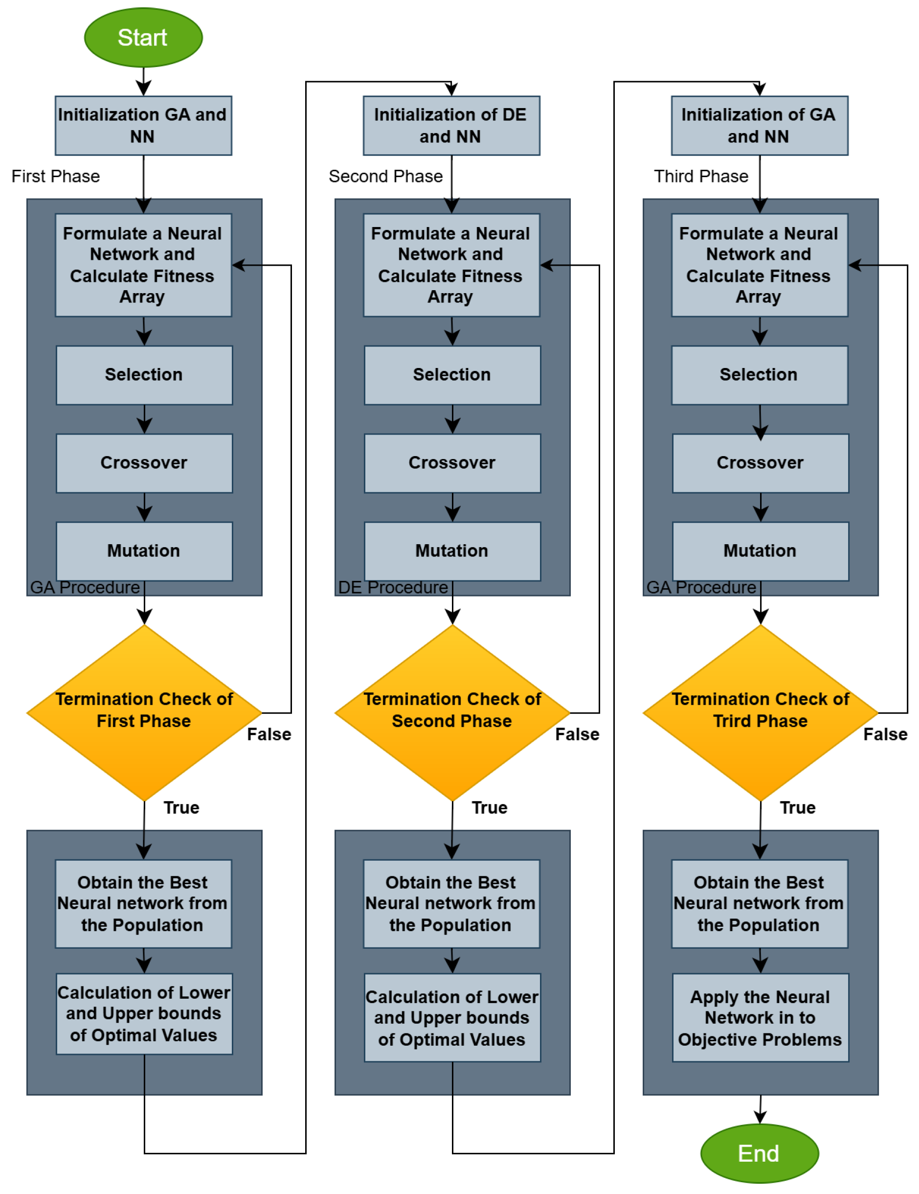
This study introduced an innovative three-stage evolutionary method for training artificial neural networks (ANNs), with the primary goal of reducing both training error and overfitting. The results show that the proposed approach achieved a mean classification error of 18.73% and a mean regression error of 5.23, significantly outperforming conventional methods such as ADAM, BFGS, PRUNE, genetic algorithms, and radial basis function (RBF) networks. This improvement demonstrates that combining genetic algorithms with differential evolution to define optimal parameter bounds is an effective strategy for enhancing model generalization. Specifically, the use of a modified fitness function, which penalizes large deviations in weight values, appeared to limit the networks’ tendency to overfit training data. For example, on datasets like “DERMATOLOGY”, where the classification error dropped to 4.97%, the method maintained high accuracy, even in cases of high variability.

Compared to previous studies that focused on standalone techniques like genetic-algorithm-based training or Adam optimizers, the current method introduces two critical innovations. First, the differential evolution in the second stage enables systematic exploration of the parameter space to identify optimal value intervals for weights. Second, the multi-stage nature of the process initial boundary estimation, interval optimization, and final training provides a structured framework for managing problem complexity. These enhancements explain the significant reduction in mean error compared to prior methods, such as the decrease from 26.13% to 18.73% in classification and from 10.02 to 5.23 in regression.

However, the method is not without limitations. A primary constraint is its high computational cost, stemming from the three-stage process and the large number of agents (NP = 200) required to explore the parameter space. Additionally, the method’s performance heavily depends on hyperparameter tuning, such as crossover probability (CR). For instance, on datasets like “SEGMENT” (27.80% error) or “STOCK” (5.57 error), the method showed relative weakness, likely due to data complexity or noise. Furthermore, the use of a single hidden layer (H = 10) may be insufficient for high-dimensional problems, highlighting the need for more complex architectures.

Error sources can be attributed to multiple factors. On medical datasets like “CLEVELAND” (42.38% error), noise or class imbalance may have affected accuracy. Additionally, the random weight initialization in the first stage can lead to suboptimal solutions, while the network’s static architecture limits its ability to handle non-linear relationships. However, a clear trend emerged: increasing the number of agents (NP) improves performance, as seen in the reduction in mean classification error from 20.36% (NP = 50) to 18.73% (NP = 200). This suggests that a broader parameter space exploration enhances generalization.

4. Conclusions

The proposed evolutionary method, based on differential evolution, proved highly effective in optimizing the weights of artificial neural networks, significantly reducing both the training error and overfitting. Compared to other popular methods such as ADAM, BFGS, PRUNE genetic algorithms, and radial basis function (RBF) networks, the new approach demonstrated superior performance in classification tasks, with a mean error of 18.73%, and regression tasks, with a mean error of 5.23%. Despite these positive results, certain datasets, such as “SEGMENT” and “STOCK”, exhibited higher errors, likely due to data complexity or inherent noise affecting the prediction accuracy. The random computation of parameter F and the use of a larger number of agents (e.g., NP = 200) enhanced system performance. However, smaller NP values yielded better results in some cases, highlighting the need for adaptive parameter tuning mechanisms during optimization.

The significance of this research lies in the method’s ability to address two critical challenges in machine learning: reducing training error, and controlling overfitting. By sequentially using genetic algorithms for the initial boundary definition, differential evolution for interval optimization, and a final training phase, the method provides a structured framework that enhances model generalization. This makes it particularly useful in applications where reliability and interpretability are critical, such as medical diagnosis or industrial failure prediction. For example, the exceptional performance on the “DERMATOLOGY” dataset (4.97% error) demonstrates its robustness, even under high-variance conditions.

However, the method operates within specific constraints. High computational costs, due to the three-stage process and large number of agents, limit its applicability in real-time or resource-constrained environments. Additionally, its performance heavily depends on manual hyperparameter tuning, such as crossover probability (CR). Furthermore, the use of simple architectures with a single hidden layer (H=10) restricts its ability to model complex relationships, as seen in the underperformance on datasets like “SEGMENT” (27.80% error). Noise in the data or class imbalance, as in “CLEVELAND” (42.38% error), can worsen results, emphasizing the need for preprocessing or domain-specific adaptations.

For future research, developing mechanisms for dynamic parameter tuning (e.g., automated selection of CR or NP) is essential to reduce reliance on manual experimentation. Applying the method to high-dimensional data, such as images or text, would help evaluate its flexibility in domains like computer vision or natural language processing. Combining it with techniques like reinforcement learning or attention mechanisms could improve adaptability in dynamic environments. Finally, a theoretical analysis of the algorithm’s convergence and stability, alongside empirical studies on underperforming datasets, could isolate error sources (e.g., noise sensitivity) and lead to optimizations.

In practical terms, the method is highly relevant in domains where generalization and interpretability outweigh speed, such as healthcare or critical infrastructure systems. However, its current weaknesses necessitate cautious application in resource-limited or highly complex scenarios. With strategic improvements in dynamic tuning and integration with advanced architectures, the method could become a cornerstone tool for next-generation neural networks, balancing theoretical innovation and practical utility.

A key problem of the new technique is the slow training times of artificial neural networks, since it is a three-stage technique. In each stage, a separate stochastic technique must be applied. This means that the execution time will be increased compared to other techniques, such as the simple genetic algorithm. Of course, some individual parts of the process could be accelerated by using parallel computing techniques. Finally, although the method uses a genetic algorithm in its last stage to evaluate the parameter value ranges, other optimization techniques could be used in its place, such as the Differential Evolution technique and the PSO technique.