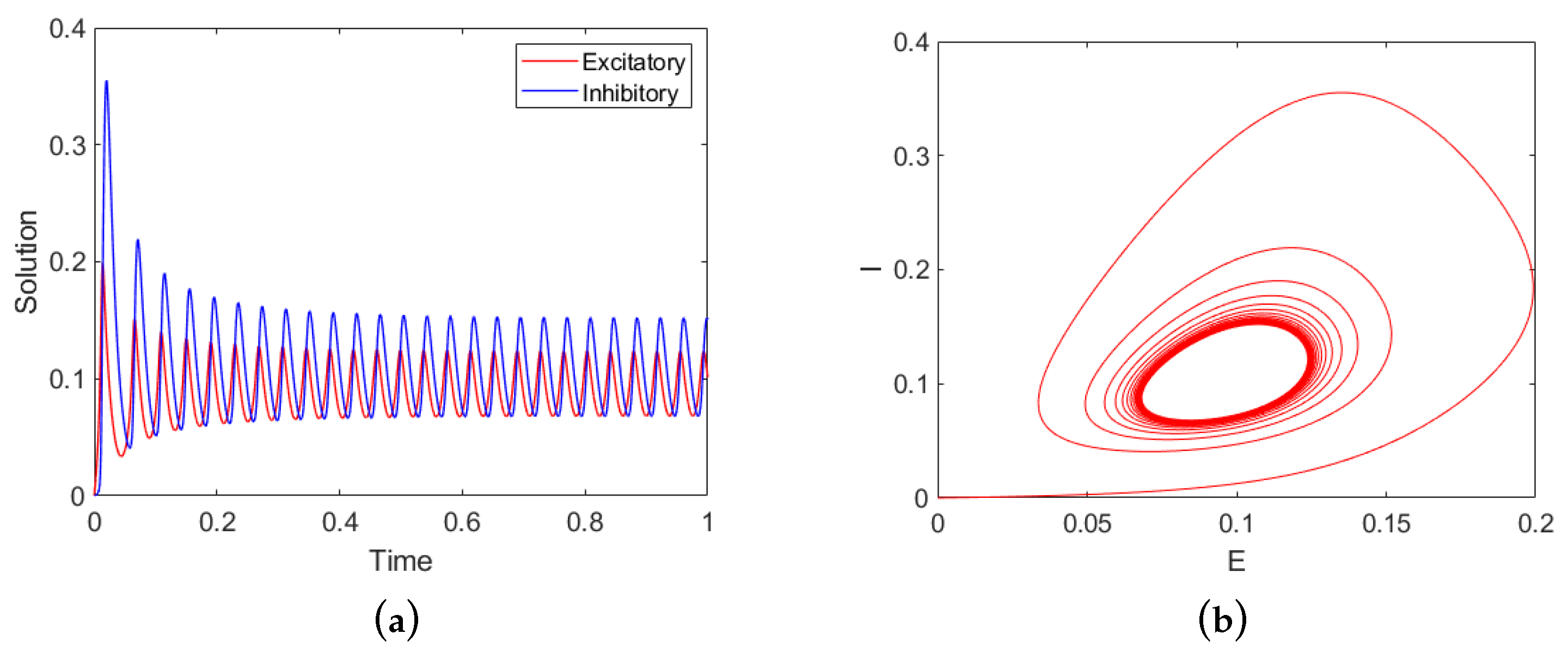
Figure 1.
Numerical solution of the Wilson–Cowan Equations (
1) and (
2). (
a) Time course of the excitatory (red curve) and the inhibitory (blue curve) neuron populations. (
b) The excitatory-inhibitory (
E-
I) phase plane plot. Parameters:
,
,
, and
C is given in Equation (
67).
Figure 1.
Numerical solution of the Wilson–Cowan Equations (
1) and (
2). (
a) Time course of the excitatory (red curve) and the inhibitory (blue curve) neuron populations. (
b) The excitatory-inhibitory (
E-
I) phase plane plot. Parameters:
,
,
, and
C is given in Equation (
67).
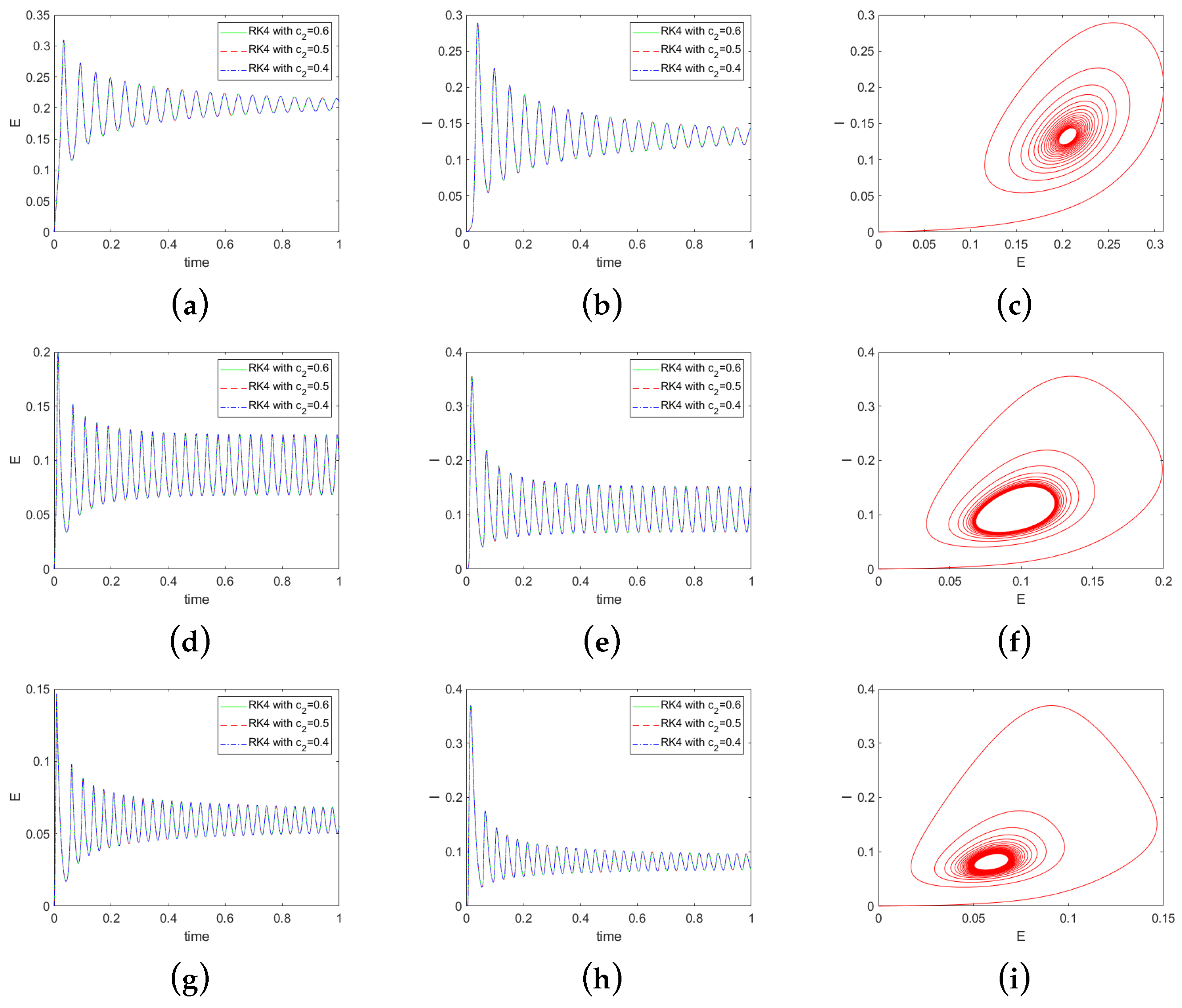
Figure 2.
Solutions for different matrix C using three fourth-order RK methods with , , and . First row (a–c): ; second row (d–f): ; third row (g–i): . Left column: the excitatory neural population; middle column: the inhibitory neural population; right column: the phase plane plot.
Figure 2.
Solutions for different matrix C using three fourth-order RK methods with , , and . First row (a–c): ; second row (d–f): ; third row (g–i): . Left column: the excitatory neural population; middle column: the inhibitory neural population; right column: the phase plane plot.
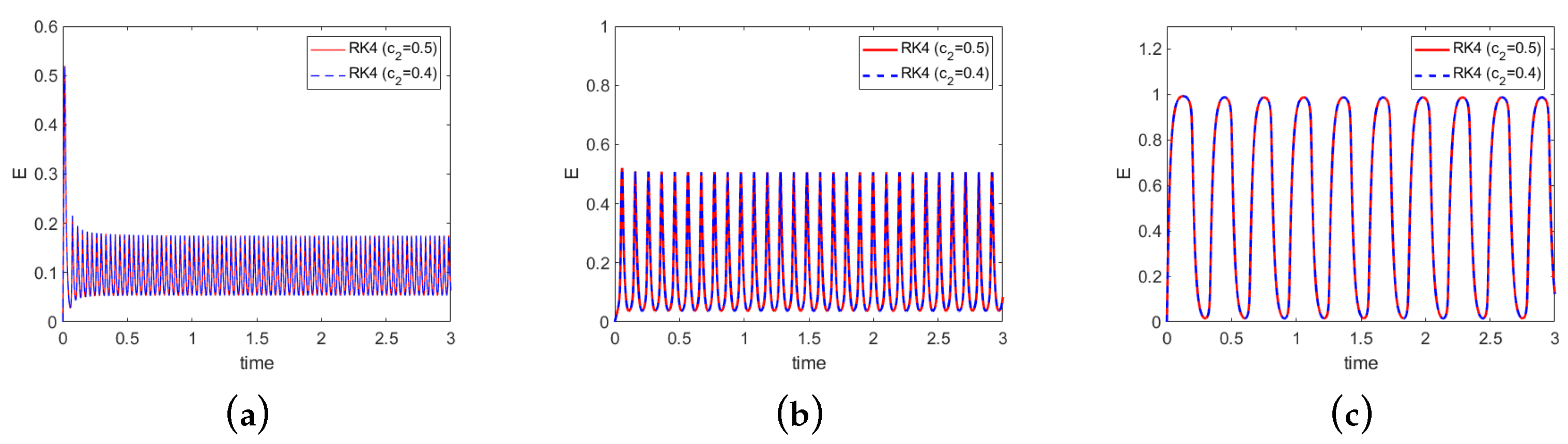
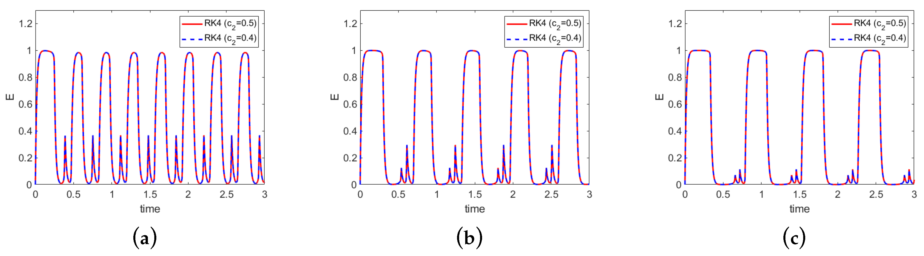
Figure 3.
Excitatory populations for single-spike waves: (a) T01, (b) T02, and (c) T03. Results of RK4-04 () and RK4-05 () are plotted in blue and red, respectively.
Figure 3.
Excitatory populations for single-spike waves: (a) T01, (b) T02, and (c) T03. Results of RK4-04 () and RK4-05 () are plotted in blue and red, respectively.
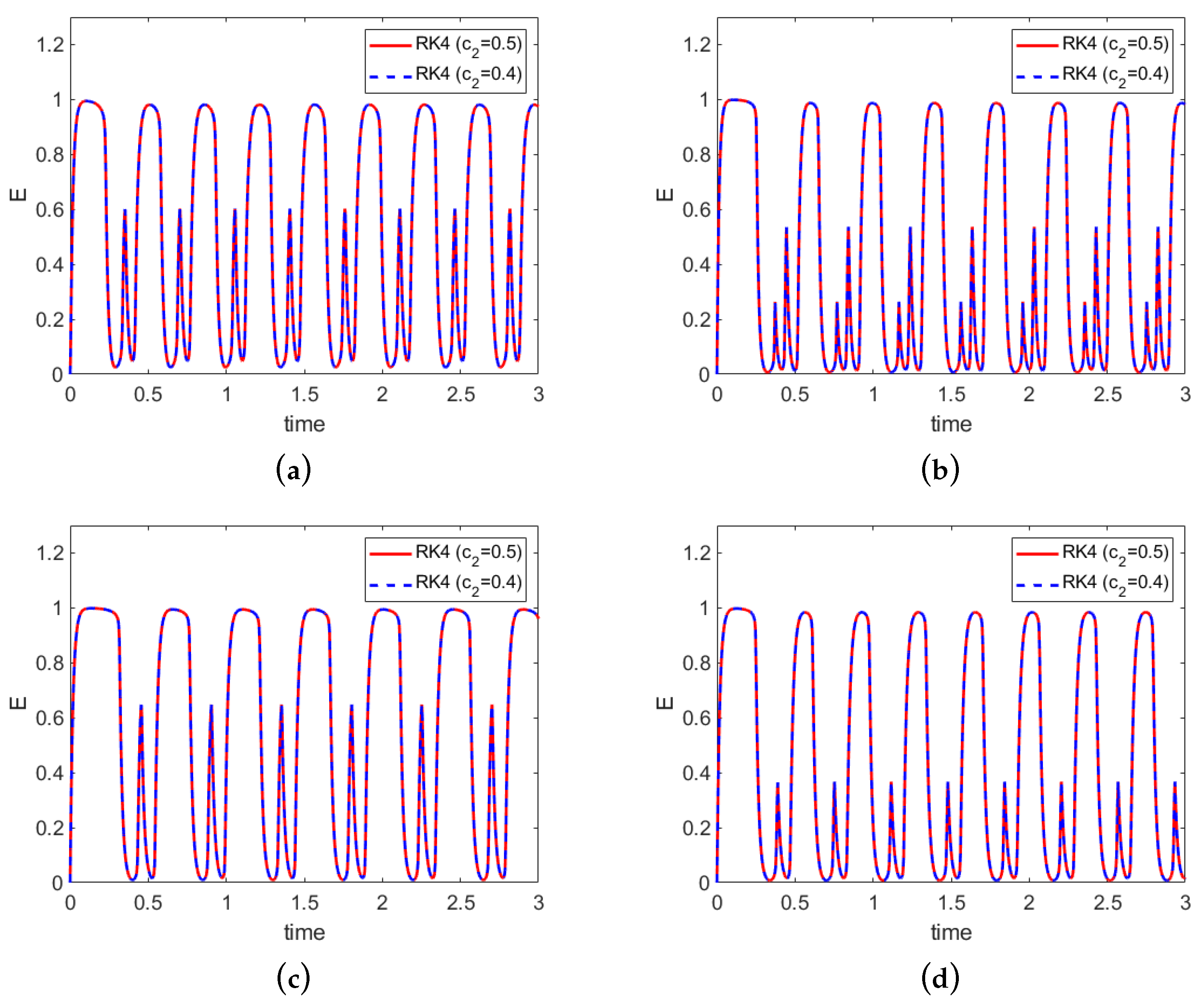
Figure 4.
Excitatory populations for poly-spike waves: (a) T04, (b) T05, (c) T06, and (b) T07. Results of RK4-04 () and RK4-05 () are plotted in blue and red, respectively.
Figure 4.
Excitatory populations for poly-spike waves: (a) T04, (b) T05, (c) T06, and (b) T07. Results of RK4-04 () and RK4-05 () are plotted in blue and red, respectively.
Figure 5.
Excitatory populations for test T04 with connection matrix , where (a) , (b) , and (c) . Results of RK4-04 () and RK4-05 () are plotted in blue and red, respectively.
Figure 5.
Excitatory populations for test T04 with connection matrix , where (a) , (b) , and (c) . Results of RK4-04 () and RK4-05 () are plotted in blue and red, respectively.
Figure 6.
Excitatory populations of test T07 with connection matrix , where (a) , (b) , and (c) . Results of RK4-04 () and RK4-05 () are plotted in blue and red, respectively.
Figure 6.
Excitatory populations of test T07 with connection matrix , where (a) , (b) , and (c) . Results of RK4-04 () and RK4-05 () are plotted in blue and red, respectively.
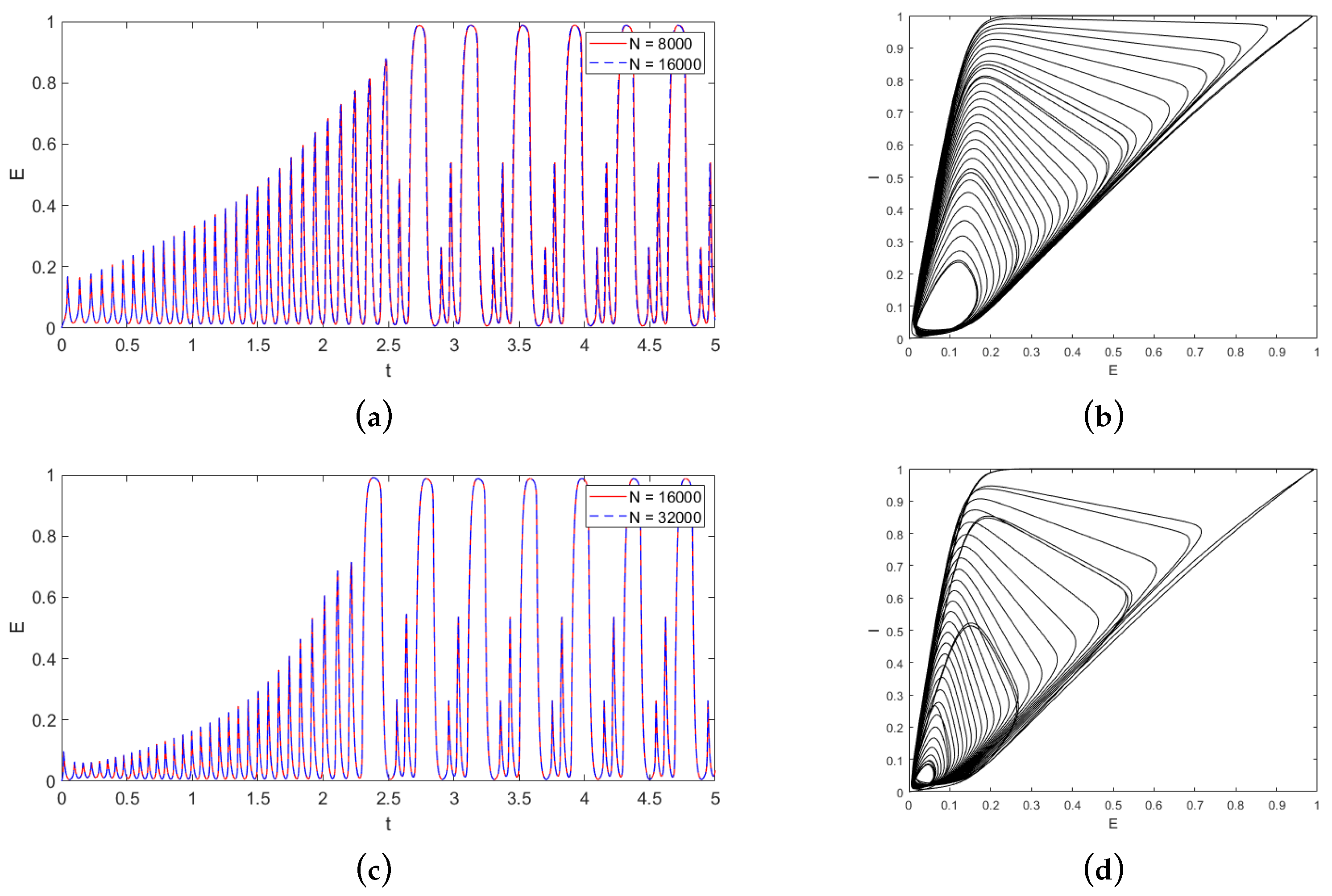
Figure 7.
Excitatory populations and the phase plane plots for test T05 with P gradually increases from 0 to 5. The connection matrix is . Upper row (a,b): is fixed at 1; lower row (c,d): gradually decreases from 2 to 1. Left column (a,c): excitatory neuron populations. Results of two resolutions N = 16,000 and N = 32,000 are plotted in red and blue, respectively. Right column (b,d): phase plane plots.
Table 1.
Coefficients for fourth-order RK methods when and varies from 0.1 to 0.9.
Table 1.
Coefficients for fourth-order RK methods when and varies from 0.1 to 0.9.
| Method | | | | | | | | | |
|---|
| RK4-01 | | | 1 | | | | | | |
| RK4-02 | | | 1 | | | | | | |
| RK4-03 | | | 1 | | | | | | |
| RK4-04 | | | 1 | | | | | | |
| RK4-05 | | | 1 | 1 | 1 | | | | |
| RK4-06 | | | 1 | | | | | | |
| RK4-07 | | | 1 | | | | | | |
| RK4-08 | | | 1 | | | | | | |
| RK4-09 | | | 1 | | | | | | |
Table 2.
Comparison of fourth-order RK methods when varies from 0.3 to 0.6. , and represent the numerical errors measured in the , , and norms, respectively.
Table 2.
Comparison of fourth-order RK methods when varies from 0.3 to 0.6. , and represent the numerical errors measured in the , , and norms, respectively.
| Method | N | | Rate | | Rate | | Rate |
|---|
| | 1000 | 7.96 × | | 2.98 × | | 2.12 × | |
| RK4-06 | 2000 | 4.60 × | 4.11 | 1.21 × | 4.62 | 1.17 × | 4.18 |
| 4000 | 2.61 × | 4.14 | 4.87 × | 4.64 | 6.50 × | 4.16 |
| | 8000 | 1.53 × | 4.10 | 2.01 × | 4.60 | 3.76 × | 4.11 |
| | 1000 | 7.90 × | | 3.01 × | | 2.29 × | |
| RK4-05 | 2000 | 4.57 × | 4.11 | 1.22 × | 4.63 | 1.26 × | 4.18 |
| 4000 | 2.63 × | 4.12 | 4.94 × | 4.62 | 7.10 × | 4.15 |
| | 8000 | 1.55 × | 4.08 | 2.06 × | 4.59 | 4.14 × | 4.10 |
| | 1000 | 2.29 × | | 9.33 × | | 8.38 × | |
| RK4-04 | 2000 | 1.32 × | 4.11 | 3.67 × | 4.67 | 4.31 × | 4.28 |
| 4000 | 7.10 × | 4.22 | 1.38 × | 4.74 | 2.20 × | 4.29 |
| | 8000 | 3.94 × | 4.17 | 5.37 × | 4.68 | 1.19 × | 4.21 |
| | 1000 | 3.79 × | | 1.55 × | | 1.36 × | |
| RK4-03 | 2000 | 2.68 × | 3.82 | 7.49 × | 4.38 | 8.70 × | 3.97 |
| 4000 | 1.70 × | 3.98 | 3.31 × | 4.50 | 5.34 × | 4.03 |
| | 8000 | 1.05 × | 4.02 | 1.44 × | 4.52 | 3.27 × | 4.03 |
Table 3.
Comparison of nine fourth-order RK methods when varies from 0.1 to 0.9. . , and represent the numerical errors measured in the , , and norms, respectively.
Table 3.
Comparison of nine fourth-order RK methods when varies from 0.1 to 0.9. . , and represent the numerical errors measured in the , , and norms, respectively.
| Method | | | | |
|---|
| RK4-01 | 0.1 | 1.11 × | 1.86 × | 8.91 × |
| RK4-02 | 0.2 | 1.47 × | 2.18 × | 5.91 × |
| RK4-03 | 0.3 | 1.05 × | 1.44 × | 3.27 × |
| RK4-04 | 0.4 | 3.94 × | 5.37 × | 1.19 × |
| RK4-05 | 0.5 | 1.55 × | 2.06 × | 4.14 × |
| RK4-06 | 0.6 | 1.53 × | 2.01 × | 3.76 × |
| RK4-07 | 0.7 | 2.70 × | 3.86 × | 9.30 × |
| RK4-08 | 0.8 | 1.25 × | 1.70 × | 3.71 × |
| RK4-09 | 0.9 | 5.37 × | 7.19 × | 1.50 × |
Table 4.
Comparison of errors for fourth-order RK methods with different values when varies from 0.1 to 5. The corresponding spectral radius varies from 3 to 146. .
Table 4.
Comparison of errors for fourth-order RK methods with different values when varies from 0.1 to 5. The corresponding spectral radius varies from 3 to 146. .
| | | | | | |
|---|
| 0.1 | 3 | 2.62 × | 2.03 × | 2.06 × | 2.03 × | 1.78 × |
| 0.5 | 15 | 2.36 × | 6.25 × | 3.82 × | 3.94 × | 1.52 × |
| 1 | 29 | 3.09 × | 1.41 × | 4.18 × | 3.85 × | 8.40 × |
| 1.5 | 44 | 3.36 × | 2.81 × | 8.98 × | 1.04 × | 6.42 × |
| 2 | 58 | 1.72 × | 4.97 × | 1.39 × | 1.90 × | 2.31 × |
| 5 | 146 | 2.70 × | 1.90 × | 4.58 × | 7.05 × | 1.41 × |
Table 5.
Comparison of errors for fourth-order RK methods with different values, as varies from 0.1 to 5. .
Table 5.
Comparison of errors for fourth-order RK methods with different values, as varies from 0.1 to 5. .
| | | | | | |
|---|
| 0.1 | 28 | 2.59 × | 4.40 × | 3.98 × | 4.18 × | 1.19 × |
| 0.5 | 29 | 4.88 × | 8.17 × | 8.48 × | 7.43 × | 1.61 × |
| 1 | 29 | 3.09 × | 1.41 × | 4.18 × | 3.85 × | 8.40 × |
| 1.5 | 30 | 4.08 × | 5.34 × | 2.45 × | 1.27 × | 3.35 × |
| 2 | 30 | 1.95 × | 1.61 × | 9.07 × | 5.58 × | 6.21 × |
| 5 | 113 | 7.08 × | 2.86 × | 1.83 × | 1.45 × | 2.33 × |
Table 6.
Comparison of errors for for fourth-order RK methods with different values, as varies from 0.1 to 5. .
Table 6.
Comparison of errors for for fourth-order RK methods with different values, as varies from 0.1 to 5. .
| | | | | | |
|---|
| 0.1 | 19 | 1.90 × | 1.04 × | 5.83 × | 3.28 × | 3.33 × |
| 0.5 | 21 | 4.26 × | 3.94 × | 1.76 × | 4.79 × | 2.04 × |
| 1 | 29 | 3.09 × | 1.41 × | 4.18 × | 3.85 × | 8.40 × |
| 1.5 | 35 | 3.45 × | 1.02 × | 3.71 × | 3.11 × | 1.07 × |
| 2 | 41 | 1.23 × | 5.39 × | 1.23 × | 8.81 × | 4.12 × |
| 5 | 64 | 7.78 × | 4.82 × | 6.23 × | 3.54 × | 2.73 × |
Table 7.
Comparison of errors for fourth-order RK methods with different values, as varies from 0.1 to 5. .
Table 7.
Comparison of errors for fourth-order RK methods with different values, as varies from 0.1 to 5. .
| | | | | | |
|---|
| 0.1 | 19 | 2.17 × | 1.48 × | 8.61 × | 5.35 × | 5.68 × |
| 0.5 | 21 | 5.98 × | 7.38 × | 1.59 × | 1.21 × | 2.41 × |
| 1 | 29 | 3.09 × | 1.41 × | 4.18 × | 3.85 × | 8.40 × |
| 1.5 | 35 | 6.25 × | 3.08 × | 2.54 × | 1.39 × | 2.61 × |
| 2 | 41 | 1.91 × | 1.98 × | 1.35 × | 1.23 × | 8.85 × |
| 5 | 64 | 1.26 × | 2.70 × | 1.87 × | 1.87 × | 7.33 × |
Table 8.
Comparison of errors for fourth-order RK methods with different values, as varies from 0.1 to 5. .
Table 8.
Comparison of errors for fourth-order RK methods with different values, as varies from 0.1 to 5. .
| | | | | | |
|---|
| 0.1 | 28.4 | 1.57 × | 6.10 × | 2.23 × | 2.17 × | 4.20 × |
| 0.5 | 28.7 | 2.17 × | 9.43 × | 3.03 × | 2.86 × | 5.84 × |
| 1 | 29.1 | 3.09 × | 1.41 × | 4.18 × | 3.85 × | 8.40 × |
| 1.5 | 29.5 | 4.18 × | 1.88 × | 5.47 × | 4.96 × | 1.16 × |
| 2 | 29.9 | 5.50 × | 2.34 × | 6.93 × | 6.18 × | 1.55 × |
| 5 | 32.2 | 2.60 × | 1.92 × | 2.06 × | 2.89 × | 1.92 × |
Table 9.
Parameters for the Wilson–Cowan model for epileptic dynamic simulations [
7].
Table 9.
Parameters for the Wilson–Cowan model for epileptic dynamic simulations [
7].
| Test | Figure in [7] | | | C |
|---|
| T01 | 3c | | | |
| T02 | 3f | | | |
| T03 | 3i | | | |
| T04 | 3l | | | |
| T05 | 4 | | | |
| T06 | 5d | | | |
| T07 | 5e | | | |
| T08 | 7 | | (−0.5, −5, 0) | |
Table 10.
errors of fourth-order RK methods with different values for tests T01 through T07.
Table 10.
errors of fourth-order RK methods with different values for tests T01 through T07.
| Test | T01 | T02 | T03 | T04 | T05 | T06 | T07 |
|---|
| 1.17 × | 5.78 × | 2.23 × | 1.61 × | 4.56 × | 4.36 × | 6.62 × |
| 5.81 × | 7.87 × | 1.52 × | 1.84 × | 4.89 × | 5.58 × | 6.04 × |
| 1.80 × | 4.22 × | 8.10 × | 8.97 × | 4.05 × | 4.13 × | 5.26 × |
| 1.77 × | 6.14 × | 4.48 × | 1.44 × | 6.40 × | 6.14 × | 8.83 × |
Table 11.
errors of fourth-order RK methods for test T04 with connection matrix , where varies from 1 to 3.
Table 11.
errors of fourth-order RK methods for test T04 with connection matrix , where varies from 1 to 3.
| Method | | | |
|---|
| RK4-03 () | 1.61 × | 1.99 × | 3.15 × |
| RK4-04 () | 1.84 × | 2.46 × | 3.20 × |
| RK4-05 () | 8.97 × | 2.13 × | 3.99 × |
| RK4-06 () | 1.44 × | 3.19 × | 6.21 × |
Table 12.
errors of fourth-order RK methods for test T04 with coupling coefficient , where varies from 1 to 3.
Table 12.
errors of fourth-order RK methods for test T04 with coupling coefficient , where varies from 1 to 3.
| Method | | | |
|---|
| RK4-03 () | 1.61 × | 2.30 × | 6.84 × |
| RK4-04 () | 1.84 × | 5.45 × | 3.61 × |
| RK4-05 () | 8.97 × | 4.55 × | 5.63 × |
| RK4-06 () | 1.44 × | 1.91 × | 1.06 × |
Table 13.
errors of fourth-order RK methods for test T07 with connection matrix , where varies from 1 to 2.
Table 13.
errors of fourth-order RK methods for test T07 with connection matrix , where varies from 1 to 2.
| Method | | | |
|---|
| RK4-03 () | 6.62 × | 2.26 × | 2.19 × |
| RK4-04 () | 6.04 × | 2.57 × | 5.07 × |
| RK4-05 () | 5.26 × | 3.31 × | 9.02 × |
| RK4-06 () | 8.83 × | 5.02 × | 1.52 × |
Table 14.
errors of fourth-order RK methods for test T05, as P gradually increases from 0 to 5. is fixed at 1 or gradually decreases from 2 to 1.
Table 14.
errors of fourth-order RK methods for test T05, as P gradually increases from 0 to 5. is fixed at 1 or gradually decreases from 2 to 1.
| Method | | Decreases from 2 to 1 |
|---|
| RK4-03 () | 2.19 × | 1.82 × |
| RK4-04 () | 2.70 × | 1.89 × |
| RK4-05 () | 2.18 × | 3.06 × |
| RK4-06 () | 3.26 × | 4.65 × |


