Article

Radiomic-Based Machine Learning for Differentiating Brain Metastases Recurrence from Radiation Necrosis Post-Gamma Knife Radiosurgery: A Feasibility Study

by
Mateus Blasques Frade
1,
Paola Critelli
2,
Eleonora Trifiletti
3,
Giuseppe Ripepi
4 and
Antonio Pontoriero
5,*
1
Department of Biomedical, Dental Science and Morphological and Functional Images, University of Messina, 98125 Messina, Italy
2
Radiation Oncology Department, Santa Croce and Carle Hospital, 12100 Cuneo, Italy
3
Department of Biomedical Dental and Morphological and Functional Imaging (BIOMORF), Residency School of Radiation Oncology, University of Messina, Via Consolare Valeria 1, 98124 Messina, Italy
4
I.I.S. “N. Pizi”—Ministry of Education and Merit, 89015 Palmi, Italy
5
Radiation Oncology Unit, Department of Biomedical, Dental Science and Morphological and Functional Images, University of Messina, 98125 Messina, Italy
*
Author to whom correspondence should be addressed.
Int. J. Transl. Med. 2025, 5(4), 50; https://doi.org/10.3390/ijtm5040050
Submission received: 25 August 2025 / Revised: 17 October 2025 / Accepted: 19 October 2025 / Published: 24 October 2025

Abstract

Background: Radiation therapy is a key treatment modality for brain metastases. While providing a treatment alternative, post-treatment imaging often presents diagnostic challenges, particularly in distinguishing tumor recurrence from radiation-induced changes such as necrosis. Advanced imaging techniques and artificial intelligence (AI)-based radiomic analyses emerge as alternatives to help lesion characterization. The objective of this study was to assess the capacity of machine learning algorithms to distinguish between brain metastases recurrence and radiation necrosis. Methods: The research was conducted in two phases and used publicly available MRI data from patients treated with Gamma Knife radiosurgery. In the first phase, 30 cases of local recurrence of brain metastases and 30 cases of radiation-induced necrosis were considered. Image segmentation and radiomic feature extraction were performed on these data using MatRadiomics_1_5_3, a MATLAB-based framework integrating PyRadiomics. Features were then selected using point-biserial correlation. In the second phase, a classification was performed using a Support Vector Machine model with repeated stratified cross-validation settings. Results: The results achieved an accuracy on the test set of 83% for distinguishing metastases from necrosis. Conclusions: The results of this feasibility study demonstrate the potential of radiomics and AI to improve diagnostic accuracy and personalized care in neuro-oncology.

1. Introduction

1.1. Radiomics and Machine Learning

Brain metastases (BMs) are the most common type of cancer that affects the central nervous system (CNS); about 30–40% of cancer patients have them or are going to develop them through their disease progression [1,2]. They are a well-known sign of a bad prognosis, and without timely and appropriate clinical intervention, patient outcomes tend to be particularly poor, which emphasizes the need for quick diagnosis and the use of individualized, multidisciplinary management strategies [3,4]. Beyond the morbidity directly caused by the BM to the CNS, treatment-related side effects play a major role in overall patient morbidity.
Systemic therapies are known to have reduced intracranial efficacy, which makes radiation therapy (RT), mainly stereotactic radiosurgery (SRS), an important treatment option. SRS must be carefully managed to avoid potential adverse effects. Radiation-induced toxicity can cause early (acute) and delayed (late) damage to nearby healthy tissues [5]. A critical challenge in the follow-up of post-radiotherapy BM patients is to differentiate between the BM lesions and radiation-induced changes, like radiation necrosis (RN). High-resolution imaging is necessary for the RT workflow to precisely define target volumes and identify organs at risk (OARs). To differentiate BM from perilesional edema and normal brain superior structures, magnetic resonance imaging (MRI) is often used for soft tissue contrast.
Radiomics is a way to translate information from medical images to numbers. The idea is that medical imaging contains information that is not readily visible but can be decoded using mathematical models. It allows a better thorough examination of tumor heterogeneity and treatment response, while conventional imaging is observer-dependent, and when it comes to difficult clinical scenarios, a misdiagnosis can happen [6]. Machine learning models that incorporate radiomics features have been shown to be effective in distinguishing between patients who will respond positively to RT and patients who will not [7]. Moreover, when trained on multiparametric MRI (including diffusion-weighted and perfusion imaging), machine learning algorithms have shown a high capability to differentiate radiation-induced necrosis from tumor recurrence [8].
The ability of AI-enhanced techniques, particularly quantitative radiomic features and Support Vector Machine algorithms, to differentiate between radiation-induced necrosis and brain metastases recurrence on post-radiotherapy MRI scans is assessed in this work. The main hypothesis is that quantitative radiomic signatures can be used to train machine learning algorithms to replicate the results of specialists and support this complex diagnostic differentiation. The development of such modelsserves as an aid for clinical workflow decision-support, to assist radiation oncologists in evaluating imaging data, and to improve post-treatment monitoring.

1.2. Support Vector Machine

Support Vector Machine (SVM) is a supervised learning model used for classification and regression tasks. It optimizes generalization ability, that is, the ability to recognize patterns that do not belong to the training set.
For the following notation, please refer to Appendix A. Let us now consider the training set T = {xi, yi}, i = 1, …, n, as the set of samples xi with relative labels yi identifying their class. Let us also consider a hyperplane separating classes:
w Φ x + b = 0
where w is the normal vector, b represents the bias term, and Φ is a transformation that allows the classification into the feature space, that is, a space of higher dimension than the sample space, where the decision boundary becomes linear (Figure 1).
Therefore, learning to classify these samples consists of computing the best decision hyperplane, that is, the one that maximizes the distance between the hyperplane itself and the nearest data points (i.e., samples in the feature space) from both classes. This distance is called the margin, and the nearest data points are support vectors. It requires the solution of the following optimization problem [9]:
m i n w , b , { ξ i } 1 2 w 2 + C i = 1 n ξ i
subject to the constraints:
y i w Φ x i + b 1 ξ i , ξ i 0 , i = 1 , , n
where y1, y2, …,yn are the labels of all patterns, C > 0 is the regularization parameter controlling the trade-off between margin size and classification error, and ξ1, ξ2, …, ξn are the so-called slack variablesthat allow for outlier tolerance so that the margin is not affected, and measure how much these points violate the margin or the decision boundary (Figure 2).
The problem of learning in an SVM can also be written in the dual form
m a x 1 T α 1 2 α T Q α
y T α = 0
0 α i C , i = 1 , , n
where 1 = (1, …,1) is the n-dimensional all-ones vector, Q is the matrix of coefficients, y = (y1, …, yn) are the above labels, and α = (α1, …, αn) are the Lagrange multipliers, i.e., auxiliary variables associated with the constraints of the problem which play the role of dual variables. The dual form makes it unnecessary to explicitly represent the transformation Φ. The elements of Q are then calculated as follows:
q i j = y i y j K x i , x j
where K is called the kernel function and implements the transformation Φ.
Thus, training an SVM means solving a convex quadratic programming problem with linear constraints, finding the optimal decision surface that allows the two classes to be discriminated.

2. Materials and Methods

2.1. Software and Tools Used

Image processing and feature extraction tasks were performed using MATLAB R2021b [10], a software environment designed for engineering and scientific tasks, offering tools for data analysis, image and signal processing, control system design, wireless communication, and robotics applications. MATLAB includes a programming language, interactive apps, highly specialized libraries, and tools for automatically generating embedded code. MatRadiomics_1_5_3 was the plugin used in our work; its function is to facilitate the entire radiomics work. The platform allows users to start a new radiomics study or import an existing one, load and view DICOM (Digital Imaging and Communications in Medicine) images and related metadata, segment the ROI, upload external segmentations, extract features using PyRadiomics, select features using a new hybrid method that combines descriptive and inferential techniques, and apply machine learning models for analysis [11]. PyRadiomics, a Python library v3.12.8 [12] integrated within MATLAB, was used for standardized radiomic feature extraction. Manual segmentations were carried out entirely in MATLAB.

2.2. Data Sources and Preparation

Although the Brain-TR-GammaKnife dataset includes lesion-level annotations reviewed independently by two neuroradiologists and one radiation oncologist, it does not provide histopathological confirmation for each case. Therefore, the ground truth labels used in this study reflect expert consensus based on imaging and clinical follow-up rather than biopsy-proven diagnoses. This limitation is common in radiomic studies and must be considered when interpreting the model’s performance. The dataset used in this work is the Brain-TR-GammaKnife dataset, published by [13] and hosted by The Cancer Imaging Archive (TCIA). This publicly available dataset contains brain MRI scans and corresponding Gamma Knife stereotactic radiosurgery treatment planning data from 47 patients diagnosed with brain metastases. Each patient underwent T1-weighted MPRAGE MRI scans using a 1.5T Siemens Magnetom scanner with gadolinium contrast and 1 × 1 × 1 mm voxel resolution.
The dataset has been preprocessed to support lesion-level AI-based classification. Each patient’s datawas used once as a test set. Dose images were resampled to match the spatial resolution of the planning MRI scans. Lesion-level cropping was performed using annotated masks. Segmentation masks, dose maps, and clinical outcome labels were provided in the DICOM-RT format. The datasetwas fully anonymized and curated for AI-based radiotherapy studies. The dataset was imported as is after independent evaluation of lesions by two different neuroradiologists and an RO; no discrepancies were found.

2.3. Radiomic Feature Extraction and Analysis

2.3.1. Segmentation of ROI

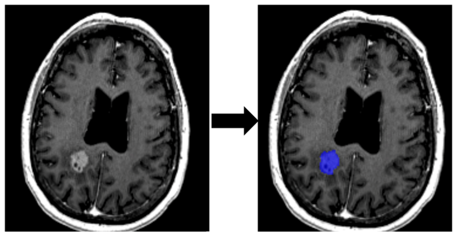
Lesions were manually segmented (Figure 3) using MatRadiomics_1_5_3, a MATLAB-based radiomics platform that supports feature extraction, selection, and predictive modeling.
Segmentation of lesions was performed under the supervision of a radiation oncologist with more than 10 years of clinical experience.

2.3.2. Feature Extraction

A total of 106 quantitative features were extracted using the PyRadiomics engine integrated into MATLAB. These features describe tumor morphology, signal intensity, and intra-lesional texture (Table 1).

2.3.3. Preprocessing and Training

The dataset was preprocessed in the following way. First, the 60 patterns were randomly divided into a training set (80% of the total, i.e., 48 patterns) and a test set (20%, 12 patterns). The training patterns were then subjected to scaling, i.e., their mean was scaled to 0 and variance to 1, applying the following criterion:
x = x μ σ
where x is an input pattern, µ and σ are, respectively, the mean and variance of the values of the training set, and x’ is the transformed (standardized) pattern. It is important to reiterate that mean and variance were calculated only on the training set to avoid data leakage, that is, to prevent test data from entering the training process and distorting the outcomes. Therefore, always only on the training set, the dimension of pattern space was reduced by Principal Component Analysis (PCA).
The training was performed by stratified k-fold cross-validation. In other words, the training set was divided into k partitions (folds), only one of which, in rotation, was used to measure the average performance of the model (Figure 4). On the other hand, stratification ensures that each fold preserves the original class distribution, which is particularly important for imbalanced datasets.
This pipeline (scaling + PCA + training) was then repeated n times with different random partitions of the data. By averaging results across several repetitions, this method reduces variance in the performance estimate and provides a more reliable assessment of model generalization. The values taken by k are 3, 4, 6, 8, and 12 in order to have balanced partitions, with n = 60.
To avoid information leakage, point-biserial correlation feature selection was performed within each training fold during the repeated stratified k-fold cross-validation. Specifically, for each fold, feature selection was applied only to the training subset, and the selected features were then used to train the model and evaluate it on the corresponding validation subset. This nested approach ensures that no information from the validation data influences the feature selection process.

2.3.4. Model Selection

In order to find the best model, the training was performed varying several parameters such as (1) number of PCA components by data variance; (2) regularization parameter C; (3) kernel function and (4) degree if it is polynomial; (5) kernel coefficient γ. The values of these parameters are shown and explained in Table 2.
The parameter n_components of the PCA was explored using four different settings: 0.90, 0.95, 0.99, and None. For instance, n_components = 0.90 retains the minimum number of principal components required to explain at least 90% of the variance, while n_components = 0.95 and n_components = 0.99 retain the number of components needed to explain 95% and 99% of the variance, respectively. This approach allows the dimensionality reduction to adapt automatically to the intrinsic structure of the dataset. Conversely, setting n_components = None means that no dimensionality reduction is applied: all components are retained, and the transformation corresponds to a full orthogonal rotation of the feature space. This also serves as a baseline condition, enabling comparison with reduced-dimensionality configurations. The rationale behind testing the thresholds 0.90, 0.95, and 0.99 is to investigate the trade-off between information retention and dimensionality reduction. Lower thresholds (e.g., 0.90) yield a more compact representation, potentially reducing noise but at the risk of discarding informative variance. Higher thresholds (e.g., 0.99) preserve nearly all variance, offering a minimal reduction in dimensionality, while the intermediate threshold (0.95) is a practical balance between the two extremes.
Model selection, as preprocessing and training, was carried out using ad hoc Python code (Appendix B).

3. Results

To better approximate clinical deployment and reduce the risk of data leakage, a leave-one-patient-out cross-validation (LOPO-CV) was performed. In this approach, each patient’s data was used exclusively for testing in one iteration, ensuring that no information from the same patient was present in both training and test sets.
The LOPO-CV yielded the following performance metrics: accuracy of 0.74, sensitivity of 0.95, specificity of 0.59, positive predictive value (PPV) of 0.63, and negative predictive value (NPV) of 0.94. These results confirm the model’s ability to reliably identify true positive cases while maintaining acceptable performance in ruling out false negatives, which is particularly relevant in clinical decision-making.

3.1. Leave-One-Patient-Out Cross-Validation (LOPO-CV)

As mentioned above, the model was evaluated on an independent test set consisting of 12 cases, derived from a total dataset of 60 patterns, and using various metrics, as shown below. All training converges on the following results.
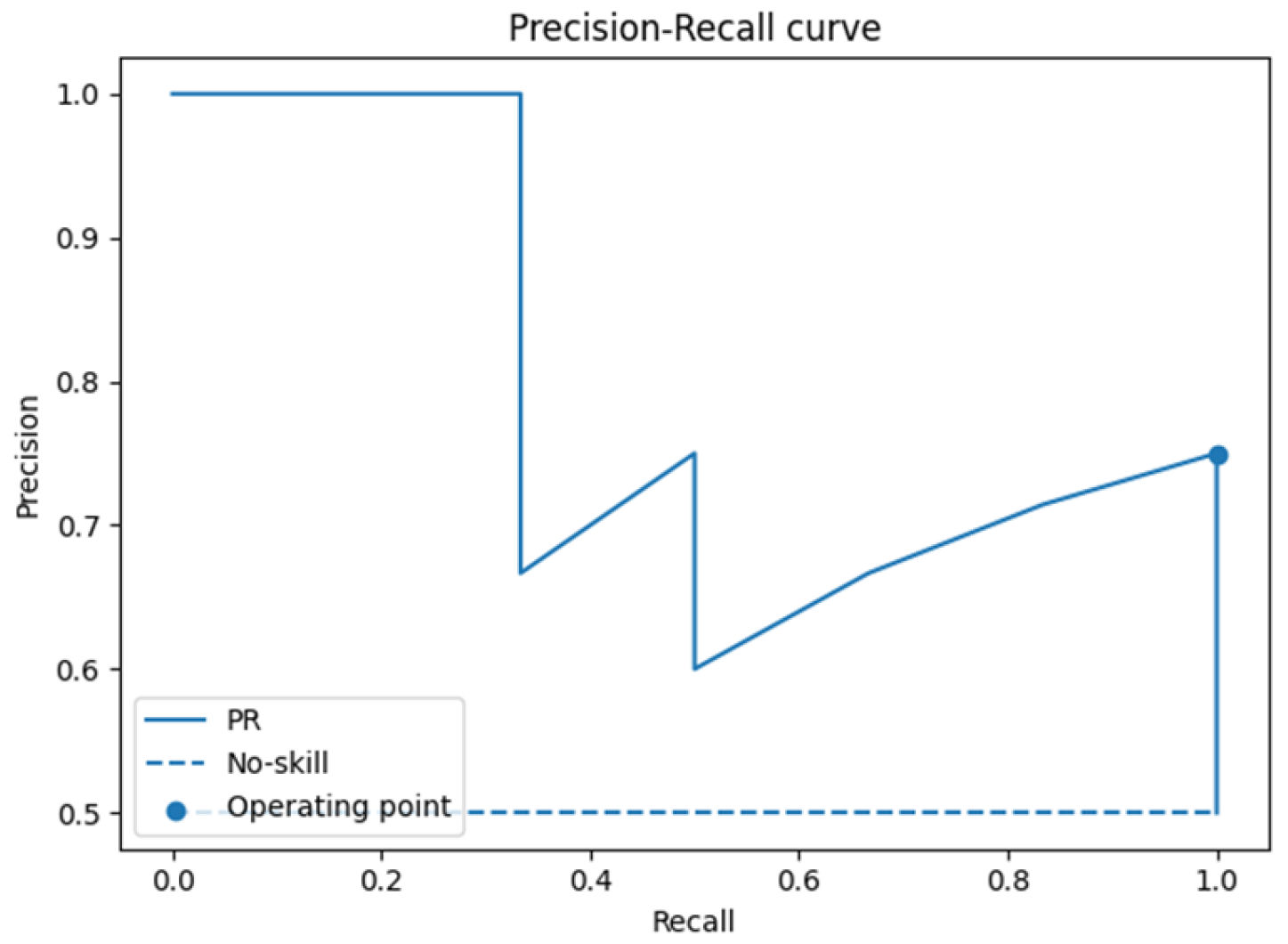
The ROC analysis (Figure 5) yielded an AUC of 0.80 (95% CI: 0.47–1.00), while the precision–recall analysis (Figure 6) showed an AUC of 0.83 (95% CI: 0.49–1.00). These values suggest acceptable discrimination. However, the wide confidence intervals, extending from values close to chance level to near-perfect classification, reflect the uncertainty arising from the limited test set size.
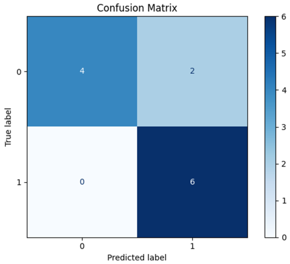
The confusion matrix (Figure 7) showed six true positives, four true negatives, two false positives, and no false negatives. Derived performance indices included an accuracy of 0.83, sensitivity of 1.00, specificity of 0.67, positive predictive value (PPV) of 0.75, and negative predictive value (NPV) of 1.00. These results indicate that the model successfully identified all positive cases, but at the expense of some false positive predictions.
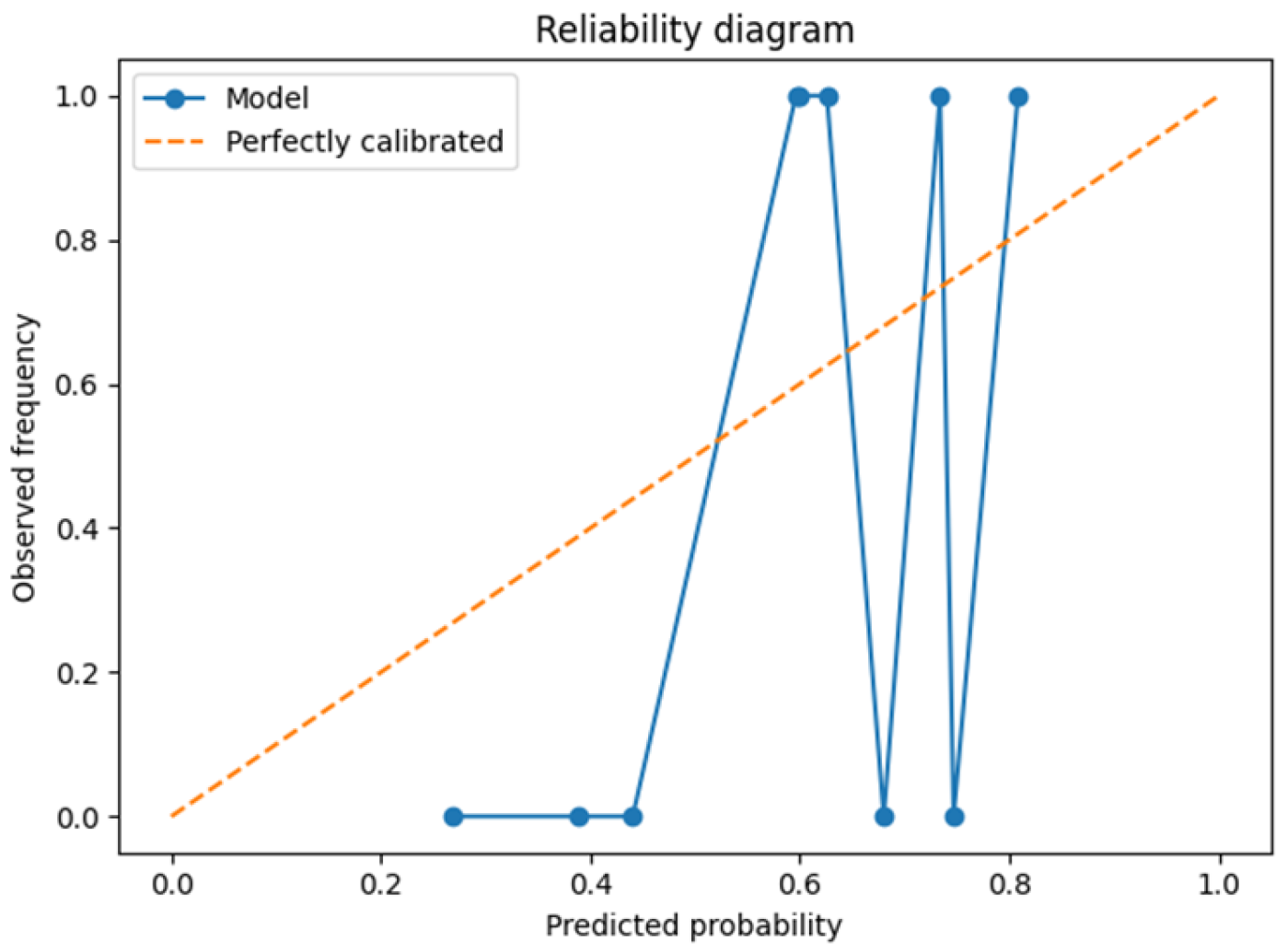
The reliability diagram (Figure 8) suggested that predicted probabilities were broadly aligned with observed frequencies. The Brier score of 0.18 confirmed moderate calibration, though this finding must be interpreted with caution due to the limited number of observations in the test set.
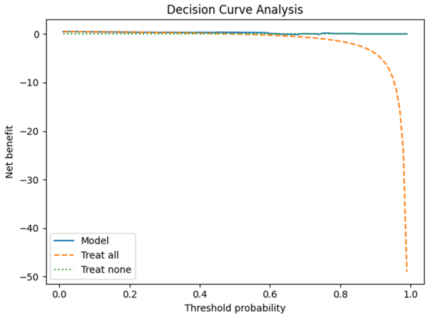
Finally, decision curve analysis (DCA, Figure 9) indicated that the model may provide a net clinical benefit across a range of threshold probabilities, further supporting its potential utility. Nevertheless, as with other analyses, the small test set limits the robustness of these conclusions.
Table 3 summarises the above, and Table 4 shows the best parameters found in model selection.

3.2. Radiomic Feature Interpretability and Clinical Relevance

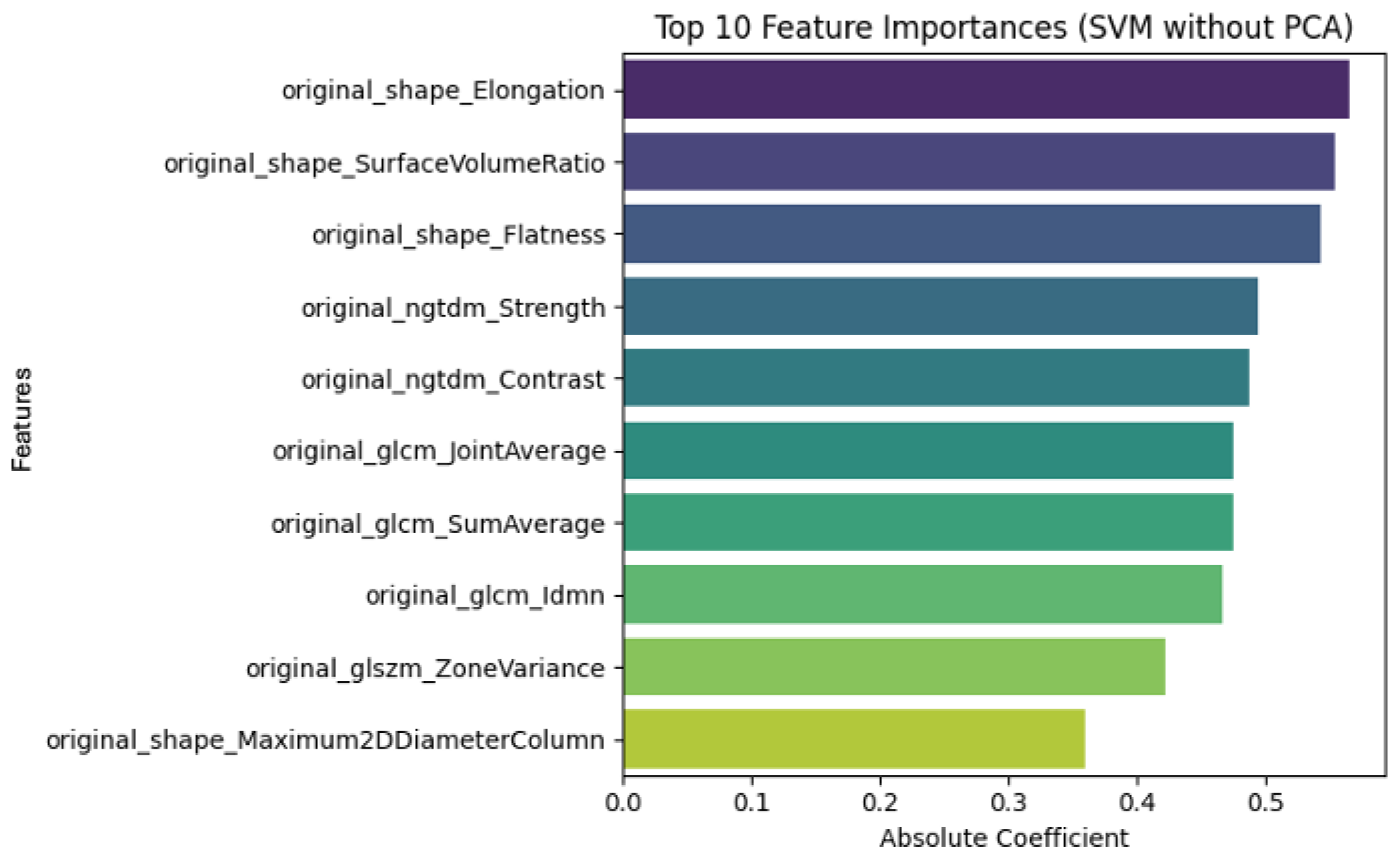
The linear SVM model trained without PCA (Figure 10) preserves the original radiomic features, allowing direct clinical interpretation. Among the most influential features in distinguishing tumor recurrence from radiation necrosis are texture descriptors (e.g., GLCM, and NGTDM) and shape-based metrics. These features are clinically meaningful: necrotic lesions typically present with irregular morphologies and heterogeneous signal patterns, while recurrent tumors tend to be more homogeneous and spherical.
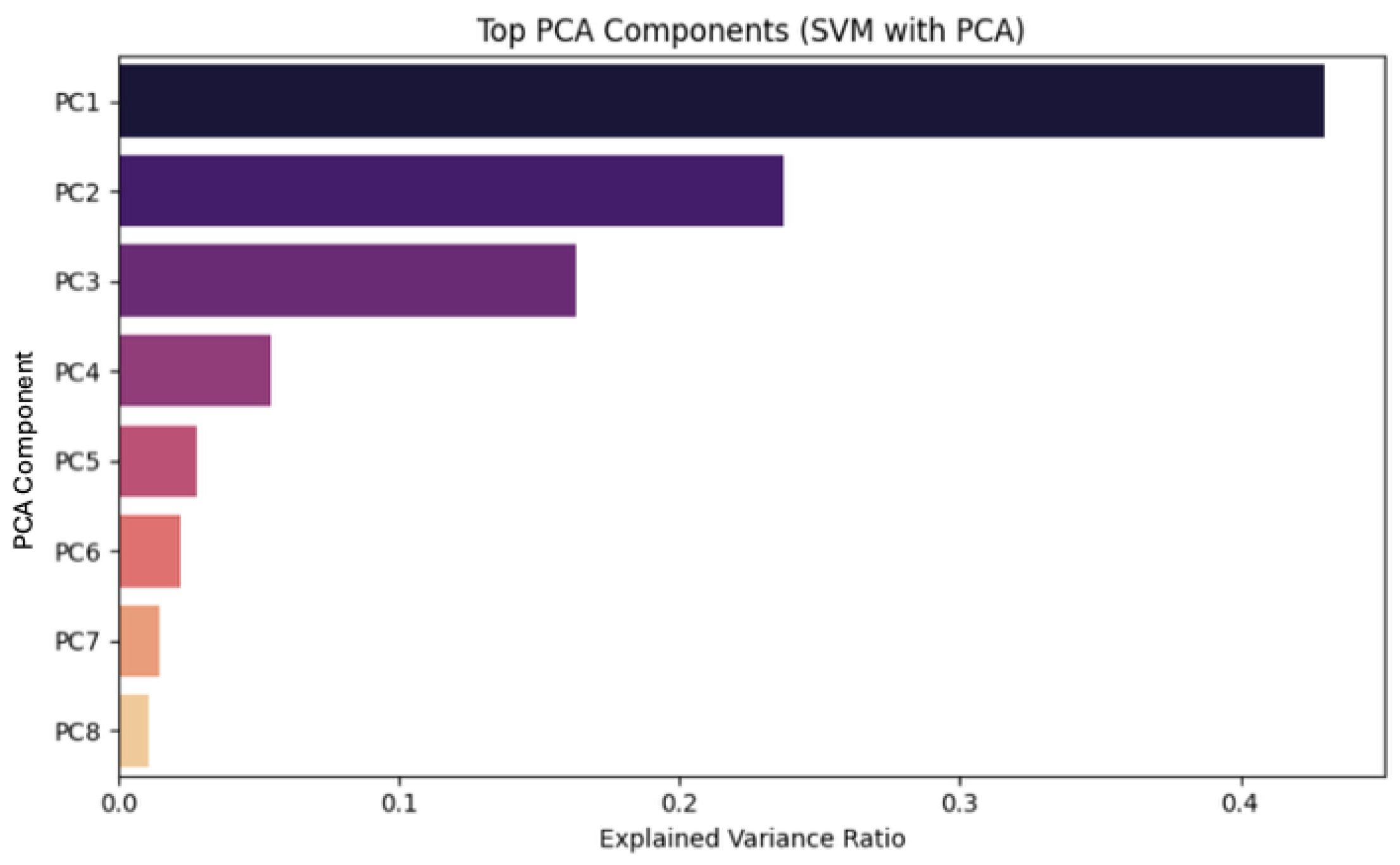
In contrast, when PCA (Figure 11) is applied, the model operates on transformed principal components rather than the original features. Although this approach reduces dimensionality and may enhance generalization, it limits direct interpretability. The top principal components capture most of the variance in the dataset, but their clinical meaning is less transparent.
To support interpretability, a SHAP-inspired analysis was performed, confirming that texture and shape features are key drivers in the classification task. These insights can assist clinicians in understanding the model’s decision-making process and facilitate the integration of radiomics into clinical workflows.
The SHAP analysis (Table 5) revealed that texture (e.g., difference entropy), shape (sphericity), and first-order (skewness) features were among the most influential in distinguishing radiation necrosis from tumor recurrence.

4. Discussion

This study should be considered a developmental investigation, given the limited sample size (n = 60 patterns from 47 patients). Its primary aim is to explore the feasibility of radiomic-based classification rather than to provide definitive clinical validation.
To better approximate clinical deployment and reduce overfitting risks, we implemented a leave-one-patient-out cross-validation (LOPO-CV) strategy. This approach ensures that each patient’s data is used exclusively for testing in one iteration, preventing any overlap between training and test sets. The LOPO-CV yielded promising results (accuracy = 0.74, sensitivity = 0.95, NPV = 0.94), particularly in minimizing false negatives, which is critical in clinical decision-making.
We acknowledge that external validation is essential for future work, and we plan to incorporate multicenter or time-split data from TCIA or other repositories to assess generalizability and robustness.
Regarding clinical thresholds, we performed decision curve analysis (DCA) to evaluate the net benefit across a range of operating points. This analysis supports the potential utility of the model in real-world settings, where rule-in and rule-out thresholds may vary depending on clinical context. For example, in a multidisciplinary tumor board, a high-sensitivity threshold might be preferred to rule out recurrence when biopsy is not feasible, whereas a high-specificity threshold could be used to confirm recurrence before initiating salvage therapy.

4.1. Dimensionality Reduction

After scaling, PCA was applied to the dataset as a preprocessing step before the SVM training. Several thresholds were tested (90%, 95%, 99%, and full retention) in order to determine the best performance, achieved by full retention of the components.
Another analysis conducted independently of the SVM training showed that a single principal component was sufficient to explain nearly all of the dataset’s variance, even under a stringent 99% retention threshold. This outcome confirms the presence of a dominant direction of variability, but a more detailed examination of this finding is provided in Appendix C.

4.2. SVM Classification and Model Robustness

The classification step involved SVMs with multiple kernel options and regularization strategies that were optimized by a thorough grid search and repeated stratified k-fold cross-validation. Linear kernels have consistently outperformed non-linear alternatives, which indicates that the decision boundary was approximately linear, supporting proper feature selection and transformationin simplifying the classification task, even in complex imaging data.
In fact, the model achieved excellent sensitivity (1.00) and NPV (1.00), suggesting that it may be particularly effective in contexts where avoiding false negatives is critical. In contrast, specificity (0.67) and PPV (0.75) were more modest, highlighting the occurrence of false positives. Furthermore, the performance metrics and graphical assessments (ROC, precision–recall, calibration, and DCA) provide a consistent picture of a model with encouraging preliminary characteristics. However, the statistical uncertainty is substantial, as reflected by the wide confidence intervals for most metrics. In a test set of only 12 cases, even a single misclassification exerts a large effect on sensitivity, specificity, and predictive values, thereby limiting the generalizability of these findings.
Finally, calibration analysis and the Brier score suggest that probability estimates are reasonably well calibrated, but these results are again constrained by the small denominator. Similarly, the decision curve analysis points to a potential net benefit, though such conclusions remain provisional given the exploratory nature of the study.

4.3. Limitations and Future Work

Another important limitation concerns the biological heterogeneity of the lesions. In clinical practice, it is not uncommon for a single lesion to contain both viable tumor cells and radiation-induced necrotic tissue. These ‘mixed lesions’ challenge binary classification models, as they do not represent purely recurrent or purely necrotic entities. Future work should explore probabilistic or multi-label approaches that can reflect the continuum of tissue composition and provide more nuanced diagnostic support.
This study should be regarded as an exploratory investigation aimed at assessing the feasibility of radiomic-based machine learning for the clinically relevant challenge of differentiating brain metastasis recurrence from radiation necrosis. While the sample size is limited (n = 60), our findings underscore the potential of this approach and highlight the need for external validation using larger, multicenter datasets to enable clinical translation and support timely, evidence-based decision-making.
The dataset used in this study does not include detailed information on systemic therapies, such as targeted agents and immunotherapies, which are increasingly employed in the management of brain metastases. These treatments can induce pseudoprogression, a phenomenon that may mimic both tumor recurrence and radiation necrosis in imaging. Because this factor was not accounted for in the original dataset, our model may have inadvertently included cases of pseudoprogression without distinction. Future research should incorporate longitudinal clinical data and treatment history to better address this diagnostic challenge. In addition, we acknowledge the absence of gold-standard diagnostic criteria in the original dataset. Although the Brain-TR-GammaKnife dataset is publicly available and its labels were reviewed by two neuroradiologists and a radiation oncologist, no formal adjudication process was applied. This limitation may have introduced uncertainty in lesion classification. To mitigate this, we implemented a leave-one-patient-out cross-validation (LOPO-CV) strategy and performed a SHAP-inspired feature analysis to enhance interpretability and robustness. Nonetheless, the lack of a definitive reference standard warrants caution when interpreting our findings, which should be considered exploratory.
This development study achieved promising results, though several limitations must be addressed. The sample size (n = 60) is not large enough to provide thorough generalizability of the results. Even though repeated stratified k-fold cross-validation and strict training/test splits were used to mitigate this problem, larger datasets would be required for a more reliable translation into clinical practice. Future directions may encompass the augmentation of the dataset with multicenter data to improve generalizability, the integration of multi-parametric imaging modalities (e.g., perfusion-weighted imaging, diffusion MRI), and the incorporation of automatic or semi-automatic segmentation techniques. A next step of the current study might be the use of a larger dataset and the application of alternative machine learning methodologies.
Radiomic features act as quantitative surrogates of lesion biology, offering reproducible metrics that can complement conventional imaging interpretation. For example, high difference entropy values—derived from GLCM texture analysis—capture intralesional heterogeneity, a hallmark of necrotic tissue architecture. Low sphericity values, on the other hand, reflect morphological irregularities often seen in post-radiation changes. Clinically, these descriptors provide observer-independent evidence that can improve diagnostic confidence in differentiating recurrence from radionecrosis (Figure 12). Their integration into machine learning models enables stratified risk assessment and supports multidisciplinary decision-making, particularly in cases where conventional imaging yields equivocal findings or when biopsy is not feasible.
In a clinical setting, building a predictive model able to distinguish between brain metastases recurrence and radiation necrosis would not act autonomously but as a decision support tool in a multidisciplinary tumor board. Thresholds (rule-in and rule-out) may be adjusted dynamically depending on patient history, radiologist confidence, or availability of follow-up diagnostics.

Author Contributions

Conceptualization, A.P. and G.R.; methodology, A.P.; software, G.R.; validation, A.P., G.R. and M.B.F.; formal analysis, G.R. and M.B.F.; investigation, P.C.; resources, E.T.; data curation, M.B.F. writing—original draft preparation, M.B.F. writing—review and editing, M.B.F., G.R. and A.P.; visualization, G.R.; supervision, G.R. and A.P. All authors have read and agreed to the published version of the manuscript.

Funding

This research received no external funding.

Institutional Review Board Statement

Ethical review and approval were waived for this study because the Brain-TR-GammaKnife dataset presented in the study were obtained from The Cancer Imaging Archive and are available on https://www.cancerimagingarchive.net/collection/brain-tr-gammaknife/ accessed on 24 August 2025 with the permission of Cancer Imaging Archive.

Informed Consent Statement

Not applicable.

Data Availability Statement

The original contributions presented in this study are included in the article material. Further inquiries can be directed to the corresponding authors.

Acknowledgments

The authors would like to thank Giovanni Pasini for kindly providing the MaRadiomics software and for his valuable support in its application. Giovanni Pasini (Department of Mechanical and Aerospace Engineering (DIMA), Sapienza University of Rome, Rome, Italy. Institute of Bioimaging and Complex Biological Systems—National Research Council (IBSBC—CNR), Cefalù, Italy).

Conflicts of Interest

The authors declare no conflicts of interest.

Abbreviations

The following abbreviations are used in this manuscript:
BMBrain Metastases
CNSCentral Nervous System
RTRadiation Therapy
SRSStereotactic Radiosurgery
OARsOrgans at Risk
MRIMagnetic Resonance Imaging
ROIRegion of Interest
PBCPoint-Biserial Correlation
CVCross-validation
AIArtificial Intelligence
SVMSupport Vector Machine
PCAPrincipal Component Analysis

Appendix A

The mathematical content of the present work was reduced to the minimum necessary to achieve a proper understanding of the parameters in model training and selection. However, it is useful to specify the notation used. Vectors are denoted bylower-case bold letters, such as x. A superscript T denotes the transpose of a vector. The notation (x1, …, xn) denotes a vector with n elements, so xi is the i-th element of a vector, but xi is the i-th vector in a set. Patterns, i.e., samples, i.e., points of the input or feature space, are represented as vectors.

Appendix B

The SVM was implemented in Python due to its cross-platform compatibility and because it is easy and fast to develop machine learning code. The Scikit-learn library was used for scaling, Principal Component Analysis, training, testing, and for hyperparameter optimization in model selection. The Pandas library was also used to read the dataset, which is in CSV format. The source code is shown below.
import numpy as np
import pandas as pd
import matplotlib.pyplot as plt
from sklearn.model_selection import (
   train_test_split, RepeatedStratifiedKFold, GridSearchCV
   )
from sklearn.pipeline import Pipeline
from sklearn.preprocessing import StandardScaler
from sklearn.decomposition import PCA
from sklearn.svm import SVC
from sklearn.metrics import (
accuracy_score, confusion_matrix, roc_auc_score, average_precision_score,
precision_recall_curve, roc_curve, brier_score_loss
)
from sklearn.calibration import calibration_curve
from sklearn.metrics import ConfusionMatrixDisplay
 
# =========================
# 1) DATA & SPLIT
# =========================
df = pd.read_csv(‘dataset.csv’)
X = df.iloc[:, :-1].values
y = df.iloc[:, -1].values
 
X_train, X_test, y_train, y_test = train_test_split(
X, y, test_size=0.2, stratify=y, random_state=42
)
 
# =========================
# 2) PIPELINE + GRID + CV
# =========================
base_pipeline = Pipeline([
(‘scaler’, StandardScaler()),
(‘pca’, PCA()),
(‘svm’, SVC(probability=True, random_state=42))
])
 
param_grid = {
‘pca__n_components’: [0.90, 0.95, 0.99, None],
‘svm__kernel’: [‘linear’, ‘rbf’, ‘poly’, ‘sigmoid’],
‘svm__C’: [0.1, 1, 10, 100],
‘svm__gamma’: [‘scale’, ‘auto’],
‘svm__degree’: [2, 3, 4]
}
 
nFolds = 6
nRepeats = 10
cv=RepeatedStratifiedKFold(n_splits=nFolds,n_repeats=nRepeats,random_state=42)
 
grid_search = GridSearchCV(
estimator=base_pipeline,
param_grid=param_grid,
scoring=‘accuracy’,
cv=cv,
n_jobs=-1,
verbose=0,
refit=True
)
 
grid_search.fit(X_train, y_train)
best_params = grid_search.best_params_
print(“Best parameters:“, best_params)
 
best_pipeline = Pipeline([
(‘scaler’, StandardScaler()),
(‘pca’, PCA(n_components=best_params[‘pca__n_components’])),
(‘svm’, SVC(
kernel=best_params[‘svm__kernel’],
C=best_params[‘svm__C’],
gamma=best_params[‘svm__gamma’],
degree=best_params.get(‘svm__degree’, 3),
probability=True,
random_state=42))
])
 
best_pipeline.fit(X_train, y_train)
 
# =========================
# 3) TEST
# =========================
y_pred = best_pipeline.predict(X_test)
y_proba = best_pipeline.predict_proba(X_test)[:, 1]
 
# =========================
# 4) CONFUSION MATRIX + METRICS
# =========================
cm = confusion_matrix(y_test, y_pred, labels=[0,1])
tn, fp, fn, tp = cm.ravel()
sens = tp/(tp + fn) if (tp + fn) > 0 else np.nan
spec = tn/(tn + fp) if (tn + fp) > 0 else np.nan
ppv = tp/(tp + fp) if (tp + fp) > 0 else np.nan
npv = tn/(tn + fn) if (tn + fn) > 0 else np.nan
acc = accuracy_score(y_test, y_pred)
 
disp = ConfusionMatrixDisplay(confusion_matrix=cm, display_labels=[0, 1])
disp.plot(cmap=“Blues”, values_format=“d”)
plt.title(“Confusion Matrix”)
plt.tight_layout()
plt.show()
 
# =========================
# 5) METRICS WITH 95% CI via BOOTSTRAP
# =========================
def bootstrap_metric(y_true,y_score, y_pred_labels, n_boot=2000, random_state=42):
rng = np.random.RandomState(random_state)
metrics = {
“roc_auc”: [], “pr_auc”: [], “brier”: [],
“sens”: [], “spec”: [], “ppv”: [], “npv”: [], “acc”: []
}
n = len(y_true)
 
for _ in range(n_boot):
idx = rng.randint(0, n, n) # campionamento con rimpiazzo
y_t = y_true[idx]
y_s = y_score[idx]
y_p = y_pred_labels[idx]
 
if len(np.unique(y_t)) < 2:
continue
 
try: metrics[“roc_auc”].append(roc_auc_score(y_t, y_s))
except: pass
try: metrics[“pr_auc”].append(average_precision_score(y_t, y_s))
except: pass
try: metrics[“brier”].append(brier_score_loss(y_t, y_s))
except: pass
 
cm_b = confusion_matrix(y_t, y_p, labels=[0,1])
if cm_b.size == 4:
tn_b, fp_b, fn_b, tp_b = cm_b.ravel()
metrics[“sens”].append(tp_b/(tp_b+fn_b) if (tp_b+fn_b) > 0 else np.nan)
metrics[“spec”].append(tn_b/(tn_b+fp_b) if (tn_b+fp_b) > 0 else np.nan)
metrics[“ppv”].append(tp_b/(tp_b+fp_b) if (tp_b+fp_b) > 0 else np.nan)
metrics[“npv”].append(tn_b/(tn_b+fn_b) if (tn_b+fn_b) > 0 else np.nan)
denom = tp_b + tn_b + fp_b + fn_b
metrics[“acc”].append((tp_b + tn_b)/denom if denom > 0 else np.nan)
 
def stats(values):
vals = np.array([v for v in values if not np.isnan(v)])
if len(vals) == 0:
return np.nan, np.nan, np.nan, np.nan
mean = np.mean(vals)
std = np.std(vals, ddof=1)
lo, hi = np.percentile(vals, 2.5), np.percentile(vals, 97.5)
return mean, std, lo, hi
 
results = {}
for k, v in metrics.items():
results[k] = stats(v)
return results
 
ci_results = bootstrap_metric(y_test,y_proba,y_pred, n_boot=2000, random_state=42)
 
def fmt_ci(name, point, std, lo, hi, decimals_pm=2, decimals_ci=4):
pm_str = f”{point:.{decimals_pm}f}”
err_str = f”{std:.{decimals_pm}f}” if np.isfinite(std) else “nan”
ci_str = f”{lo:.{decimals_ci}f}–{hi:.{decimals_ci}f}”
return f”{name}: {pm_str} ± {err_str} (95% CI {ci_str}, bootstrap)”
 
print(“\n--- Metrics with IC 95% (bootstrap on test) ---”)
print(fmt_ci(“ROC-AUC”, *ci_results[“roc_auc”]))
print(fmt_ci(“PR-AUC”, *ci_results[“pr_auc”]))
print(fmt_ci(“Brier”, *ci_results[“brier”]))
print(fmt_ci(“Sens”, *ci_results[“sens”]))
print(fmt_ci(“Spec”, *ci_results[“spec”]))
print(fmt_ci(“PPV”, *ci_results[“ppv”]))
print(fmt_ci(“NPV”, *ci_results[“npv”]))
print(fmt_ci(“Acc”, *ci_results[“acc”]))
 
# =========================
# 6) CURVE ROC & PR
# =========================
fpr, tpr, _ = roc_curve(y_test, y_proba)
prec, rec, _ = precision_recall_curve(y_test, y_proba)
 
plt.figure()
plt.plot(fpr, tpr, label=‘ROC’)
plt.plot([0,1], [0,1], linestyle=‘--‘, label=‘No-skill’)
plt.scatter([fp/(fp + tn)], [sens], label=‘Operating point’)
plt.xlabel(‘False Positive Rate’)
plt.ylabel(‘True Positive Rate’)
plt.title(‘ROC curve’)
plt.legend(loc=‘lower right’)
plt.tight_layout()
plt.show()
 
plt.figure()
plt.plot(rec, prec, label=‘PR’)
baseline = np.mean(y_test) # prevalenza
plt.hlines(baseline, 0, 1, linestyles=‘--‘, label=‘No-skill’)
plt.scatter([sens], [ppv], label=‘Operating point’)
plt.xlabel(‘Recall’)
plt.ylabel(‘Precision’)
plt.title(‘Precision-Recall curve’)
plt.legend(loc=‘lower left’)
plt.tight_layout()
plt.show()
 
# =========================
# 7) CALIBRATION: RELIABILITY DIAGRAM + BRIER
# =========================
brier = brier_score_loss(y_test, y_proba)
print(f”\nBrier score (single estimate): {brier:.4f}”)
 
prob_true,prob_pred=calibration_curve(
   y_test,y_proba,n_bins=10,strategy=‘quantile’
   )
plt.figure()
plt.plot(prob_pred, prob_true, marker=‘o’, label=‘Model’)
plt.plot([0,1], [0,1], linestyle=‘--‘, label=‘Perfectly calibrated’)
plt.xlabel(‘Predicted probability’)
plt.ylabel(‘Observed frequency’)
plt.title(‘Reliability diagram’)
plt.legend()
plt.tight_layout()
plt.show()
 
# =========================
# 8) DECISION CURVE ANALYSIS (Net Benefit)
# =========================
def decision_curve_net_benefit(y_true, y_prob, thresholds):
y_true = np.asarray(y_true)
y_prob = np.asarray(y_prob)
N = len(y_true)
prevalence = y_true.mean()
nb_model, nb_all, nb_none = [], [], []
 
for pt in thresholds:
y_pred = (y_prob >= pt).astype(int)
tn, fp, fn, tp = confusion_matrix(y_true, y_pred, labels=[0,1]).ravel()
w = pt/(1.0 - pt)
nb = (tp/N) - (fp/N) * w
nb_model.append(nb)
nb_all.append(prevalence - (1 - prevalence) * w)
nb_none.append(0.0)
 
return np.array(nb_model), np.array(nb_all), np.array(nb_none)
 
thresholds = np.linspace(0.01, 0.99, 99)
nb_model,nb_all,nb_none=decision_curve_net_benefit(y_test, y_proba, thresholds)
plt.figure()
plt.plot(thresholds, nb_model, label=‘Model’)
plt.plot(thresholds, nb_all, linestyle=‘--‘, label=‘Treat all’)
plt.plot(thresholds, nb_none, linestyle=‘:‘, label=‘Treat none’)
plt.xlabel(‘Threshold probability’)
plt.ylabel(‘Net benefit’)
plt.title(‘Decision Curve Analysis’)
plt.legend()
plt.tight_layout()
plt.show()

Appendix C

In order to investigate the dimensionality reduction outcome of PCA, we calculated the number of retained components required to explain a given proportion of the total variance in the dataset. Importantly, this evaluation was conducted independently of the subsequent SVM training, in order to isolate the intrinsic structure of the feature space (see source code in Appendix D). When applying a variance retention threshold of 99% (i.e., setting n_components = 0.99), the analysis consistently yielded a single principal component as sufficient to account for nearly the entire variability of the dataset. This finding reinforces the observation that the data exhibit a highly dominant direction of variance, whereby one component effectively captures the major patterns present across the features. Such a result suggests that the effective dimensionality of the problem is substantially lower than the raw number of input variables.
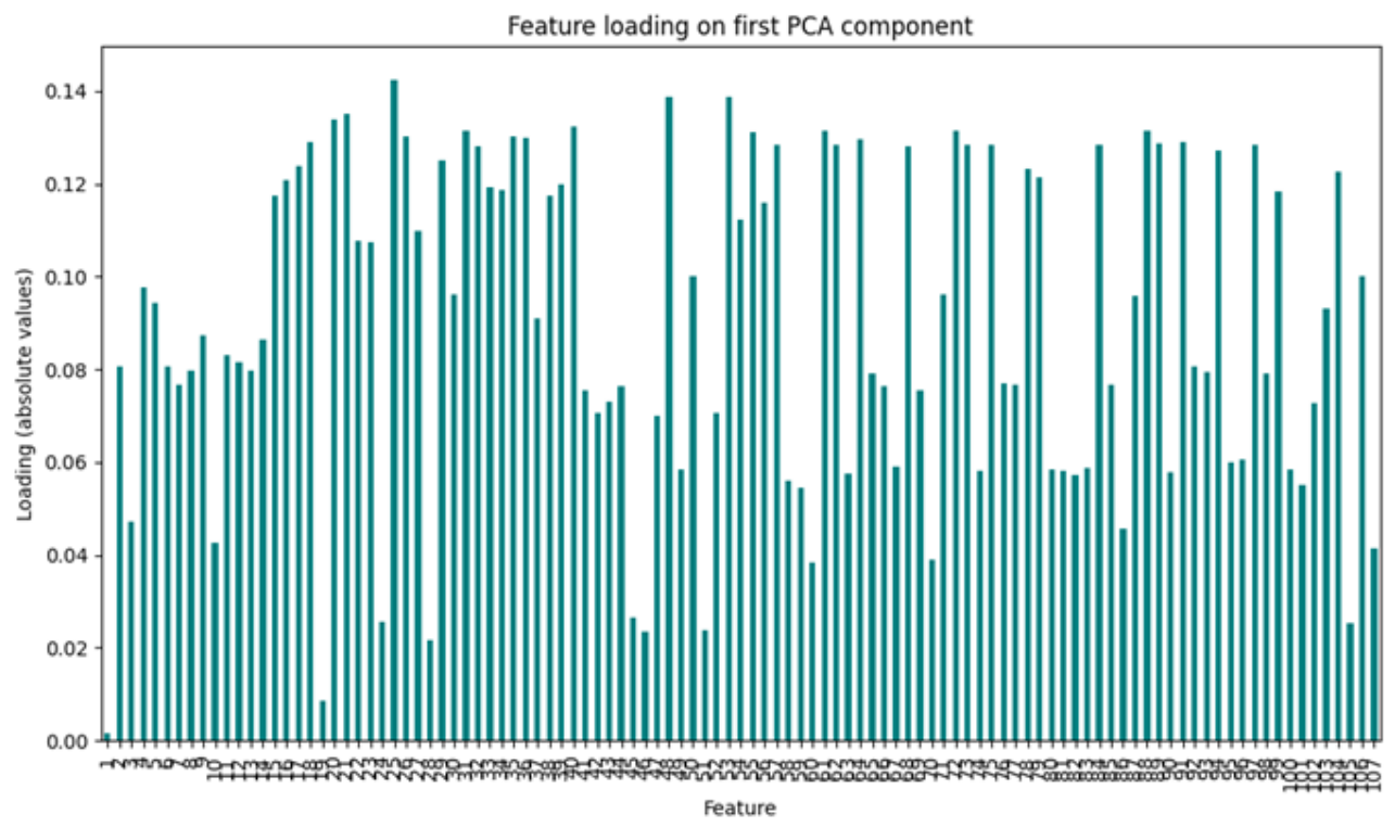
Building upon this preliminary analysis, we further explore the underlying structure of the dataset by applying PCA again, separately from training. First, we standardize the variables. Standardization ensures that each feature contributes equally to the analysis, preventing those with larger numeric ranges from dominating the variance captured by the components. The loadings of the first principal component were then examined to assess the relative contribution of each variable to this dominant direction of variance (see source code in Appendix E).
As shown in Figure A1, the absolute values of the feature loadings reveal a relatively widespread distribution, with several features exhibiting higher weights around 0.12–0.14, indicating that no single variable exclusively drives the first component. Instead, multiple features contribute meaningfully, suggesting that the dataset’s variance is shared across several dimensions rather than concentrated in a small subset of variables. This result highlights the potential complexity of the feature space and indicates that dimensionality reduction techniques such as PCA can provide a valuable step toward simplifying the representation of the data while preserving most of its variability.
Figure A1. Feature loadings of the first principal component.
Ijtm 05 00050 g0a1

Appendix D

import pandas as pd
from sklearn.decomposition import PCA
from sklearn.model_selection import train_test_split, RepeatedStratifiedKFold
 
# 1. data loading
df = pd.read_csv(“dati.csv”)
 
# pattern and target extraction
X = df.iloc[:, :-1].values
y = df.iloc[:, -1].values
 
# 2. training and test split
X_train, X_test, y_train, y_test = train_test_split(
X, y, test_size=0.2, stratify=y, random_state=42
)
 
# 3. thresholds and cross-validation
thresholds = [0.90, 0.95, 0.99]
rskf = RepeatedStratifiedKFold(n_splits=6, n_repeats=2, random_state=42)
 
# 4. PCA only on training set
for train_idx, valid_idx in rskf.split(X_train, y_train):
X_tr = X_train[train_idx]
y_tr = y_train[train_idx]
 
print(“\nNew split:”)
for t in thresholds:
pca = PCA(n_components=t)
pca.fit(X_tr)
n_comp = pca.n_components_
explained = pca.explained_variance_ratio_.sum()
print(f” n_components = {t}: number of PCA components = {n_comp}”)

Appendix E

import pandas as pd
from sklearn.decomposition import PCA
from sklearn.preprocessing import StandardScaler
import matplotlib.pyplot as plt
 
# Data loading
df = pd.read_csv(‘dati.csv’)
 
# Scaling
scaler = StandardScaler()
X_scaled = scaler.fit_transform(df)
 
# PCA
pca = PCA()
pca.fit(X_scaled)
 
# PC1 loadings
loadings = pd.Series(pca.components_[0], index=df.columns)
 
# Plot
plt.figure(figsize=(10, 6))
loadings.abs().plot(kind=‘bar’, color=‘teal’)
plt.title(“Feature loading on first PCA component”)
plt.ylabel(“Loading (absolute values)”)
plt.xlabel(“Feature”)
plt.tight_layout()
plt.show()

References

  1. Kotecha, R.; Gondi, V.; Ahluwalia, M.S.; Brastianos, P.K.; Mehta, M.P. Recent advances in managing brain metastasis. F1000Research 2018, 7, 1772. [Google Scholar] [CrossRef] [PubMed] [PubMed Central]
  2. Rades, D.; Kieckebusch, S.; Haatanen, T.; Lohynska, R.; Dunst, J.; Schild, S.E. Surgical resection followed by whole brain radiotherapy versus whole brain radiotherapy alone for single brain metastasis. Int. J. Radiat. Oncol. Biol. Phys. 2008, 70, 1319–1324. [Google Scholar] [CrossRef] [PubMed]
  3. Stelzer, K.J. Epidemiology and prognosis of brain metastases. Surg. Neurol. Int. 2013, 4 (Suppl. S4), S192–S202. [Google Scholar] [CrossRef] [PubMed] [PubMed Central]
  4. Cagney, D.N.; Martin, A.M.; Catalano, P.J.; Redig, A.J.; Lin, N.U.; Lee, E.Q.; Wen, P.Y.; Dunn, I.F.; Bi, W.L.; Weiss, S.E.; et al. Incidence and prognosis of patients with brain metastases at diagnosis of systemic malignancy: A population-based study. Neurol. Oncol. 2017, 19, 1511–1521. [Google Scholar] [CrossRef] [PubMed] [PubMed Central]
  5. Cross, N.E.; Glantz, M.J. Neurologic complications of radiation therapy. Neurol. Clin. 2003, 21, 249–277. [Google Scholar] [CrossRef] [PubMed]
  6. Lambin, P.; Rios-Velazquez, E.; Leijenaar, R.; Carvalho, S.; van Stiphout, R.G.; Granton, P.; Zegers, C.M.; Gillies, R.; Boellard, R.; Dekker, A.; et al. Radiomics: Extracting more information from medical images using advanced feature analysis. Eur. J. Cancer 2012, 48, 441–446. [Google Scholar] [CrossRef] [PubMed] [PubMed Central]
  7. Kawahara, D.; Tang, X.; Lee, C.K.; Nagata, Y.; Watanabe, Y. Predicting the local response of metastatic brain tumor to Gamma Knife radiosurgery by radiomics with a machine learning method. Front. Oncol. 2021, 10, 569461. [Google Scholar] [CrossRef] [PubMed] [PubMed Central]
  8. Jajodia, A.; Goel, V.; Goyal, J.; Patnaik, N.; Khoda, J.; Pasricha, S.; Gairola, M. Combined Diagnostic Accuracy of Diffusion and Perfusion MR Imaging to Differentiate Radiation-Induced Necrosis from Recurrence in Glioblastoma. Diagnostics 2022, 12, 718. [Google Scholar] [CrossRef] [PubMed]
  9. Cortes, C.; Vapnik, V. Support-vector networks. Mach. Learn. 1995, 20, 273–297. [Google Scholar] [CrossRef]
  10. The MathWorks, Inc. MATLAB; vR2021b; The MathWorks, Inc.: Natick, MA, USA, 2021. [Google Scholar]
  11. Pasini, G.; Bini, F.; Russo, G.; Comelli, A.; Marinozzi, F.; Stefano, A. matRadiomics: A novel and complete radiomics framework, from image visualization to predictive model. J. Imaging 2022, 8, 221. [Google Scholar] [CrossRef] [PubMed]
  12. Python Software Foundation. Powerful Object-Oriented Programming Language; Python 3.12.8; Python Software Foundation: Wilmington, DE, USA, 2024; Available online: https://www.python.org/downloads/release/python-3128/ (accessed on 13 August 2025).
  13. Wang, Y.; Duggar, W.N.; Caballero, D.M.; Vengaloor Thomas, T.; Adari, N.; Mundra, E.K.; Wang, H. Brain tumor recurrence prediction after Gamma Knife radiotherapy from MRI and related DICOM-RT: An open annotated dataset and baseline algorithm (Brain-TR-GammaKnife) [Dataset]. Cancer Imaging Archive. 2023. Available online: https://www.cancerimagingarchive.net/collection/brain-tr-gammaknife/ (accessed on 24 August 2025). [CrossRef]
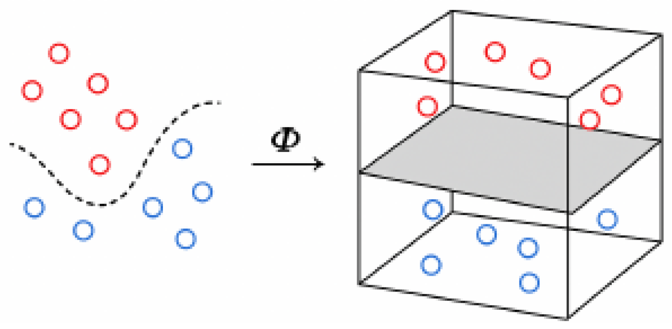
Figure 1. Φ transformation. In a higher-dimensional space, the decision boundary becomes linear.
Ijtm 05 00050 g001
Figure 2. Margin, decision boundary, and slack variables in binary (red and blue) classification in a two-dimensional (f1, f2) feature space. The arrows show the violation (slack) of outlier points.
Ijtm 05 00050 g002
Figure 3. Delimitation of ROI from an MRI image.
Ijtm 05 00050 g003
Figure 4. K-fold cross-validation, k = 4.
Ijtm 05 00050 g004
Figure 5. ROC curve on the test set.
Ijtm 05 00050 g005
Figure 6. Precision–recall–r curve on the test set.
Ijtm 05 00050 g006
Figure 7. Confusion matrix on the test set.
Ijtm 05 00050 g007
Figure 8. Reliability diagram on the test set.
Ijtm 05 00050 g008
Figure 9. Decision curve on test set.
Ijtm 05 00050 g009
Figure 10. SVM model without PCA.
Ijtm 05 00050 g010
Figure 11. SVM model with PCA.
Ijtm 05 00050 g011
Figure 12. Visual summary of radiomic features used to differentiate radiation necrosis from tumor recurrence.
Ijtm 05 00050 g012
Table 1. Radiomic features in MatRadiomics and their interpretation.
FeatureInterpretation
Shape Features
original_shape_ElongationMeasures how stretched the tumor is. A value close to 1 indicates a rounder shape; lower values indicate elongation.
original_shape_FlatnessDescribes the flatness of the shape by assessing the ratio of the minor to major principal components.
original_shape_Maximum
2DDiameterColumn
Maximum 2D diameter of the lesion measured along the column direction. Useful for assessing size in a planar view.
original_shape_SphericityQuantifies how spherical the shape is. A value closer to 1 indicates a shape close to a perfect sphere.
First-order Statistics
original_firstorder_MinimumThe lowest gray-level intensity value within the ROI.
original_firstorder_SkewnessMeasures the asymmetry of the intensity distribution. High skewness indicates deviation from a normal distribution.
original_firstorder_Total_EnergySum of squared intensity values. Reflects the total signal magnitude within the region.
Texture Features (GLCM)
original_glcm_Difference EntropyCaptures the randomness of intensity differences between neighboring voxels; higher values suggest greater heterogeneity.
original_glcm_IdmnInverse Difference Moment Normalized. Measures local homogeneity; higher values indicate more uniform texture.
original_glcm_Imc2Informational measure of correlation 2.
Assess the complexity of the texture pattern.
Texture Features (GLSZM)
original_glszm_ZoneVarianceQuantifies the variance in sizes of homogeneous zones; high values indicate varied and complex textures.
Texture Features (NGTDM)
original_ngtdm_ContrastMeasures local contrast by comparing each voxel’s intensity with its neighborhood.
original_ngtdm_StrengthRepresents the strength or coarseness of the perceived texture.
Ground Truth Label
Gold_StandardBinary label used as ground truth (e.g., 0 = control, 1 = incidence) for supervised learning.
Table 2. PCA parameter and hyperparameters in model selection.
Training ParameterValuesDescription
n_components0.90, 0.95, 0.99, NoneNumber of principal components to keep in PCA if it is an integer. Values between zero and one define the fraction of the total variance that should be preserved.
C0.1, 1, 10, 100Regularization parameter. Lower C allows wider margins with more tolerance to misclassification; higher C gives smaller margins and less tolerance to misclassification. The chosen range spans two orders of magnitude, thereby enabling the exploration of both under- and over-regularized regimes.
Kernellinear, poly, rbf, sigmoidSpecifies the kernel type. In this work, all available kernels were used, i.e., linear, polynomial, radial basis function (rbf), and sigmoid.
Degree2, 3, 4Only used with a polynomial kernel, the degree defines the complexity of the feature mapping. Degrees 2 to 4 were selected to balance representational power with computational efficiency and to avoid excessive overfitting that might arise from higher-order polynomials.
gammaauto, scaleOnly used with Radial Basis Function and polynomial kernels, auto and scale constants provide two data-dependent normalizations without introducing arbitrary constant values.
auto = 1/number of features
scale = auto/variance of input data
Table 3. Metrics with 95% confidence interval (CI) (bootstrap on test).
#MetricMean ValueCI
Accuracy0.83 ± 0.110.58–1.00
Sensitivity1.00 ± 0.001.00–1.00
Specificity0.66 ± 0.210.20–1.00
PPV0.75 ± 0.150.42–1.00
NPV1.00 ± 0.001.00–1.00
ROC-AUC0.80 ± 0.140.47–1.00
PR-AUC0.83 ± 0.140.49–1.00
Brier score0.18 ± 0.05
Table 4. Best parameters in model selection.
PCACKernel
None0.1Linear
Table 5. Radiomic features and their clinical relevance.
Feature TypeFeature NameClinical InsightPatient
Example
Confirmed Diagnosis
Textureoriginal_glcm_DifferenceEntropyHighlights heterogeneity in necrotic tissue, useful for distinguishing from more homogeneous tumor recurrence.GK_270Radiation necrosis
Shapeoriginal_shape_SphericityTumor recurrence tends to have more spherical shapes, while necrotic lesions are irregular due to tissue degradation.GK_492Radiation necrosis
First-orderoriginal_firstorder_SkewnessReflects asymmetry in intensity, typical of necrotic tissue with edema and fibrosis.GK_114Radiation necrosis
Disclaimer/Publisher’s Note: The statements, opinions and data contained in all publications are solely those of the individual author(s) and contributor(s) and not of MDPI and/or the editor(s). MDPI and/or the editor(s) disclaim responsibility for any injury to people or property resulting from any ideas, methods, instructions or products referred to in the content.