Know What You Don’t Know: Assessment of Overlooked Microplastic Particles in FTIR Images

Abstract

Assessing data analysis routines (DARs) for microplastics (MP) identification in Fourier-transform infrared (FTIR) images left the question ‘Do we overlook any MP particles in our sample?’ widely unanswered. Here, a reference image of microplastics, RefIMP, is presented to answer this question. RefIMP contains over 1200 MP and non-MP particles that serve as a ground truth that a DAR’s result can be compared to. Together with our MatLab^® script for MP validation, MPVal, DARs can be evaluated on a particle level instead of isolated spectra. This prevents over-optimistic performance expectations, as testing of three hypotheses illustrates: (I) excessive background masking can cause overlooking of particles, (II) random decision forest models benefit from high-diversity training data, (III) among the model hyperparameters, the classification threshold influences the performance most. A minimum of 7.99% overlooked particles was achieved, most of which were polyethylene and varnish-like. Cellulose was the class most susceptible to over-segmentation. Most false assignments were attributed to confusion of polylactic acid for polymethyl methacrylate and of polypropylene for polyethylene. Moreover, a set of over 9000 transmission FTIR spectra is provided with this work, that can be used to set up DARs or as standard test set.

1. Introduction

Among the methods available for the analysis of microplastics (MP), Fourier-transform infrared (FTIR) spectroscopy is currently the most frequently used method that allows chemical identification of the particles, or, in other words, determination of the particle type, here called class (e.g., polyethylene, cellulose). When combining FTIR spectroscopy with microscopy (µFTIR), spatial information of particles, such as their size and shape, is obtained additionally. Further, combination with focal plane array (FPA) detectors allows gathering of both spatial and spectral information simultaneously over a large sample area. This is called FTIR imaging and allows the swift collection of large numbers of IR spectra over a defined sample area [1]. A sample area of 1 cm², for instance, can be imaged within three to four hours, resulting in hundreds of thousands or even millions of spectra to be analyzed, depending on the instrumental parameters. This is where boon and bane of the technique lies: all spectra gathered need to be analyzed. Different data analysis routines (DARs) have been proposed, ranging from traditional database matching [2,3,4,5] to unsupervised [6,7,8] and supervised machine learning models [9,10]; an overview can be found in Weisser et al. [11]. Commonly, DARs are evaluated on a single-spectrum level, meaning that a set of test spectra is assigned to their respective types by the DAR and that these assignments are checked for correctness by the user. If the test spectra are labeled, i.e., manually assigned a type beforehand, the DAR evaluation can be carried out automatically via cross validation. While this evaluation on a single-spectrum level is unarguably essential, we will demonstrate that, in addition, the evaluation on a particle level is necessary. This is because (1) the capability of a DAR to recognize particles is in many cases based on the grouping of neighboring same-class spectra. Thus, it relies on the correlation of neighboring pixels, a parameter that single-spectrum analysis does not cover. (2) FTIR images comprise background or matrix signals that may hamper the analysis. Filtering out background signals is thus highly relevant in image classification but does not necessarily play a role in single-spectrum evaluation. (3) Even though some works have shown that their DAR correctly assigned found particles to a substance class, the DARs’ tendency to overlook particles remains unevaluated and, therefore, unknown. We thus see the following hurdles in developing and optimizing DARs for MP recognition in IR images:

(a)

Assessment of single-spectrum class assignment: lack of a standard set of test spectra.

(b)

Assessment of particle recognition: lack of a standard IR image.

(c)

Lack of objective and concise performance metrics for evaluation on the level of particles.

(d)

Comparison of DARs: lack of standard test sets and IR images.

We thus aim to contribute to solving these challenges by:

(a)

Providing a set of 9537 labeled transmission µFTIR spectra that can be used for a database, or as training/test sets for machine learning models.

(b)

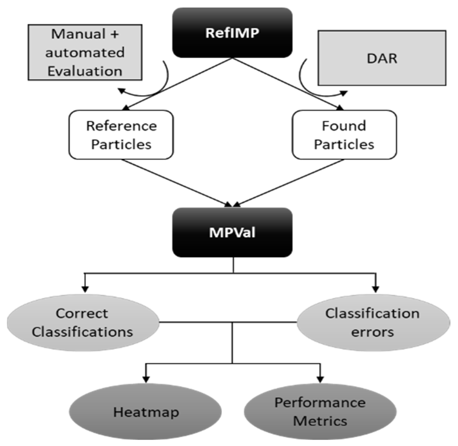
Providing a manually evaluated transmission µFTIR image of 1289 MP and natural particles that can be used as a ground truth for evaluating and optimizing a DAR on a particle level: RefIMP.

(c)

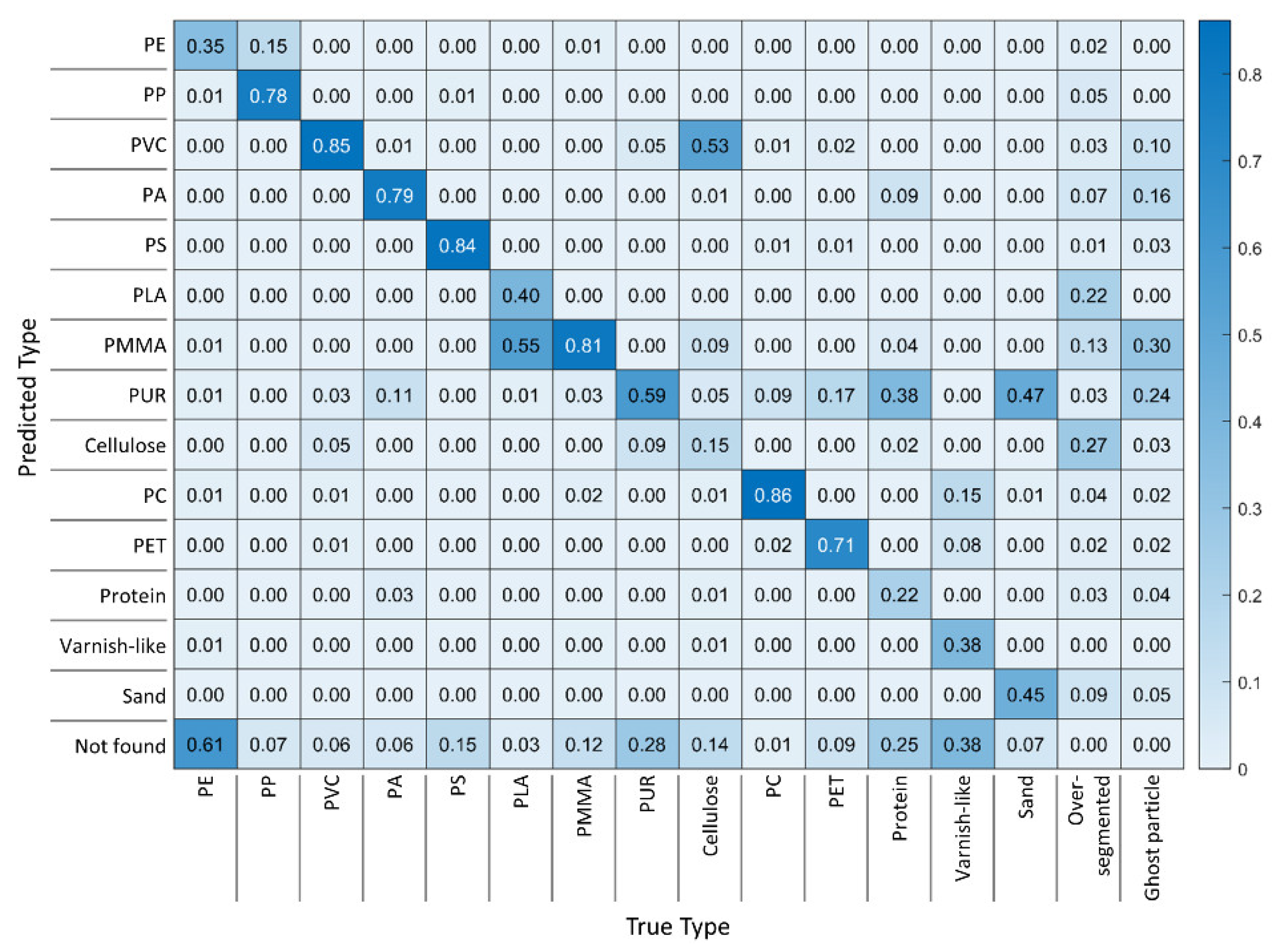
Introducing performance metrics for particle-level evaluation.

(d)

Providing an easy-to-use object-oriented MatLab^® script that automatically compares results gained using any DAR desired with RefIMP (see Figure 1).

(e)

Example hypothesis tests presented here will show how the influence of selected factors on DAR performance can be quantified using RefIMP and MPVal.

The results from the application examples are described and discussed in Section 5. Readers may directly proceed to this section. For background knowledge on the design of RefIMP, typical error types and performance metrics used here, as well as a short introduction to random decision forest models for MP recognition, readers should start with Section 2, Section 3 and Section 4.

This article focuses on FTIR images; however, the principles described here can be applied to other hyperspectral imaging techniques such as Raman and near-IR imaging, as well. Further, the general idea of establishing a known ground truth and comparing different methods using the proposed performance metrics can be applied to other MP analysis techniques such as thermoanalytical methods, too. This article does not deal with spectral manipulation techniques such as smoothing. However, these techniques can substantially influence data analysis and, therefore, we suggest to use our reference dataset to evaluate the influence of spectral manipulation techniques on data evaluation, as well. For details on spectral pre-processing, the reader is referred to Renner et al. [12].

2. An FTIR MP Reference Image: Design, Objectives and Limitations

A single reference image of course cannot represent the complexity of all imaginable MP sample types such as water, environmental or food samples together. Therefore, we started with the simplest case which is a selection of reference particles (11–666 µm) made from the most commonly found MP types: polystyrene (PS), polyethylene (PE), polyvinylchloride (PVC) (Ineos, London, UK), polypropylene (PP) (Borealis, Vienna, Austria), polyethylene terephthalate (PET) (TPL, Zurich, Switzerland), polyamide (PA) (Lanxess, Cologne, Germany), polyurethane (PUR) (from a kitchen sponge), polycarbonate (PC) (from a CD), polymethyl methacrylate (PMMA) (from a piece of Plexiglas®, Röhm GmbH, Darmstadt, Germany) and the biopolymer polylactic acid (PLA) (Nature Works, Minnetonka, MN, USA). All MP reference particles were generated through cryo-milling (Simone Kefer, Technical University of Munich, Chair of Brewing and Beverage Technology) and sieved using a 50 µm mesh stainless steel sieve. A few varnish-like particles were present unintentionally, which we decided to include in the dataset because varnish can be found in environmental MP samples, as well [13]. To represent typical natural matrix residues (non-plastic particles and fibers), we added quartz sand, protein particles (bovine serum albumin) and cellulose fibers from a paper tissue.

As was found in a broad literature screening by Primpke et al. [14], FTIR imaging for MP analysis is conducted most frequently in transmission mode with particles collected on aluminum oxide filters. Therefore, we decided to deposit the reference particles on this type of filter (Anodisc, Whatman, Buckinghamshire, UK).

The reference image contains solely reference materials deposited directly on the filter using a single-haired paintbrush under a stereomicroscope (SMZ-171-TLED, MoticEurope S.L.U., Barcelona, Spain). In pre-tests, it was attempted to prepare a suspension containing all chosen types of MP particles in equal concentrations. However, in practice, this resulted in an unbalanced distribution (types and location) of particles on the filter.

There are several manufacturers offering FTIR microscopes on the market, but according to the results of Primpke et al. [4], the instrument itself has limited influence on the data analysis. Therefore, it can be assumed that the reference image provided can be applied by others regardless of the FTIR microscope used. We conducted the FTIR measurement on an Agilent Cary 670 FTIR spectrometer coupled to an Agilent Cary 620 FTIR microscope equipped with a 128 × 128 pixel FPA detector using a 15× objective. All parameters of the measurement are given in

Table 1. Properties of the reference image RefIMP.

Property	Reference Image Provided in This Work
Plastic types	10 most frequent types, including 1 bioplastic
Matrix residues	Cellulose, proteinaceous material and sand
MP sizes	11–666 µm
MP shapes	Fragments for all types, plus cellulose fibers
Substrate	Aluminum oxide filter, 25 mm diameter, pore size 0.2 µm with PP support ring (Whatman Anodisc) placed on a BaF2 window in a customized filter holder to enhance filter flatness; for fiber samples, a second BaF2 window was placed onto the filter
Measurement mode	Transmission
Spectral range	3700–1250 cm−1
Spectral resolution	8 cm−1
Objective and projected pixel size	15×, 5.5 µm
Background scans	120 (on a blank spot of the filter)
Sample scans	30
Ground truth establishment	Pre-filtering using spectral descriptors and manual evaluation of ROIs by an expert; correction for particles found by a random decision forest model
Image size	1280 × 896 pixels, 2.72 GB (.dmd and .spe formats)

.

The images recorded were inspected carefully to identify the tiles (fields of view of the FPA detector, each ~700 × 700 µm²) most suitable for the reference images. The tiles were re-stitched (see Figure S1 in the Supplementary Information) and the resulting artificial FTIR image was named ‘RefIMP’. To enhance the accessibility of RefIMP, it is provided in the native data format *.dmd, and in addition as *.spe (converted using siMPle, www.simple-plastics.eu accessed on 10 May 2022). To keep the sample handleable by standard computers, it was designed to be in total smaller than 3 GB [4]. RefIMP was not subjected to any spectral manipulation (e.g., smoothing) and manually evaluated to create a particle ground truth as is shown in Figure 2. After having created the first DAR, its classification results were investigated to find MP particles that were overlooked during manual evaluation, but found by the model. The ground truth was corrected for these particles. The full ground truth list including the particle size distribution can be found in Figure S2 of the SI and a summary is given in

Table 2. Results from manual evaluation of RefIMP, the ground truth; size range refers to the larger Feret diameter.

Class	Quantity in RefIMP	Size Range [µm]
PE	97	11–170
PP	71	21–382
PVC	92	13–445
PA	94	18–320
PS	98	11–204
PLA	83	17–388
PMMA	124	13–320
PUR	103	17–227
PC	89	17–666
Varnish-like	10	41–100
Total MP	948	11–666
Cellulose	133	17–1890
Protein	166	11–330
Sand	42	17–292
Total non-MP	341	11–1890
Total	1289	11–1890

. Note that even though only the particle fraction <50 µm was used to prepare the reference image, particles >50 µm were present. This may be because sieving does not guarantee perfectly accurate size exclusion and, further, aggregation of particles could not be fully avoided, leading to lumps of small particles, which as a consequence appear as one big particle in the image.

3. Evaluating Data Evaluation Routines: Error Types and Metrics

Typically, results gained with any of the DARs proposed in the literature were evaluated by manual checking of the class assignments. For instance, Primpke et al. [4] stated the correct assignment rates for the particles identified by their database matching the program siMPle. However, one question remains unanswered, which is ‘How many particles were overlooked?’. This question can only be answered using a ground truth image. Therefore, a definition of typical errors that can occur during particle recognition in hyperspectral images is given in the following.

Any evaluation should comprise true positive results (TP), reflecting the samples that were correctly assigned to a type, as well as false positive results (FP), representing the wrong assignments. Moreover, correct non-assignments should be evaluated as a true negative result (TN) and incorrect non-assignments as false negative results (FN). Assessing TP/FP/TN/FN can be carried out on the level of isolated spectra by means of cross validation, where a portion of the data is repeatedly split to generate separate training and test datasets. We decided to employ Monte Carlo cross validation (MCCV), where the training–test split starts from the whole, original dataset each time [15]. Results can then be summarized in a confusion matrix and performance measures calculated. They can be categorized according to the level on which they operate. As such, class or type measures focus on only one type, while global classification measures aim to quantify the overall performance. Sensitivity and precision are well-known examples of single class measurements, representing a classifier’s ability to classify a sample correctly or to avoid false classifications for a class, respectively [15].

When assessing a DAR’s performance in an image or on the level of particles, however, performance evaluation becomes more complicated because more types of error than only FN and FP can occur, as is illustrated in Figure 3. The easiest error type is a particle falsely assigned to a class. This type of FP has a counterpart, FN, referring to the undetected class. FNs, however, also cover particles that are overlooked completely. FPs further comprise the recognition of ‘particles’ in cases where there actually is no particle, called ‘ghost particles’ here.

Another frequently observed error type is over-segmentation of particles, meaning that one particle is split into two or more ‘particles’. This can happen, for example, because of overlaying or very thick particles. The splits of over-segmented particles can all be assigned the true class, the wrong class or a mix of both.

When evaluating on a single-spectrum level, the number of predictions equals the number of samples, so the number of samples stays constant and the confusion matrix that summarizes the results is symmetric. On the level of particles, as outlined before, however, it happens frequently that more or fewer particles are found than actually present, meaning that the number of samples fluctuates. Therefore, the confusion matrix is not symmetric, complicating the calculation of the classic evaluation metrics. To solve this, we have decided to adjust the metrics to suit MP classification in hyperspectral images: sensitivities are calculated for each class, based on the number of particles of each class that are actually present in RefIMP. The arithmetic mean sensitivity, also called non-error rate (NER), thus is related to the total number of particles in RefIMP. Similarly, class precisions are based on the number of particles predicted per class and the arithmetic mean precision (Pr) refers to the total number of particles predicted. Further, we use accuracy here as the fraction of correct predictions over all reference particles.

To allow a quick and effortless evaluation of a DAR including all error types discussed above, a script was developed in MatLab^® (The Mathworks, Inc., Torrance, CA, USA), called ‘MPVal’. The script allows importing a table of reference particles (*.csv), originating either from RefIMP or an in-house reference image. The reference particles’ locations are given through their bounding boxes as shown in Figure S3. The program compares the reference particles with another table containing the center coordinates and types of the particles identified by the DAR of choice. If a found particle’s center lies within the bounding box of a reference particle and their types match, the particle is counted as a TP for this class and TN for all other classes. Figure 3 demonstrates how the different error types are dealt with. In the case of over-segmented particles, with all splits belonging to the true class, only one of the splits is counted as FP.

MPVal creates a variety of outputs in order to illuminate the evaluation results from all sides. This includes accuracy, NER and Pr, but stretches further to the sums of overlooked particles, ghost particles and over-segmentations, distinguishing ‘all true’, ‘all wrong’ and ‘true and wrong’ splits. In addition, MPVal summarizes TP/TN/FP/FN and over-segmentation factors for each class and calculates their sensitivity, precision and specificity (ability to reject samples belonging to other classes). To grant full transparency, lists are created that show which reference particle was assigned to which found particle(s) and vice versa, as well as the resulting TP/FP/TN/FN and over-segmentation factors.

When preparing RefIMP, it could not be fully avoided that, occasionally, particles were located within the bounding box of another particle. Therefore, a benchmark was established by using the list of manually labeled particles for both reference and found particle input for MPVal. This benchmark represents the best possibly achievable DAR result. Accordingly, 1185 of the total 1289 particles in MPVal are counted as TPs without over-segmentation. The remaining 104 particles are counted as ‘over-segmented with true and false types’. No other type of error was experienced in the benchmark results.

4. Random Decision Forest Classifier for MP Detection

For the automated detection of microparticles in RefIMP, we have chosen to work with random decision forest (RDF) classifiers [16]. Their application for MP classification is described in detail in Hufnagl et al. [9], so only a short introduction is given here. RDF classifiers belong to the family of supervised machine learning, meaning that to set up an RDF model, a set of labeled training data including all classes to be modeled (polymer types, natural substances and background) is necessary. Importantly, the number of labeled training spectra should be balanced across all classes [17] and the training spectra should be diverse, i.e., reflect real samples as much as possible. More precisely, this means that in the case of MP classification, the training spectra should reflect that MP spectra often suffer from a low signal-to-noise ratio, scattering effects, baseline distortion, total absorption or sample matrix residues [4,17,18,19,20]. In addition to the training data, RDF classifiers need to be provided with a set of spectral features that they can use to learn how to differentiate the classes. Examples of spectral features are the height of a band at a certain position or the ratio of the heights of two bands, see Hufnagl et al. [9]. The training data are subsampled through ‘bagging’ (bootstrap aggregating) during decision tree ‘growing’ and the features are subsampled randomly, so that each decision tree is based on a unique combination of both [16,21].

RDF classifiers were shown to yield high performance in identifying MP in FTIR and Raman spectra [10,22,23,24]. However, the performance evaluation to date has been restricted to MCCV using isolated test spectra. Any assessment on the level of particles remained rather superficial by visually checking the resulting particle image for ‘looking OK’. To the best of our knowledge, no estimation of overlooked particles has been undertaken. We aim to fill this gap with this work using RefIMP, MPVal and RDF classifiers set up in EPINA ImageLab (Epina Softwareentwicklungs- und Vertriebs-GmbH, Retz, Austria) as an example DAR. The number of trees was set to 60 and the resampling factor (training–test data split) was set to 0.60 after pre-tests (not shown). The training and test datasets are provided at https://mediatum.ub.tum.de/1656656 10 May 2022.

5. Thorough DAR Evaluation Using RefIMP and MPVal

Several aspects are known to severely influence DAR performance, such as the quality of training data for machine learning models and classification thresholds. Quantifying their influence in the context of MP recognition, however, has to date been carried out only scarcely. In order to do so, three hypotheses are tested using RefIMP and MPVal:

(1)

Masking of background pixels increases the risk of overlooking particles.

(2)

RDF models benefit from high training data diversity.

(3)

Model hyperparameters have substantial influence on the classification results.

Of course, other DARs, such as database matching, could be assessed similarly. Where applicable, the performance determined using RefIMP will be compared with the performance determined through MCCV, i.e., the meaningfulness of measuring performance on a single spectrum is critically discussed.

5.1. First Hypothesis: Masking of Background Pixels Increases the Risk of Overlooking Particles

As described in Weisser et al. [11], unsupervised machine learning techniques such as principal component analysis (PCA) seem promising to extract potential MP particles from a hyperspectral image. In brief, PCA and other techniques, such as intensity filtering, allow detection of patterns in a dataset, such as background and potential MP spectra. Only the potential MP spectra need to be analyzed further, reducing the amount of data considerably (up to 94% [6]) and thus speeding up the analysis. This includes a reduced necessity of manually correcting a result for ‘ghost particles’. However, masks arguably bear the risk of covering MP spectra unwantedly, especially when the spectra are weak or noisy. Therefore, an ideal mask covers as many pixels as possible without causing overlooking of MP particles. To the best of our knowledge, the usage of masks for real-world MP samples in the literature has never been evaluated by assessing accidentally covered MP particles but rather superficially by checking if the result ‘looks OK’ [6]. Here, we want to show how our reference image and MPVal can be used to quantify overlooking of particles as well as the occurrence of ghost particles.

Background masks were created in EPINA ImageLab using the tool Mask Creator which allows masking pixels based on the image intensity histogram. Nine masks (Mask1–Mask9) were created that cover 33% to 95% of pixels with the lowest signal intensity in the image. Another mask was created by means of PCA: based on the score plot (see Figure S4), the first and fifth PCs were found to best filter out the background spectra. However, as can be seen in Figure 4, this approach covered only a small portion of the image. Moreover, as the pixels to be masked need to be labeled manually in the PCA score plot, reproducibility of this approach can be doubted. After filtering the image with one of the masks, the unmasked pixels were subject to classification by an RDF model (trained on a dataset with 50% diversity, see Section 5.2, and default hyperparameters, see Section 5.3). The results were evaluated with MPVal. To find the best-suited mask, Figure 5 shows the percentage of overlooked and the number of ghost particles detected when using the intensity-based masks, the PCA-based mask and without any mask.

It is evident that none of the approaches reaches the benchmark of 0% overlooked particles and 0 ghost particles, meaning that the RDF classifier should be improved; yet, the results illustrate the strong influence of masks on the result: on one side, the number of ghost particles decreases with increasing size of the masked areas, as was anticipated. Without a mask, 447 ghost particles were found, decreasing slightly with the PCA-based mask and Mask1 (429 and 404, respectively). From there, the number of ghost particles drops and decreases continuously, reaching 16 with Mask9.

On the other side, the risk for overlooking particles increases with increased masked areas, as expected. While without a mask, 9.85% of particles were overlooked, Mask9, covering 95% of the image, causes 39.88% of particles to be missed. If one aims to minimize overlooking particles, either no mask or a rather small mask, such as Mask1 or the PCA-based mask in our example, should be used. It should be noted, however, that masking pixels speeds up subsequent analyses, making them attractive for high-throughput tasks. The ghost particles that are detected this way, however, will cost time during manual post-processing of the results. Aiming for a compromise that minimizes both overlooking of particles and post-processing efforts, we have chosen to use Mask2 (33% of the image covered, 10.86% overlooked and 217 ghost particles using the RDF model employed in this experiment) for all subsequent experiments.

5.2. Second Hypothesis: RDF Models Benefit from High Training Data Diversity

When training supervised machine learning models for MP classification, it has been emphasized in the literature [9] that the training data should consist not only of high-quality spectra, but contain ‘bad’ spectra, as well. We call this the ‘diversity’ of spectra here. A high diversity is expected to yield high performance for all classes and, consequently, a high global performance. Choosing the training data in the past, however, remained a somewhat subjective task as no objective metrics have been used to assess their diversity. In this section, we will show how training data diversity can be assessed and how it influences the classification result. A set of transmission µFTIR spectra of the particle types summarized in Table 2 and the Anodisc filter was sampled. Importantly, the spectra were sampled from other samples than those used to create RefIMP. Each class contains about 700 spectra with the exception of protein (475) and varnish-like (55). For model training, 80% of spectra per class were split off randomly, but stratified, while the rest served as test data. To investigate the effect of training data diversity on the classification performance, four more sets were created, in which 25, 50, 75 and 100% of spectra were replaced by copies of one spectrum for each class (see

Table 3. Training sets with varying levels of data diversity.

Diversity Level	0	25	50	75	100
% copies	100	75	50	25	0

).

Figure 6 illustrates the increase in diversity with decreasing number of copies, based on the normalized Pearson correlations (r, [0, 1]) between the spectra and corresponding references. The reference spectra were created by averaging 10 spectra of each class (see Figure S5). The closer r is to 1, the more similar are the query and reference spectrum, thus the query spectrum is considered to be of high quality, while r close to 0 stands for high dissimilarity and therefore low quality.

Note that if the 75% diversity and 100% diversity spectra underlying Figure 6 were to undergo database matching, a hard threshold, e.g., 0.70, would leave a considerable portion of spectra unassigned; while for some classes, such as PP, sand and PC, the median values are above this threshold, medians of other classes such as PE and PMMA are below. This underlines the necessity of applying class-wise thresholds rather than global thresholds in database matching, already mentioned elsewhere [2].

It was anticipated that the diversity level of the training data severely influences the RDF’s performance. However, another important model input is to be taken into account, the spectral features or descriptors (see Section 4). Thirty sets of spectral descriptors were designed, subjected to MCCV and refined until an optimized set of 161 descriptors was determined reaching the following global performances: accuracy 0.986, NER 0.958, Pr 0.987. All following RDF models were trained using this set of descriptors.

In a first step, one RDF model was trained for each training data diversity level and their performance assessed by means of MCCV. As test data, a set with 100% diversity was chosen to represent realistic conditions and avoid bias. MCCVs were performed 5-fold to account for the range of variation caused by bagged training data and feature subsampling during RDF growth [16]. The dataset 0% diversity was expected to deliver very poor results, but surprisingly, it reached mean accuracy, NER and Pr values of 0.774 ± 0.004, 0.749 ± 0.004 and 0.773 ± 0.004, respectively. With 25% diversity, the metrics jumped up to 0.974 ± 0.000, 0.946 ± 0.000 and 0.975 ± 0.001, respectively; higher diversity levels only led to very slight improvements, with maximum values at 75% diversity (accuracy 0.991 ± 0.000, NER 0.967 ± 0.000, Pr 0.992 ± 0.000). It seemed, accordingly, that RDF models can benefit from 25% duplicates in their training dataset, as opposed to our hypothesis; however, compared with the 100% diversity performance, the difference is very small and this conclusion would be premature, as shown below.

To find out how well the results from MCCV reflected the performance of the RDFs on RefIMP, the RDF results underwent evaluation with MPVal. Similar to the 5-fold MCCV, 5 RDFs were trained for each level of diversity to account for variations due to bagging of training data and subsampling of spectral descriptors during decision tree growth.

Figure 7 shows accuracy, NER and Pr determined through both MCCV and MPVal in comparison with the benchmark. Generally, MCCV underestimates the performance, showing that the manually labeled training and test data did not fully reflect the data in RefIMP. This hints towards human bias during data labeling, even though care was taken to sample a broad variety of spectral qualities. The results indicate that starting from 25% diversity, the level of training data diversity does not significantly influence accuracy and NER on RefIMP, and only for Pr was an increase observed; the 100% diversity set was the most successful with 0.681 ± 0.000, meaning that the model’s ability to avoid wrong predictions was enhanced. Still, this value could be closer to the benchmark of 1.000.

Regarding the other results from MPVal, the models with diversity levels 25–100% performed equally well: regarding the numbers of falsely assigned particles, the 100% diversity model made only 46 ± 3 false predictions, about as many as the models with 25, 50 and 75% diversity, while the 0% diversity model made 73 ± 22 false predictions. The 0% diversity model further performed the weakest in the categories ‘TP without over-segmentation, ‘FN (overlooked)’, ‘FP (ghost particles)’, and ‘Correct incl. over-segmentation’, as Figure 8 shows. Further, the standard deviations for 0% training data diversity were the highest, indicating that the robustness of an RDF model suffers when learning from low-diversity training data.

While with raising diversity, only slight performance increases were observed, the 100% diversity model stands out in the category ‘ghost particles’ that had the lowest with 204 ± 7. Compared with the other models, the 100% diversity model thus will require the least manual post-processing of the results. None of the models, however, reached more than 770 correct and non-over-segmented predictions out of the 1289 particles present in RefIMP. When including the over-segmented particles that include true predictions, i.e., that could be corrected manually afterwards, still none of the models reached more than 1105 correctly identified particles. Further, at least 124 particles were overlooked.

After assessing the RDF models, it seemed that the benchmark could not be reached. However, so far, only the global performance, i.e., the performance across all classes, has been reviewed. To draw a final conclusion, the performance should be assessed class-wise, as well. Therefore, MPVal provides an easily interpretable heat map, the diagonal of which represents the fraction of correct classifications per class, while values above and below represent false classifications. The last row (‘not found’) shows overlooked particles, and the last two columns show over-segmentation and occurrence of ghost particles per class.

For the best-performing model based on 0% diversity training data, the lowest row of the corresponding heat map (see Figure 9) shows that the most overlooked classes were PE, varnish-like, PUR and protein. Varnish-like was the class with the fewest training spectra (55) and protein was the class with the second-fewest training spectra (475), which explains the low performance [25,26]. This explanation, however, is not valid for PE and PUR with 700 training spectra each. Overlooking of these therefore most likely was caused by the lack of training data diversity or, in other words, the replicated training spectra of PE and PUR did not adequately represent the PE and PUR spectra in RefIMP. Cellulose is the class that suffered from confusion with other classes the most: 53% of cellulose fibers were mistaken for PVC by the model. PUR, apparently, was the type that caused the most false predictions, as it was predicted instead of sand, protein or as a ghost particle. Further, about a third of PMMA particles identified were ghost particles.

The best-performing model based on 100% diverse training data (Figure 10) performed better in all classes, as the values on the heat map’s diagonal show. Note that in comparison to the 0% diversity model, the share of overlooked particles decreased in all classes. Most significantly, overlooking of PE particles dropped from 61% to 12%, highlighting the importance of training data diversity. The danger of confusion is the highest for PP, about half of which was predicted as PE; similarly, PLA was taken for PMMA in every third case. Varnish-like is the class with the fewest correct predictions, which reinforces the hypothesis that with 55 training data points, the RDF model had not gathered enough information to generalize its knowledge on this class properly. With protein being the second-worst class and fewer training data points than the other classes (475 vs. 700), this conclusion is strengthened [26]. It seems that next to the potential confusion between protein and PA [25], PA may be even more likely to be mistaken for PUR.

Remarkably, cellulose was the class that suffered from over-segmentation the most, even though a BaF₂ window was placed on the fibers to hold them flat as suggested by Primpke et al. [27]. For the analysis of MP, however, it is much more important to know that no MP particles are mistaken for cellulose than to know how many cellulose particles or fibers are present exactly. As the heat map shows, cellulose was recognized correctly in 88% of the cases and seldom mistaken for other classes. PUR was responsible for most ghost particles, followed by sand and cellulose.

When we consider only the MP classes, the 100% diversity model identified most classes at a high accuracy, except for PP, PLA and varnish-like. While for the latter, the small number of training data points apparently caused the weak performance, PP and PLA training spectra were neither under-represented nor seemingly high or low quality as their normalized r values suggest (Figure 6). Taking a look at the false-color image of the particles identified in RefIMP, with examples shown in Figure 11, it can be seen that the falsely identified PE particles were located at the margins of PP particles, where the spectra were extremely distorted. Similarly, some pixels at the margin of PLA particles were mistaken for PMMA. In one case, an overlying cellulose fiber seems to have caused additional confusion. This type of error, however, can be corrected relatively easy in the Particle Editor tool.

To conclude, a highest-possible training data diversity is desirable as hypothesized, especially for maximizing the number of correctly identified, not over-segmented particles and to minimize the occurrence of ghost particles. Importantly, this conclusion could not be drawn based on MCCV, but required the assessment of both global and class-wise results from MPVal. Further, looking at the false-color map of the particles detected helped to estimate the effort necessary for manual post-processing.

5.3. Third Hypothesis: Model Hyperparameters Have Substantial Influence on the Classification Results

RDF models and other machine learning models require hyperparameters to be set by the user. They can have large influence on model performance and thus require optimization [10]. The relevant hyperparameters for RDF models as implemented in EPINA ImageLab are (1) the classification threshold detune [−0.50, 0.50], which is linked to the majority of decision tree votes that is necessary for a spectrum to be assigned to a class. Here, we have rescaled this parameter to values between 0 and 1 and call it threshold for a more intuitive understanding. Raising the threshold is expected to enhance model performance significantly in terms of correctness of the class assignments and ghost particles. If set too high, it may in turn increase overlooking of particles. (2) The minimum distance [0, 1] between the highest and second-highest vote of the decision trees. It is expected to influence the number of overlooked particles. (3) The minimum purity [0, 1], which reflects how many classes were voted for by the decision trees, thus potentially influencing the number of overlooked particles, as well. (4) The minimum neighboring correlation [0, 1], which influences the grouping of neighboring pixels to form a particle. Thus, it presumably influences over-segmentation of particles.

In a grid-search style [10], the best combination of these four parameters was searched by assessing the results from MPVal. At this point, the results gained through MCCV become irrelevant because MCCV does not take into account the hyperparameters. The experiments were conducted with the best-performing 100% diversity RDF model identified in the previous section.

Table 4. Qualitative influence of raising hyperparameters on the most important metrics derived from MPVal (↑, rise; ↓, fall; →, no influence).

Metric	Threshold ↑	Min. Distance ↑	Min. Purity ↑	Min. Neighboring Correlation ↑
Accuracy	↓	↓	↓	→
NER	↓	↓	↓	→
Pr	↑	↑	↑	→
Over-segmentation with true and false type splits	↓	↑	↓	→
Ghost particles	↓	↓	↓	→
Overlooked particles	↑	↑	↑	→
Total TPs incl. over-segmentation	↓	↓	↓	↑

summarizes the qualitative influence of each hyperparameter on the global performance metrics, the occurrence of over-segmentation with true and false type splits, ghost particles, overlooked particles and the total TPs including over-segmentation. Details are given in Figures S6–S9.

As expected, the threshold influenced the results the most, especially Pr: raising the threshold leads to strongly increased values for Pr, which can be traced back to a decrease in FP results, reflected in the reduction in ghost particles. When the threshold was set to 1.00, however, Pr became incalculable because no particle of the class varnish-like was identified. Over-segmentation was reduced, as fewer false type predictions were made. On the other hand, all other metrics deteriorated as the number of overlooked particles increased, as expected.

Minimum distance and minimum purity influenced accuracy, NER and Pr in similar ways: increasing them deteriorated accuracy and NER, which can be explained by the increase in FN results in the form of overlooked particles. Pr increased with decreasing FPs in the form of ghost particles. The same led to a reduction in over-segmentation including false type splits when raising minimum purity. Raising minimum distance, however, oppositely increased over-segmentation, reflecting that spectral quality within one particle can fluctuate.

The latter is reflected in the increased over-segmentation due to increasing the minimum neighboring correlation, as well. Apart from that, however, minimum neighboring correlation hardly influenced the results. When set to the maximum (1.00), it positively influenced the total number of TP findings. Accordingly, it was decided to set it to 1.00.

Even though minimum distance and minimum purity positively influenced Pr, their negative influence on other metrics was considerable and, consequently, it was decided to set them to their minima (0.00).

For setting the threshold, a compromise was to be found between maximum TP results and a minimum of overlooked particles, again. Testing increasing threshold values, the best compromise was a value of 0.40 with a total of 1121 out of 1289 particles correctly assigned, 48 false type assignments, 103 overlooked particles and 311 ghost particles.

6. Conclusions

RefIMP represents a state-of-the-art instrumental MP analysis technique and covers the most important substance classes. Together with MPVal, it can be used to evaluate DARs on a particle level, including intra- and inter-method comparisons. MPVal delivers concise results that illumine a DAR’s performance from all sides, reaching from its global performance to the performance for each class. Testing three hypotheses, the usability of RefIMP and MPVal was demonstrated:

(1)

background masks can strongly reduce ghost particles but, according to our results, they should not cover too much of the image to avoid overlooking of particles;

(2)

RDF models benefit from highly diverse training spectra. In particular, the share of overlooked particles was drastically reduced;

(3)

among the model hyperparameters, the classification threshold was shown to be the most important one, influencing NER, accuracy and especially Pr strongly.

Further, we have shown that when evaluating a model through MCCV, which is based on manually labeled isolated spectra, the performance on a hyperspectral image can be overestimated considerably. For example, MCCV cannot reflect the number of overlooked and ghost particles that were revealed through MPVal. Our experiments with RDF models have shown that, often, a high rate of TP results goes hand in hand with a high rate of ‘ghost particles’, i.e., particles found in places where there actually is none and that need to be deleted manually. Consequently, it is necessary to aim for a balance between high TP results and high effort for manual checking of the results. MPVal facilitates this decision by reporting on these error types in detail.

While MPVal could be used in connection with other, self-established reference images, we would also like to point out the limitations of RefIMP here. First, it cannot be guaranteed that a DAR that has shown high performance on RefIMP performs equally well on any other sample. Especially when a sample contains strongly aged MP or high amounts of matrix constituents, the DAR performance can be substantially lower. However, this does not per se lower the significance of RefIMP, as it represents the very first standard dataset, that allows comparison of DARs on a particle level. Second, using RefIMP of course only allows a statement on the polymer classes included, which cover the most important classes for MP research. However, it can easily be augmented with new sample tiles or sample tiles can be exchanged (see S1), allowing inclusion of new classes. Further, RefIMP can serve as a training object for new staff who need to get to know the varying spectra of MP classes.

To finally answer the question that has inspired us to carry out the work presented here, which is ‘How many particles were overlooked?’, we can conclude that our best RDF model overlooked 7.99% of the particles present in RefIMP. Most overlooked particles belonged to the classes varnish-like, PE and protein (12%, 12% and 18% of actually present particles of the respective class), the first and last of which were the classes with the least training data, emphasizing the necessity to provide the model with a balanced set of training data. Clearly, this leaves room for improvement; yet, this has become clear only through RefIMP and MPVal that showed how much MCCV alone overestimated the model’s performance.

References

1. Löder, M.G.J.; Kuczera, M.; Mintening, S.; Lorenz, C.; Gerdts, G. Focal plane array detector-based micro-Fourier-transform infrared imaging for the analysis of microplastics in environmental samples. Environ. Chem. 2015, 12, 563–581. [Google Scholar] [CrossRef]
2. Morgado, V.; Palma, C.; Bettencourt da Silva, R.J.N. Microplastics identification by infrared spectroscopy—Evaluation of identification criteria and uncertainty by the Bootstrap method. Talanta 2020, 224, 121814. [Google Scholar] [CrossRef] [PubMed]
3. Primpke, S.; Wirth, M.; Lorenz, C.; Gerdts, G. Reference database design for the automated analysis of microplastic samples based on Fourier transform infrared (FTIR) spectroscopy. Anal. Bioanal. Chem. 2018, 410, 5131–5141. [Google Scholar] [CrossRef] [PubMed] [Green Version]
4. Primpke, S.; Cross, R.K.; Mintenig, S.M.; Simon, M.; Vianello, A.; Gerdts, G.; Vollertsen, J. Toward the Systematic Identification of Microplastics in the Environment: Evaluation of a New Independent Software Tool (siMPle) for Spectroscopic Analysis. Appl. Spectrosc. 2020, 74, 1127–1138. [Google Scholar] [CrossRef]
5. Renner, G.; Schmidt, T.C.; Schram, J. Automated rapid & intelligent microplastics mapping by FTIR microscopy: A Python–based workflow. MethodsX 2020, 7, 100742. [Google Scholar]
6. Wander, L.; Vianello, A.; Vollertsen, J.; Westad, F.; Braun, U.; Paul, A. Exploratory analysis of hyperspectral FTIR data obtained from environmental microplastics samples. Anal. Methods 2020, 12, 781–791. [Google Scholar] [CrossRef]
7. Xu, J.-L.; Hassellöv, M.; Yu, K.; Gowen, A.A. Microplastic Characterization by Infrared Spectroscopy. In Handbook of Microplastics in the Environment; Rocha-Santos, T., Costa, M., Mouneyrac, C., Eds.; Springer International Publishing: Cham, Switzerland, 2020; pp. 1–33. [Google Scholar]
8. Shan, J.; Zhao, J.; Zhang, Y.; Liu, L.; Wu, F.; Wang, X. Simple and rapid detection of microplastics in seawater using hyperspectral imaging technology. Anal. Chim. Acta 2019, 1050, 161–168. [Google Scholar] [CrossRef]
9. Hufnagl, B.; Steiner, D.; Renner, E.; Löder, M.G.J.; Laforsch, C.; Lohninger, H. A methodology for the fast identification and monitoring of microplastics in environmental samples using random decision forest classifiers. J. Anal. Methods 2019, 11, 2277–2285. [Google Scholar] [CrossRef] [Green Version]
10. Back, H.d.M.; Vargas Junior, E.C.; Alarcon, O.E.; Pottmaier, D. Training and evaluating machine learning algorithms for ocean microplastics classification through vibrational spectroscopy. Chemosphere 2022, 287, 131903. [Google Scholar] [CrossRef]
11. Weisser, J.; Pohl, T.; Heinzinger, M.; Ivleva, N.P.; Hofmann, T.; Glas, K. The identification of microplastics based on vibrational spectroscopy data—A critical review of data analysis routines. TrAC Trends Anal. Chem. 2022, 148, 116535. [Google Scholar] [CrossRef]
12. Renner, G.; Nellessen, A.; Schwiers, A.; Wenzel, M.; Schmidt, T.C.; Schram, J. Data preprocessing & evaluation used in the microplastics identification process: A critical review & practical guide. TrAC Trends Anal. Chem. 2019, 111, 229–238. [Google Scholar]
13. Primpke, S.; Lorenz, C.; Rascher-Friesenhausen, R.; Gerdts, G. An automated approach for microplastics analysis using focal plane array (FPA) FTIR microscopy and image analysis. Anal. Methods 2017, 9, 1499–1511. [Google Scholar] [CrossRef] [Green Version]
14. Primpke, S.; Christiansen, S.H.; Cowger, C.W.; De Frond, H.; Deshpande, A.; Fischer, M.; Holland, E.B.; Meyns, M.; O’Donnell, B.A.; Ossmann, B.E.; et al. Critical Assessment of Analytical Methods for the Harmonized and Cost-Efficient Analysis of Microplastics. Appl. Spectrosc. 2020, 74, 1012–1047. [Google Scholar] [CrossRef]
15. Patro, R. Cross-Validation: K Fold vs Monte Carlo… Choosing the Right Validation Technique. 2021. Available online: https://towardsdatascience.com/cross-validation-k-fold-vs-monte-carlo-e54df2fc179b (accessed on 20 April 2022).
16. Breiman, L. Random Forests. Mach. Learn. 2001, 45, 5–32. [Google Scholar] [CrossRef] [Green Version]
17. Ivleva, N.P. Chemical Analysis of Microplastics and Nanoplastics: Challenges, Advanced Methods, and Perspectives. Chem. Rev. 2021, 121, 11886–11936. [Google Scholar] [CrossRef]
18. da Silva, V.H.; Murphy, F.; Amigo, J.M.; Stedmon, C.; Strand, J. Classification and Quantification of Microplastics (<100 μm) Using a Focal Plane Array – Fourier Transform Infrared Imaging System and Machine Learning. Anal. Chem. 2020, 92, 13724–13733. [Google Scholar] [CrossRef]
19. Renner, G.; Sauerbier, P.; Schmidt, T.C.; Schram, J. Robust Automatic Identification of Microplastics in Environmental Samples Using FTIR Microscopy. J. Anal. Chem. 2019, 91, 9656–9664. [Google Scholar] [CrossRef]
20. Renner, G.; Schmidt, T.C.; Schram, J. A New Chemometric Approach for Automatic Identification of Microplastics from Environmental Compartments Based on FT-IR Spectroscopy. J. Anal. Chem. 2017, 89, 12045–12053. [Google Scholar] [CrossRef]
21. Tin Kam, H. The random subspace method for constructing decision forests. IEEE Trans. Pattern Anal. Mach. Intell. 1998, 20, 832–844. [Google Scholar] [CrossRef] [Green Version]
22. Vinay Kumar, B.N.; Löschel, L.A.; Imhof, H.K.; Löder, M.G.J.; Laforsch, C. Analysis of microplastics of a broad size range in commercially important mussels by combining FTIR and Raman spectroscopy approaches. Environ. Pollut. 2021, 269, 116147. [Google Scholar] [CrossRef]
23. Hufnagl, B.; Stibi, M.; Martirosyan, H.; Wilczek, U.; Möller, J.N.; Löder, M.G.J.; Laforsch, C.; Lohninger, H. Computer-Assisted Analysis of Microplastics in Environmental Samples Based on μFTIR Imaging in Combination with Machine Learning. Environ. Sci. Technol. Lett. 2022, 9, 90–95. [Google Scholar] [CrossRef]
24. Weisser, J.; Beer, I.; Hufnagl, B.; Hofmann, T.; Lohninger, H.; Ivleva, N.; Glas, K. From the Well to the Bottle: Identifying Sources of Microplastics in Mineral Water. Water 2021, 13, 841. [Google Scholar] [CrossRef]
25. Schymanski, D.; Oßmann, B.E.; Benismail, N.; Boukerma, K.; Dallmann, G.; von der Esch, E.; Fischer, D.; Fischer, F.; Gilliland, D.; Glas, K.; et al. Analysis of microplastics in drinking water and other clean water samples with micro-Raman and micro-infrared spectroscopy: Minimum requirements and best practice guidelines. Anal. Bioanal. Chem. 2021, 413, 5969–5994. [Google Scholar] [CrossRef]
26. Japkowicz, N.; Stephen, S. The class imbalance problem: A systematic study. Intell. Data Anal. 2002, 6, 429–449. [Google Scholar] [CrossRef]
27. Primpke, S.; Dias, P.A.; Gerdts, G. Automated identification and quantification of microfibres and microplastics. Anal. Methods 2019, 11, 2138–2147. [Google Scholar] [CrossRef]
Figure 1. Schematic illustration of the genesis of RefIMP and application together with MPVal.
Microplastics 01 00027 g001
Figure 2. Left: µFTIR image RefIMP, intensity filtered at 2920 cm; right: color-coded particles.
Microplastics 01 00027 g002
Figure 3. Illustration of typical errors of DARs. Different colors represent different plastic types. (A) The ground truth, meaning the actually present particles. (B) A DAR result including wrong predictions and their assignments as TP, FP or FN of the corresponding classes. Not shown: complementary TN results.
Microplastics 01 00027 g003
Figure 4. RefIMP with masked pixels shown in magenta. From left to right: PCA-based mask, Mask2 and Mask6 (covering 65% and 88% of pixels, respectively, based on their signal intensity).
Microplastics 01 00027 g004
Figure 5. Left side: relation of overlooked and ghost particles depending on background masks; right side: % area of RefIMP covered by the masks.
Microplastics 01 00027 g005
Figure 6. Normalized Pearson correlations (y axes) of the training data at different levels of diversity (x axes) with their respective references.
Microplastics 01 00027 g006
Figure 7. Accuracy, NER and Pr determined through MCCV and MPVal for the benchmark and training sets with 0–100% diversity.
Microplastics 01 00027 g007
Figure 8. Influence of training set diversity on correctly predicted particles that are not over-segmented, overlooked particles, ghost particles, correctly predicted but over-segmented particles and incorrect predictions.
Microplastics 01 00027 g008
Figure 9. Heat map of the results from an RDF model with 0% training data diversity compared with the ground truth of RefIMP.
Microplastics 01 00027 g009
Figure 10. Heat map of the results from an RDF model with 100% training data diversity compared with the ground truth of RefIMP.
Microplastics 01 00027 g010
Figure 11. Left side: example for FP PE particles (blue) at the margins of a PP particle (magenta). Right side: example for FP PMMA particles (purple) at the margins of a PLA particle (yellow) and partly covered by a cellulose fiber (green, only partly recognized).
Microplastics 01 00027 g011