The Raman Spectroscopy Approach to Different Freshwater Microplastics and Quantitative Characterization of Polyethylene Aged in the Environment

Abstract

The aim of this paper is to contribute to the investigation of microplastics reaching the Baltic Sea with freshwater input. The scope of the paper was to analyze samples from several locations with different environmental characteristics. First, samples from urban areas differing in their degree of urbanization, a forest, a river and its watercourse were examined. Secondly, the ageing quantitative and qualitative characterization is discussed. Spectral techniques are crucial in identifying polymers, but the signal itself constitutes a valuable source of the crystallinity and density parameters of the polyethylene materials. The study indicates that polypropylene, polyethylene, polycarbonate and polystyrene are the most common types of microplastics in the investigated areas.

1. Introduction

Microplastics are particles of synthetic material with irregular shapes and dimensions with at least one linear dimension < 5 mm [1,2], whereas nanoplastics (NP) are <100 nm (some authors also include debris < 1 µm). Microplastics (MP) are classified based on physicochemical properties, such as shape (fibres, fragments, granules), size and material [3]. A distinction is made between primary microplastics, which are produced with the intention of a specific application (granules, industrial abrasives, etc.), and secondary microplastics that are produced by the fragmentation or damage (abrasion, delamination, weathering) of larger objects (fragments of fishing nets, synthetic bags, etc.) [4]. Fragmentation and damage are caused by wastewater treatment, sunlight and biological processes [5,6,7]. Much of the plastic produced is not recycled and ends up in the environment, where it poses a serious threat to animals [8]. It is estimated that approximately 4.8–12.7 million of tonnes of plastic pollution enters the global ocean annually [9]. Rivers are the dominant source of microplastics in the seas [10,11]. Approximately 70–80% of the pollution found in the seas comes from land [12,13]. An estimated 5.25 trillion MP and NP are in the global ocean [14]. Despite studies conducted in different sections of the Vistula River, including near the estuary and on the coast and in the Baltic Sea, the detailed influence of the Vistula River on microplastic concentrations in the Baltic Sea is not known [15].

MP particles enter aquatic ecosystems through wind, surface runoff and direct sewage outflows [16,17]. Current wastewater treatment technologies show up to a 90% efficiency in removing microplastic pollutants [14]. Laundry, municipal and industrial wastewater are the primary sources of toxic substances in the world ocean [18,19]. MP particles have been identified in water and sediments in numerous rivers worldwide [20,21]. Many studies indicate that increased concentrations of MP in water and sediment are closely related to proximity to heavily populated areas, industrial centers and sewage treatment plants [15]. For example, sediment and water samples collected from the Vistula River in the Warsaw metropolitan area were significantly more contaminated with MP than samples deposited near the mouth and downstream [15,22].

Additionally, sediments collected near the mouth of the Vistula were the most contaminated among all deposited samples in the Gulf of Gdansk. This indicates that the Vistula River provides significant amounts of MP that may accumulate near its mouth. The variation in MP abundance along the Vistula may be explained by Warsaw being a densely populated city with industrial areas and sewage treatment plants. This hypothesis is supported by a study on the Rhine River, where MP concentrations along and across the river were highly variable but reached their maximum in the Rhine-Ruhr metropolitan area [13]. MP concentrations increased along the river, and the micropollutant profile reflected the number of cities, their population and the industrial centers. Analysis of MP concentrations conducted on the Pearl River (China), where Hong Kong, located near its mouth, has become a ‘hot spot’, suggests similar conclusions [23]. A similar phenomenon is observed in the Atoyac River, near an industrial complex and densely populated city of Puebla [24]. Additionally, it was shown that MP abundance in samples collected from urban areas on the Tamew River was 65% higher than in samples from rural areas.

Previous studies indicate that areas such as Warsaw may be a significant source of MP pollution. In addition to proximity to heavily populated areas, industrial centers and wastewater treatment plants, MP abundance is influenced by hydrodynamic characteristics (e.g., currents, channel geometry, flow velocity, standing water zones), geomorphological characteristics, weather events (e.g., flooding) and MP properties [21], [12,13,20,25]. Lin et al. (2018) found that hydrodynamic conditions can influence the different spatial distribution of MP at sampling sites. Some of the transported MP particles may temporarily accumulate in either the water column or sediments [25,26]. MP sinking may also be associated with biofouling, erosion-induced changes in MP density and particle adhesion to their surfaces [27,28]. It was observed that a low river velocity associated with the season [29] and undisturbed flow influence the increase in MP abundance in fine sediments.

In the example of the Vistula River, no apparent increase in MP abundance was observed in water and sediment samples, consistent with the river current. Similar differences in spatial distribution between water and sediment samples were found on the Antuă River [25]. Water samples from Wilanów Zawady beach, located in the southern, less urbanized part of the city, were more contaminated with MP than samples collected from the right bank of the Vistula near the “South” sewage treatment plant and the mouth of the Wilanowka tributary. This could be because the velocity of Vistula flow in the vicinity of the “South” sewage treatment plant (approximately 0.9–1 m s—1 in July 2011) was higher than in the vicinity of the Wilanów Zawady beach (approximately 0.3–0.5 m s—1 in July 2011) and, as a result, the faster flow of the Vistula may have contributed to the lower concentration of MP in the water samples [29,30,31]. However, MP abundance in sediments was highest in samples collected near the “South” wastewater treatment plant. Such a high abundance of MP in sediments at this location may have been caused by hydrological conditions (presence of arrowheads on the right bank of the Vistula causing strong current turbulence) and the probable supply of MP from the Wilanówka tributary and the sewage treatment plant.

Additionally, the complex sedimentary conditions influenced the various grain size distribution, which was not recorded in the other locations [13,16,29,30]. The highest abundance of MP in water was recorded for samples from the beach at the Prince Józef Poniatowski Bridge, located in the city’s more populated, central part. The faster flow of the Vistula may have influenced the lower concentrations of MP in sediments in the city center [15]. The hypothesis may be supported because significant amounts of coarse sand were collected at this site, indicating that smaller sediment particles were transported downstream with MP [21]. Another reason for the different abundance of MP in the sediment compared to other studies may be the different seasons in which samples were taken. Due to a reduced river flow, more MP particles may be deposited along the channel during the winter season. In all reported studies, the riverbanks and sites near freshwaters were not considered. Thus, we would like to provide insight into solid phase contamination in direct vicinity of freshwater sources within this research.

The qualitative and quantitative identification of microplastics is possible using spectral techniques. They allow for rapid measurements, have a high spatial resolution and the degradation of samples only takes place because of the excessive intensity of the laser beam. Raman spectroscopy and Fourier-transform infrared spectroscopy (FTIR) are complementary methods. A low-intensity signal or one that is impossible to register with the FTIR technique appears in the Raman spectrum, and vice versa. Therefore, spectroscopy is one of the most versatile MP identification and characterization approaches. Although FTIR [32] exhibits fewer problems with the self-luminescence of samples, Raman spectroscopy [33] has a better spatial resolution, and the potential to collect signals in higher frequencies is also not to be neglected. Many studies focus on identifying the MP type correctly, especially in complex environmental matrices. However, relatively little is known [33,34] about the proper quantitative approach to those spectra [35]. Preliminary results mainly indicated the following problems: a proper background cut off, the need for deconvolution that would separate the bands and have a physical meaning in peaks description, a lack of standards in order to make a reliable statistic and an ageing model with correlation to the spectroscopic signal.

This work provides a preliminary overview of various sources directly influencing freshwater MP. Moreover, the approach to better PE characterization is proposed and discussed. The freshwater samples were chosen as their impact on marine microplastics is direct and significant, but data are still scarce [36].

2. Materials and Methods

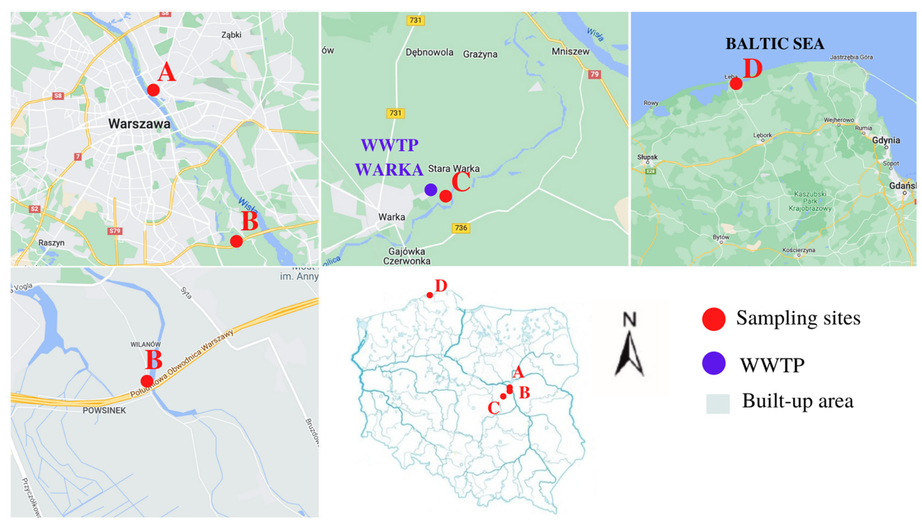
2.1. Study Area and Sample Collection

Samples for analysis were taken from four different locations in Poland, as shown below (Figure 1): (A) the shore of the Vistula River near the Śląsko-Dąbrowski Bridge, which is located in the more populated, central part of Warsaw; (B) the shore of the canal flowing into the Wilanówka River, which is located in a moderately built-up part of Warsaw, near a highway; (C) the forest area near the Warka wastewater treatment plant (WWTP), where the average population density is 444 person/km²; (D) a protected area of the Słowiński National Park, which is relatively intensively used for tourism. Sites A, B and C were sampled in summer, between May and July, whereas site D was sampled in autumn, after a storm. The selection of sites was guided by the degree of urbanization, population density and proximity to WWTP. Contaminants in forest areas may flow down to the nearest stream together with rainfall and silt and be further transported to the river (Pilica). At the same time, there is less risk that the micropollutants present are synthetic fibres from washing clothes.

The sampling area was chosen randomly as the 1 m × 1 m square. The sampling depth was below 5 cm (mainly surface debris, all fractions in 0–1 cm of depth and those partially buried deeper if present on the surface). In the rare cases where the fragmentation of macroplastics was already visible (by numerous pieces of the same material in its vicinity), the “main” object was also taken, although being >5 mm.

2.2. Identification by Raman Spectroscopy

In this study, Raman spectroscopy was used as an efficient method for the analysis. The technique allows for the identification of micropollutants with dimensions greater than 1 µm (source). Qualitative studies were performed at the Centre for Biological and Chemical Sciences, University of Warsaw (Warsaw, Poland). Spectra were obtained using a Thermo Scientific DXR Raman Microscope equipped with an optical microscope. The spectroscope operated at four laser line lengths: 532 nm, 455 nm, 633 nm and 780 nm. The study was performed using two laser lines: 532 nm and 633 nm. The maximum laser power used was 10 mW. Some measurements were carried out at lower powers to prevent sample degradation and reduce luminescence. The spectroscope was equipped with a 10 mm objective with a diaphragm of 50 µm aperture. The US National Oceanic and Meteorological Service (NOAA) recommends thoroughly cleaning all inorganic and organic contaminant samples before analysis. All samples were also mechanically cleaned of any lingering sand on their surface before recording spectra in the following study. This step consisted of gentle dust removal, rinsing in mill-Q water and filtration on a chromium-nickel net (25 µm). The OMNIC database extended by authors during the last seven years (>10,000 records) was used for qualitative identification. As a double-check, the SLoPP data and the Renishaw database were controlled.

2.3. Quantitative Signal Analyses

Apart from the raw spectra, the OMNIC standard background cut off was used and compared with the proper ORIGIN or Python processing. All signal analyses were carried out using the Python scripts designed for that purpose and using the following libraries: matplotlib, NumPy, scipy, spectrapepper. In addition, the authors used four different background approaches to enhance the accuracy of ageing modeling. Those included:

▪

OMNIC standard;

▪

Adaptive iteratively reweighted penalized least squares (AIRPLS, named A);

▪

Asymmetrically reweighted penalized least squares (ARPLS, named B);

▪

Asymmetric least squares smoothing (ALSS, named C) and its updates.

The second and fourth approaches were the best, respectively, noted as A and C. However, the asymmetrically reweighted penalized least squares background too deeply penetrated peaks in a non-representative physically way, which creates systematic errors, such as the negative values in ageing parameters. That is why it was not considered further for numerical modelling of those data.

3. Results and Discussion

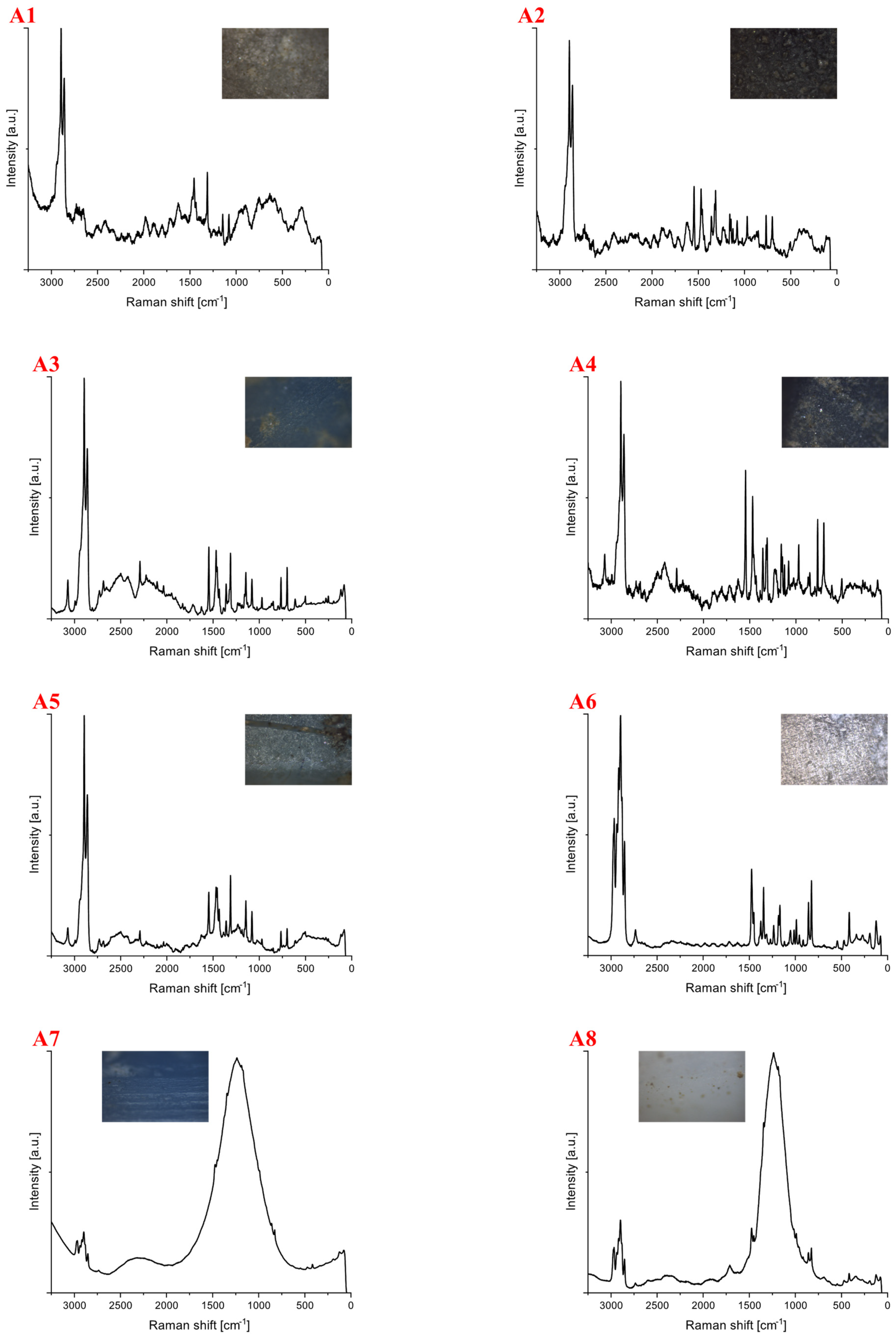
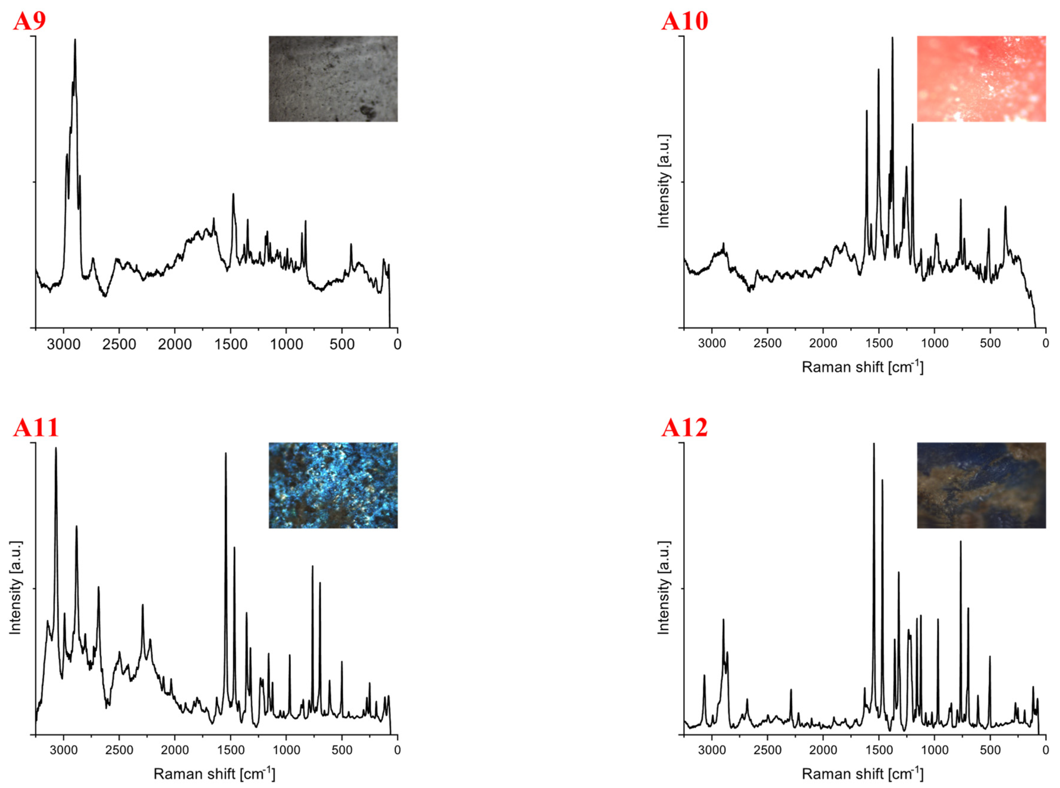
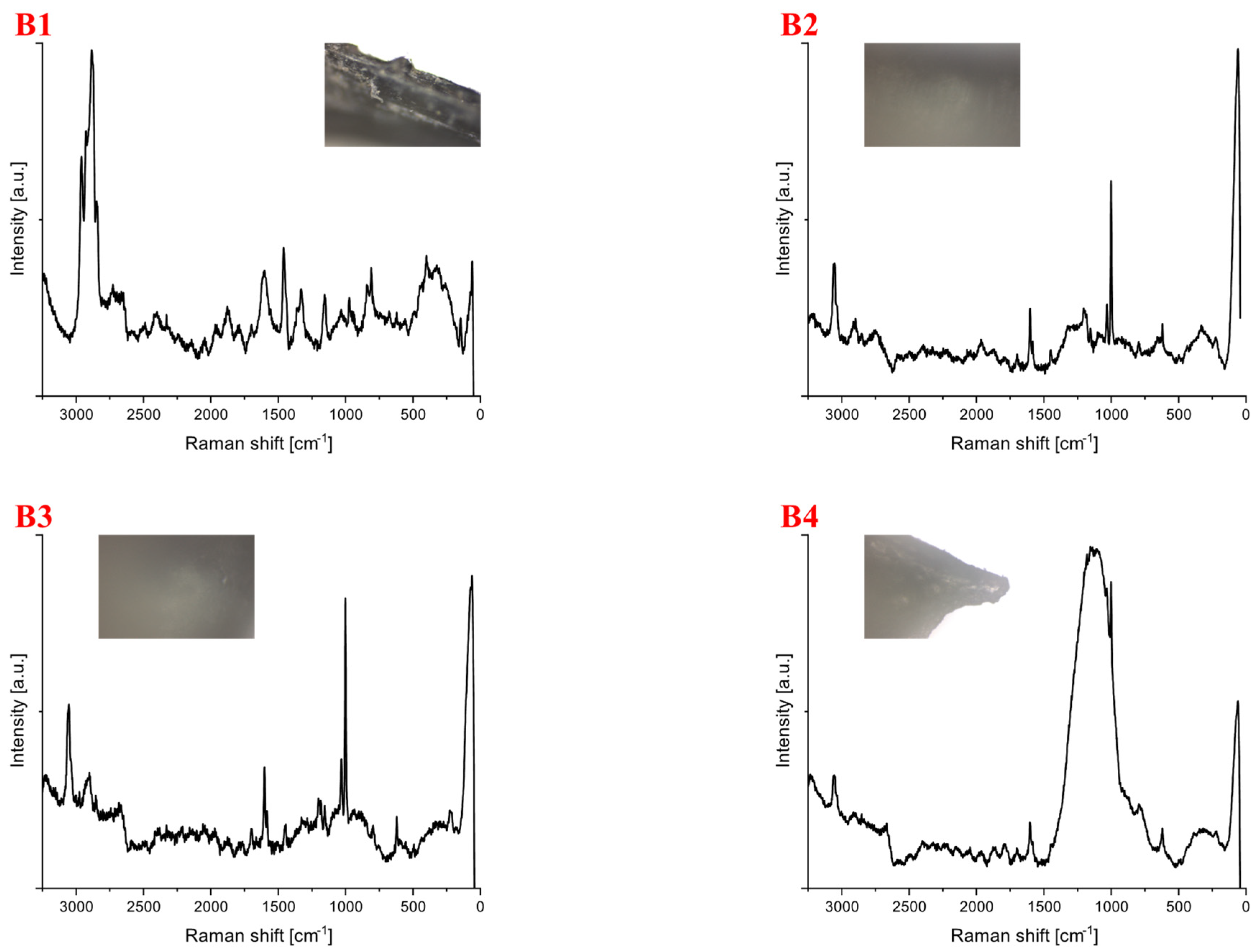
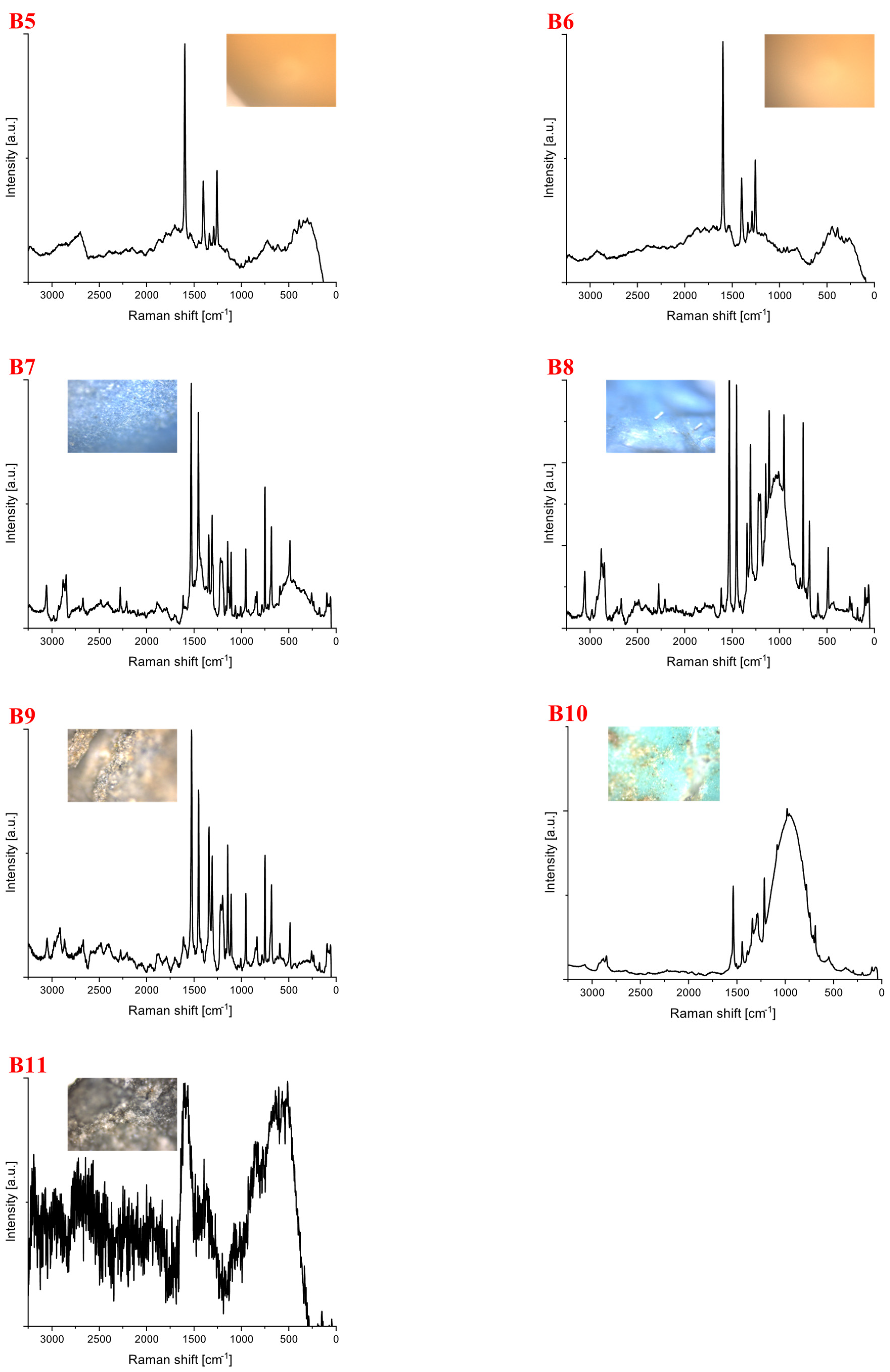
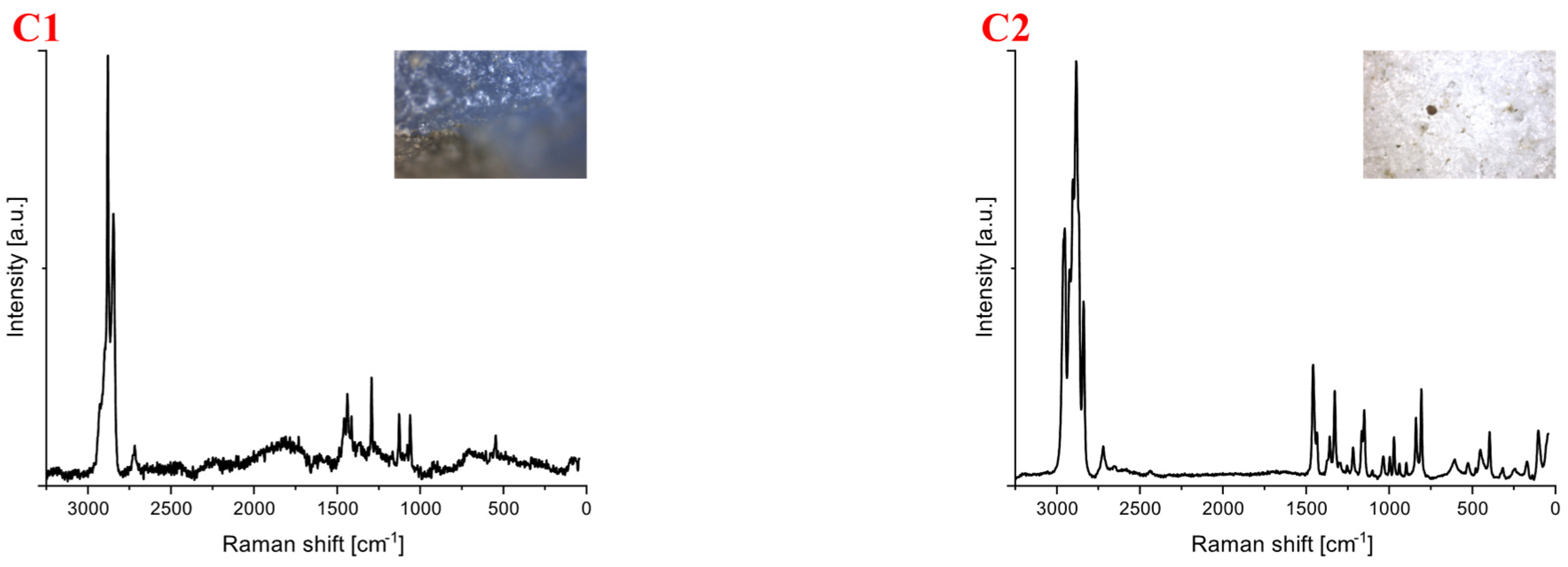
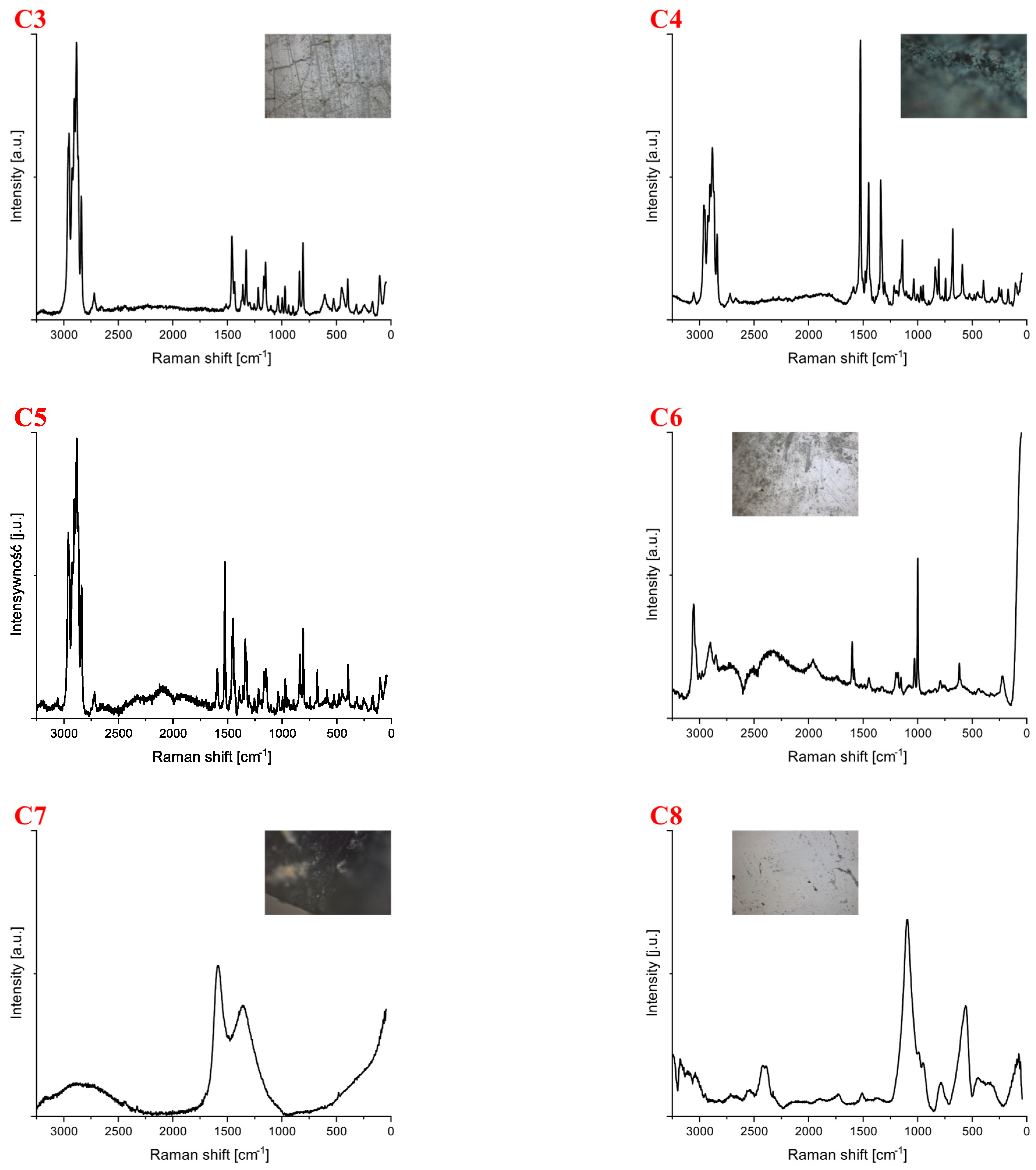
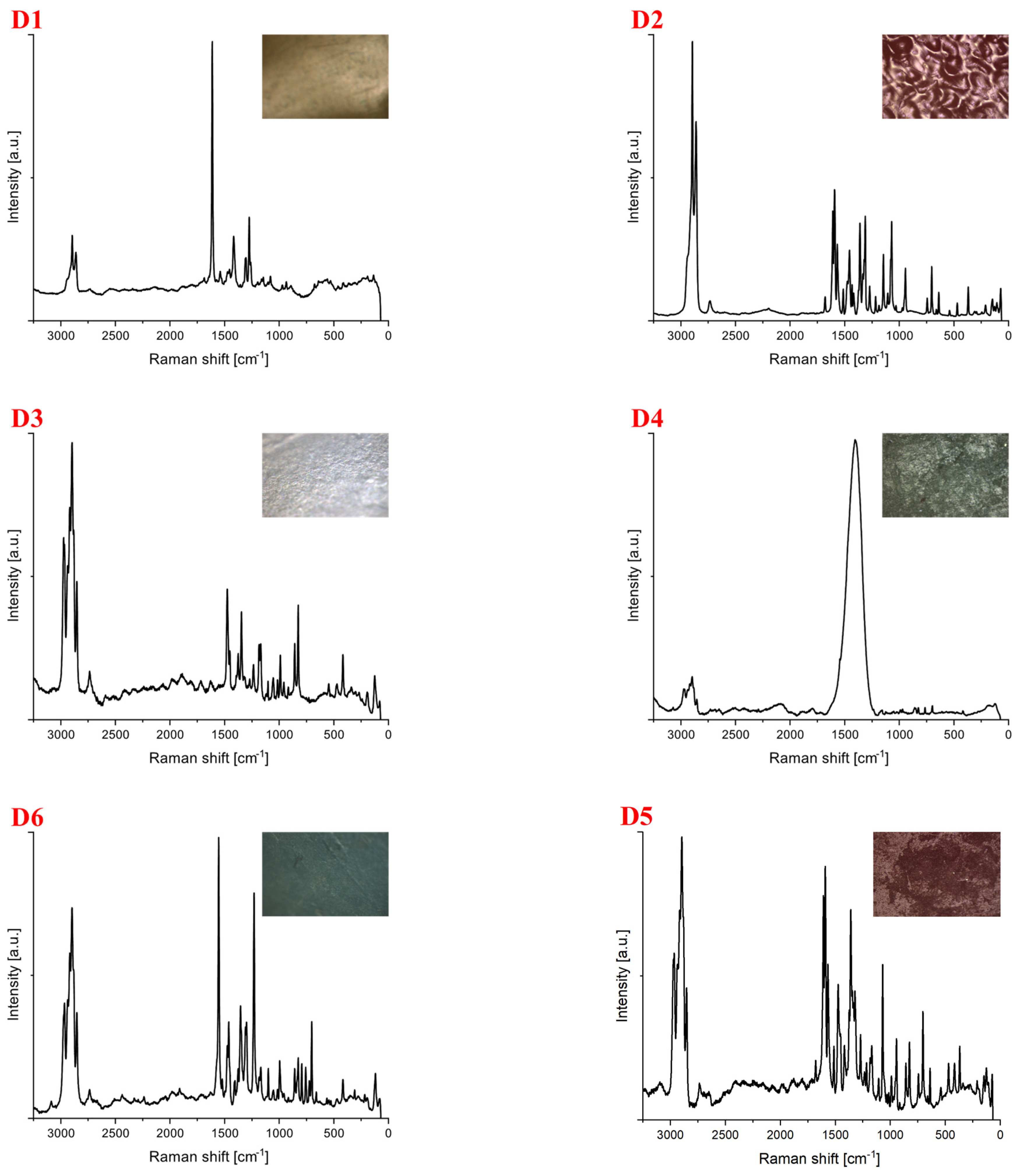
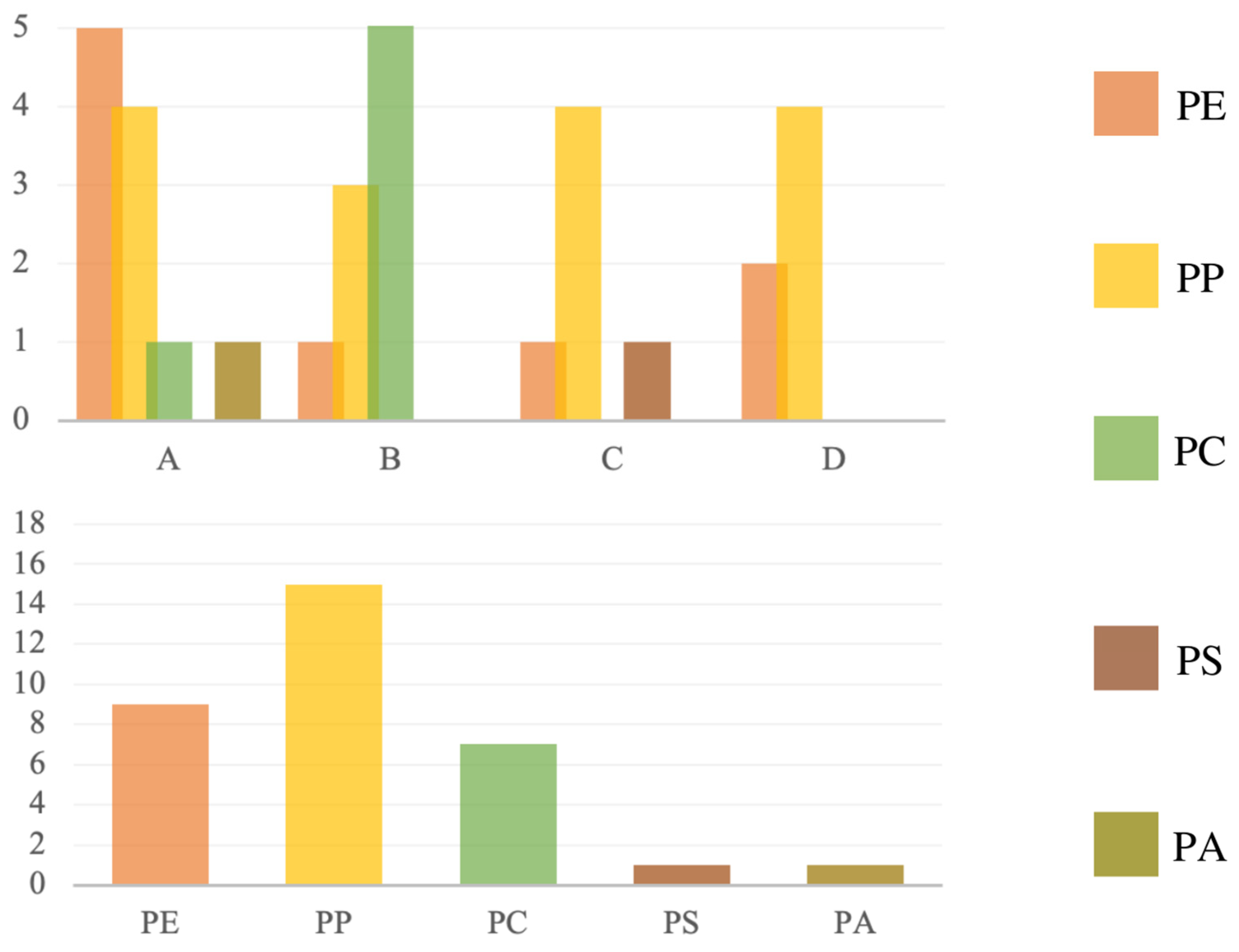
3.1. Qualitative Characterization of MP by Raman Spectroscopy

Spectra for samples collected from the shore of the Vistula River near the Śląsko-Dąbrowski Bridge (A) are shown in Figure 2. For this location, 21 samples were collected, of which, 9 showed luminescence and could not be further identified. The identified plastics were of different shapes and colors (

Table 1. Characterization of polymers at stand A.

Polymer Type	Signature	Color	Shape	Size
Polyethylene	A1	White	foil	upper limit
	A2	Blue	fragment (rectangular)	upper limit
	A3	Red	fragment (irregular)	upper limit
	A4	Blue	fragment (irregular)	5 mm × 2 mm
	A5	blue	fragment (irregular)	2 mm × 1 mm
Polypropylene	A6	white	fragment (rectangular)	upper limit
	A7	white	cylindric, lollipop stick-like	upper limit
	A8	blue	cylindric, lollipop stick-like	upper limit
	A9	colorless	foil	upper limit
Polyamide	A10	red	foil	upper limit
Polycarbonate	A11	blue	foil	3 mm × 2 mm

). One sample was not identified despite the recorded spectrum (A12). Among the tested samples, polyethylene (24%), polypropylene (19%), polycarbonate (5%) and polyamide (5%) were identified. The test was performed with a laser line of 633 nm, and the number of repetitions for all spectra was 50. The sample exposure time and the laser power were changed, which was 8 mW for most measurements. In the case of the A11 spectrum, a laser power of 2 mW was used. Spectra A1 to A5 were identified as polyethylene. A qualitative analysis of the polymers can be based on visual differences in signals from the stretching vibrations of the -CH chain at 3200–2800 cm⁻¹. The polymer region shows two characteristic bands at ~2882 cm⁻¹ and 2848 cm⁻¹, corresponding to asymmetric stretching in the crystalline phase and symmetric stretching in the amorphous phase [37].

Polymer ageing is inferred from the ratio of amorphous to crystalline domains. Enhanced background noise and autofluorescence are frequently typical features of naturally weathered materials. It is the collateral effect of the organic and inorganic matter presence. The most enhanced background noise characterizes spectrum A1 compared to the other PE spectra. On this basis, it can be assumed that this is probably the oldest or most aged PE. However, additional quantitative analysis is needed (as described in Section 3.3) to confirm it. In addition, bands for oxygen-containing functional groups (mainly the C=O stretching at 1643 cm⁻¹) are an essential indicator of ageing as they occur mainly due to oxidation.

The distinction between high-density polyethylene (HDPE) and low-density polyethylene (LDPE) is based on comparing the relative difference in intensity between asymmetric vibrations in the crystalline phase and symmetric vibrations in the amorphous phase. The degree of crystallinity is proportional to the density of the polymer. HDPE has a higher number of crystalline domains compared to amorphous domains than LDPE. All recorded spectra for polyethylene (A1–A5) are most likely not LLDPE, as the signal from asymmetric stretching vibrations (~2882 cm⁻¹) has a higher intensity than the signal for symmetric stretching vibrations (2848 cm⁻¹). In addition, in the range 1500–1200 cm⁻¹, the band coming from vibrations of the -${\mathrm{CH}}_2$, the group in the crystalline phase, has a higher intensity than the band coming from vibrations of the -${\mathrm{CH}}_2$, a group in the amorphous phase.

Samples A6 to A9 were identified as polypropylene. The spectrum marked A7 belongs to new polypropylene. The other samples representing PP are either older or more aged. Samples A10 were identified as polyamide, whereas spectrum A11 was assigned to polycarbonate. The Raman spectrum of PA 6, the most common polyamide, exhibits the following bands: -CC deformation at 643 cm⁻¹, -CCO stretching at 935 cm⁻¹, -CC skeletal stretching at 1066, 1084 and 1132 cm⁻¹, CN stretching and -NH bending of amide III at 1298 cm⁻¹, -CH₂ twisting at 1308 cm⁻¹, -CH₂ bending at 1448 cm⁻¹ and -CH stretching at 2942 cm⁻¹. At first glance, this last peak suggests the need for further examination of the presence of PA. Sample A12 is not identified.

Spectra for samples collected from the canal’s shore flowing into the Wilanówka river (B) are shown in Figure 3. For this location, 18 samples were collected. In the case of 7 of them, the phenomenon of luminescence occurred. Among the identified samples, polycarbonate constituted the most considerable part (33%), followed by polystyrene (17%) and polypropylene (6%). The identified plastics were of different shapes and colors (

Table 2. Characterization of polymers at stand B.

Polymer Type	Signature	Color	Shape	Size
Polyethylene	B1	black	Foil	upper limit
Polypropylene	B2	white	fragment (fibrous)	upper limit
	B3	white	fragment (irregular)	5 mm × 4 mm
	B4	white	fragment (irregular)	upper limit
Polycarbonate	B5	yellow	fragment (irregular)	4 mm × 2 mm
	B6	yellow	fragment (irregular)	4 mm × 3 mm
	B7	blue	foil	upper limit
	B8	blue	foil	4 mm × 1 mm
	B9	blue	foil	upper limit
	B10	green	foil	upper limit

). Spectroscopic studies were carried out at a laser line of 633 nm, except for the measurement carried out for the sample whose spectrum was labeled B11 (532 nm). The number of repetitions, sample exposure time and laser power varied (4 mW–8 mW). The spectrum marked B1 represents polypropylene. Spectra B2, B3 unambiguously indicate polystyrene because, in the range of tensile vibrations -CH (3200–2800 cm⁻¹), there are characteristic bands that are easy to identify. At a frequency of approximately 1000 cm⁻¹, a signal appears, typical of bending vibrations -CH in the aromatic ring. The spectrum taken for sample B4 is characterized by significantly increased background noise and autofluorescence but most likely represents polystyrene.

The spectra labeled B5 to B10 represent polycarbonate. In all spectra, there was a signal at a frequency of ~1611 cm⁻¹, which corresponds to the stretching vibration of the phenyl ring [38]. The spectra of polycarbonate in the polymer range (3200–2800 cm⁻¹) are like those of polystyrene. In the polystyrene spectra, there is a high-intensity band at ~1611 ${\mathrm{cm}}^{-1}$, corresponding to the -CH bending vibration in the aromatic ring, not present in the spectra for polycarbonate. Samples labeled B5 and B6 represent the same compound because their spectra and optical microscope images are very similar. A similar situation exists for the samples labeled B7 and B8.

The spectrum of B11 was not identified due to the presence of significant background noise.

Spectra for samples collected near the forest area near the wastewater treatment plant in Warka (C) are shown in Figure 4. For this location, 12 samples were collected, of which, 4 showed the phenomenon of autofluorescence. The identified samples included polypropylene (33%), polyethylene (8%), polystyrene (8%), cellulose (8%) and carbon (8%). The identified plastics were of different shapes and colors (

Table 3. Characterization of polymers at stand C.

Polymer Type	Signature	Color	Shape	Size
Polyethylene	C1	blue	fragment (irregular)	4 mm × 3 mm
Polypropylene	C2	white	fragment (irregular)	upper limit
	C3	white	fragment (irregular)	3 mm × 2 mm
	C4	blue	Foil	5 mm × 4 mm
	C5	blue	Foil	4 mm × 2 mm
Polystyrene	C6	white	fragment (irregular)	5 mm × 4 mm
Carbone	C7	black	fragment (irregular)	upper limit
Cellulose	C8	white	fragment (irregular)	4 mm × 3 mm

). Spectroscopic measurements were performed at a laser line of 532 nm. The exposure time of the samples and the number of repetitions varied throughout the experiment. The laser power for most measurements was 10 mW, except for C1 (8 mW). The spectrum labeled C1 represents polyethylene, and the subsequent ones (C2–C5) indicate polypropylene. Subsequent designations belong to C6-polystyrene, C7-carbon and C8-cellulose. At a frequency of approximately 1000 cm⁻¹, a signal typical of -CH bending vibrations in the aromatic ring appears. This band is very characteristic of polystyrene.

Spectra for samples collected from the area of the Słowiński National Park (D) are shown in Figure 5. For this location, 12 samples were collected, of which, the identification of 6 was not possible because of autofluorescence. Polypropylene constituted the most extensive part (33%), followed by polyethylene (17%). The identified plastics were of different shapes and colors (

Table 4. Characterization of polymers at stand D.

Polymer Type	Signature	Color	Shape	Size
Polyethylene	D1	yellow	foil	upper limit
	D2	Red	spherical, cap-like	upper limit
Polypropylene	D3	white	foil	upper limit
	D4	green	fragment (irregular)	upper limit
	D5	Red	fragment (rectangular)	upper limit
	D6	green	fragment (cylindric)	upper limit

). Spectroscopic studies were performed at a laser line of 633 nm. Only the exposure time of the samples was changed during the measurement. The laser had a power of 50 mW, and the number of repetitions was 50. The symbol D1 denotes the polyethylene spectrum. Samples D2 to D6 were identified as polypropylene.

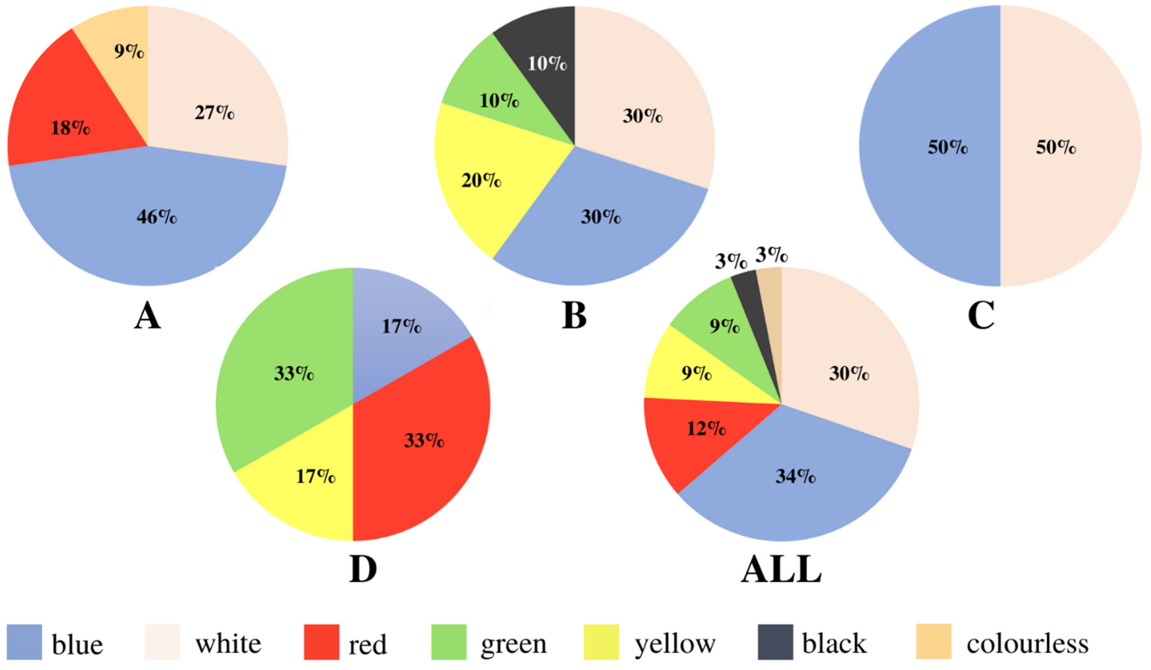
3.2. Characteristics of the Morphology

The most abundant particle color was blue, representing 34% of all identified plastics (Figure 6). The proportion of white particles was also significant (30%). Red, yellow, green, black and colorless particles were the least frequent. Although the films were characterized by all of the colors mentioned above, only colorless particles were absent among the fragments. The most varied particle colors were at position B. the minor color variation was observed at location C, where blue and white particles predominated. For sites A and D, the color distribution of particles was similar, with blue particles dominating at site A and the same number of green and red particles present at site B.

The most significant number of particles found at sites were not classified as microplastics. Instead, the most significant number (52%) of all plastic particles identified were fragmented (Figure 7), which are most commonly formed by the degradation of larger objects made from synthetic materials [2]. Overall, the dominant fraction of particles was from secondary sources. Furthermore, the most remarkable diversity of particle forms was found at sites A and D, in contrast to sites B and C. According to a study by, among others, Dris et al. (2015), the ubiquitous type of MP in rivers are fibers, which represent a primary source. The discrepancies between the study and the data available in the literature are most likely due to samples not being taken directly from the water and sediments but from the riverbank and land. Although more deep studies are certainly needed, it is coherent with the initial hypothesis that the type of the place determines the composition of MP fractions.

The most abundant polymer types were polypropylene, polyethylene and polystyrene (Figure 8). Site A was characterized by the most remarkable diversity of identified compounds and a high variability of particle forms, which could be related to the fact that it is a densely populated part of Warsaw. The site was dominated by particles of polypropylene and polyethylene, materials used in the production of, e.g., food packaging, bottles, toys, etc. At location B, polycarbonate was the dominant particle type. The same type of polymer was dominant in C and D: polypropylene. The lowest diversity of polymer types was observed at location D, it being a protected area (and samples being taken over a high-season period).

The surface of the plastics was examined using a scanning microscope for all identified particles. The particle surfaces had scratches and pitting, which could be caused by, for example, mechanical abrasion. Other studies have indicated that plastic degradation in freshwater environments is expected due to physical abrasion, seasonal freezing in winter and flow variability [24,27].

Microplastic and nanoplastics, being ubiquitous, have become an integral part of the environment and interact in various ways with biota. On the other hand, the weather and decomposing under natural conditions are not always according to the theoretical model developed a dozen years ago. Thus, it seems crucial to identify the type of debris and characterize it in detail from a physical and chemical perspective. That includes the quantitative description of microplastics and nanoplastics. Finally, one can point out the correlation between plastics morphology and the properties of the Plastisphere. Plastisphere, regarded from the physical and chemical perspective, appears not only as a new ecological niche but rather like a set of those. Authors claim that the different properties of a surface will determine the type of biofilm on it and enhance the growth of certain species, inhibiting others. Moreover, the adsorption and release of POPs are directly related to the morphology, not to the polymer type [36]. Thus, we focused on a quantitative approach to PE ageing modeling within this study.

3.3. Quantitative Characterization of Polyethylene MP by Raman Spectroscopy

PE diagnostic bands are located between 1000 and 1500 cm⁻¹ in Raman spectra (1439 cm⁻¹, 1295 cm⁻¹, 1129 cm⁻¹, 1062 cm⁻¹), whereas characteristic FTIR peaks (for instance, due to the asymmetric and symmetric stretching of -CH₃ group) can be observed at: 2918.86 cm⁻¹, 2849.48 cm⁻¹, 1463.08 cm⁻¹, 719.67 cm⁻¹. One of the most popular methods of PE quantification is based on the density parameter. It is assumed that the density and crystallinity are linearly correlated, and both depend on the material condition. Thus, the weathering factor is commonly calculated based on it. However, two disadvantages of this approach are crucial. Firstly, PE is produced with different densities, with the HDPE, LDPE and LLDPE already different as new, and there is no information on the reference starting material when studying the environmental sample. Secondly, as shown here, there is no universal method used to calculate crystallinity. One can consider the CH stretching or bending and twisting region. In the first case, the ratio between symmetric and asymmetric CH₂ stretching bands will increase from LLDPE via LDPE to HDPE. Considering the CH stretching bands, the “cryst_1” diagnostic parameter is calculated as the ratio of ~2848 cm⁻¹ peak intensity (CH₂ symmetric) to ~2882 cm⁻¹ peak intensity (CH₂ asymmetric). In the second case, for the twisting and bending region, the ratio between the intensity of the CH₂ bending bands at ~1416 cm⁻¹ (completely absent in LLDP) and ~1440 cm⁻¹ is considered. The “cryst_2” parameter is obtained in this way. The two suggested and used approaches should be coherent, but are not always so (Figure 9).

For the five analyzed specimens, “cryst 1” proposes an increasing density from C1 < D2 < A4 < D1 < A2 and the “cryst_2” order is the following: D2 < C1, A4 < A2 < D1. The most stable background is A (Adaptive iteratively reweighted penalized least squares algorithm).

This is probably because of the overlapping of bands in the ~~1250–1500 cm⁻¹ region and because of the nonlinear background influence on the signal, increasing within the changing Raman shift. Another reason is that “cryst_1” refers directly to the density, whereas “cryst_2” indicates the changes in crystallinity. The ~1416 cm⁻¹ and ~1440 cm⁻¹ indicate the crystalline and amorphous phases, respectively. The 1400–1500 cm⁻¹ region is commonly used for crystallinity monitoring and is a sensitive density marker. However, a simple comparison of “cryst_1” and “cryst_2” for the same sample reveals the limitations of both those quantitative approaches.

From the data obtained, one can conclude that a more enhanced approach is needed than this approach, which is commonly used in MP descriptions. First, one can base the well-known facts of PE spectra [39,40,41,42] to better choose the diagnostic bands. The frequently used “cryst_1” and “cryst_2” are not always coherent since they are influenced by the baseline approach, convoluted, susceptible to other structural changes than just the density, and the size of the coherent domain, crystal interfaces and other phenomena influence those peaks. For instance, instead of modeling in the bending and twisting region of ~1250–1500 cm⁻¹, where considerable overlap occurs and convolution with added compounds (e.g., dyes, plasticizers, flame retardants) may occur, it would be better to base it on the CH stretching region of ~2900–3100 cm⁻¹, assuming that the background is appropriately cut off or at least cut off in a reproducible way. Another strategy will require the analysis of differentiated signals (aged compared with new) to avoid the influence of the original crystallinity effect. Finally, it seems probable that each diagnostic parameter should have a dedicated background cutoff methodology. In addition, the standard approaches described in the literature [43,44,45,46] and used here can be further triggered with adjusted parameters.

4. Conclusions

Sixty-three samples were examined in the present study, and 35 were explicitly identified in one Raman signal registration. Unfortunately, 27 samples showed autofluorescence, and, therefore, further analysis was not possible. In addition, two samples were not identified despite the recorded spectrum. The elevated background on Raman spectra is the clearest sign of weathering. It is due to the increased inhomogeneity, traces of organic matter, complex matrices, structural disorder and morphological defects. Among all identified samples, polypropylene represents the most significant part, followed by polyethylene, polycarbonate and polystyrene. Carbon and cellulose account for a minor portion of the identified compounds.

At first sight, on the shore of the Vistula River near the Śląsko-Dąbrowski Bridge, the dominant microplastic was polyethylene. This was followed by polypropylene. One sample of polyamide and polycarbonate was identified, representing a minor fraction of all identified compounds. Not a single sample of polystyrene was found at this site. The plastic fragments identified as polyethylene and polypropylene are mainly blue, white and red. One fragment identified as polyamide was red, and the other, identified as polycarbonate, was blue. In the second location, the canal’s shore flowing into the Wilanówka River, 18 samples were found, of which, 7 showed luminescence. In this location, polycarbonate is the dominant type of microplastic, followed by polypropylene and then polyethylene. Plastic fragments identified as polyethylene and polypropylene are white and black. The samples identified as polycarbonate have the most varied colors: blue, yellow and green.

In the forest area near the Warka wastewater treatment plant, 12 plastic fragments were found in the third location, 6 of which showing luminescence. The identified samples belong to all three most common types of microplastics: polyethylene, polypropylene and polystyrene. The dominant microplastic type at this site is polypropylene. The identified samples are white and blue. In addition to the above compounds, one fragment of plastics belonging to carbon and cellulose was found. Again, the samples were black and white.

At the fourth site, in the area of the Słowiński National Park area, 12 plastic fragments were found at the fourth site, 6 of which showed luminescence. Samples from the area of the Słowiński National Park are the least diverse in terms of the type of identified polymers. Only two types of microplastics were identified here: polypropylene and polyethylene. This is the smallest number among all studied sites. The dominant number of samples belongs to polypropylene. Polyethylene samples are yellow and red, whereas samples belonging to polypropylene are white, red and green. Awareness of plastic pollution of the marine and terrestrial environment is growing year by year. The development of research in this area is significant because there are still many unknowns related to this issue. This paper reviews samples collected from an urban area (with varying degrees of urbanization), a forest area and a protected area. Most of the particles are of secondary origin (fragments, films). The hypothesis that plastics are widespread in the environment was verified, and the location likely to be characterized by a large cross-section of particle types and forms was the Vistula riverbank in the center of Warsaw. Analyses showed that polymers such as polypropylene and polyethylene dominated among the identified particles and were also found in samples at all four locations. The lowest diversity of polymer types was observed at site D, which could be related to the fact that it is a protected area.

Raman spectroscopy is a reproducible and efficient method of microplastic characterization. Although already a standard in this field, it is mainly used for qualitative identification. Relatively little is known about the limits of currently used quantitative estimations, particularly the influence of the background on the parameters of ageing and crystallinity. From five PE specimens modeled, D2 and C1 had the lowest density (possibly due to ageing), whereas D1 exhibited the highest degree of crystallinity.

The numerical approach and signal modeling proposed for PE will be extended to polypropylene and polystyrene and other polymers in the nearest future.

References

1. Frias, J.P.G.L.; Nash, R. Microplastics: Finding a consensus on the definition. Mar. Pollut. Bull. 2019, 138, 145–147. [Google Scholar] [CrossRef] [PubMed]
2. Cole, M.; Lindeque, P.; Halsband, C.; Galloway, T.S. Microplastics as contaminants in the marine environment: A review. Mar. Pollut. Bull. 2011, 62, 2588–2597. [Google Scholar] [CrossRef] [PubMed]
3. Mattsson, K.; Ekvall, M.T.; Hansson, L.-A.; Linse, S.; Malmendal, A.; Cedervall, T. Altered Behavior, Physiology, and Metabolism in Fish Exposed to Polystyrene Nanoparticles. Environ. Sci. Technol. 2014, 49, 553–561. [Google Scholar] [CrossRef] [PubMed]
4. Hidalgo-Ruz, V.; Gutow, L.; Thompson, R.C.; Thiel, M. Microplastics in the Marine Environment: A Review of the Methods Used for Identification and Quantification. Environ. Sci. Technol. 2012, 46, 3060–3075. [Google Scholar] [CrossRef]
5. Waldschläger, K.; Lechthaler, S.; Stauch, G.; Schüttrumpf, H. The way of microplastic through the environment—Application of the source-pathway-receptor model (review). Sci. Total Environ. 2020, 713, 136584. [Google Scholar] [CrossRef]
6. Li, J.; Liu, H.; Paul Chen, J. Microplastics in freshwater systems: A review on occurrence, environmental effects, and methods for microplastics detection. Water Res. 2018, 137, 362–374. [Google Scholar] [CrossRef]
7. Li, C.; Busquets, R.; Campos, L.C. Assessment of microplastics in freshwater systems: A review. Sci. Total Environ. 2020, 707, 135578. [Google Scholar] [CrossRef]
8. Koelmans, A.A.; Besseling, E.; Foekema, E.M. Leaching of plastic additives to marine organisms. Environ. Pollut. 2014, 187, 49–54. [Google Scholar] [CrossRef]
9. Windsor, F.M.; Durance, I.; Horton, A.A.; Thompson, R.C.; Tyler, C.R.; Ormerod, S.J. A catchment-scale perspective of plastic pollution. Glob Chang. Biol 2019, 25, 1207–1221. [Google Scholar] [CrossRef] [Green Version]
10. Triebskorn, R.; Braunbeck, T.; Grummt, T.; Hanslik, L.; Huppertsberg, S.; Jekel, M.; Knepper, T.P.; Krais, S.; Müller, Y.K.; Pittroff, M.; et al. Relevance of nano- and microplastics for freshwater ecosystems: A critical review. TrAC-Trends Anal. Chem. 2019, 110, 375–392. [Google Scholar] [CrossRef]
11. Wagner, S.; Klöckner, P.; Stier, B.; Römer, M.; Seiwert, B.; Reemtsma, T.; Schmidt, C. Relationship between Discharge and River Plastic Concentrations in a Rural and an Urban Catchment. Environ. Sci. Technol. 2019, 53, 10082–10091. [Google Scholar] [CrossRef] [PubMed]
12. Klein, S.; Worch, E.; Knepper, T.P. Occurrence and Spatial Distribution of Microplastics in River Shore Sediments of the Rhine-Main Area in Germany. Environ. Sci. Technol. 2015, 49, 6070–6076. [Google Scholar] [CrossRef] [PubMed]
13. Mani, T.; Hauk, A.; Walter, U.; Burkhardt-Holm, P. Microplastics profile along the Rhine River OPEN. Nat. Publ. Gr. 2015, 5, 17988. [Google Scholar]
14. Abuwatfa, W.H.; Al-Muqbel, D.; Al-Othman, A.; Halalsheh, N.; Tawalbeh, M. Insights into the removal of microplastics from water using biochar in the era of COVID-19: A mini review. Case Stud. Chem. Environ. Eng. 2021, 4, 100151. [Google Scholar] [CrossRef]
15. Sekudewicz, I.; Dąbrowska, A.M.; Syczewski, M.D. Microplastic pollution in surface water and sediments in the urban section of the Vistula River (Poland). Sci. Total Environ. 2020, 763, 143111. [Google Scholar] [CrossRef] [PubMed]
16. Anthony Browne, M.; Crump, P.; Niven, S.J.; Teuten, E.; Tonkin, A.; Galloway, T.; Thompson, R. Accumulation of Microplastic on Shorelines Woldwide: Sources and Sinks. Environ. Sci. Technol. 2011, 45, 9175–9179. [Google Scholar] [CrossRef] [PubMed]
17. Eerkes-Medrano, D.; Thompson, R.C.; Aldridge, D.C. Microplastics in freshwater systems: A review of the emerging threats, identification of knowledge gaps and prioritisation of research needs. Water Res. 2015, 75, 63–82. [Google Scholar] [CrossRef]
18. Godoy, V.; Martín-Lara, M.A.; Calero, M.; Blázquez, G. Physical-chemical characterization of microplastics present in some exfoliating products from Spain. Mar. Pollut. Bull. 2019, 139, 91–99. [Google Scholar] [CrossRef]
19. Praveena, S.M.; Shaifuddin, S.N.M.; Akizuki, S. Exploration of microplastics from personal care and cosmetic products and its estimated emissions to marine environment: An evidence from Malaysia. Mar. Pollut. Bull. 2018, 136, 135–140. [Google Scholar] [CrossRef]
20. McCormick, A.; Hoellein, T.J.; Mason, S.A.; Schluep, J.; Kelly, J.J. Microplastic is an Abundant and Distinct Microbial Habitat in an Urban River. Environ. Sci. Technol. 2014, 48, 11863–11871. [Google Scholar] [CrossRef]
21. Tibbetts, J.; Krause, S.; Lynch, I.; Smith, G.H.S. Abundance, Distribution, and Drivers of Microplastic Contamination in Urban River Environments. Water 2018, 10, 1597. [Google Scholar] [CrossRef] [Green Version]
22. Graca, B.; Szewc, K.; Zakrzewska, D.; Dołęga, A.; Szczerbowska-Boruchowska, M. Sources and fate of microplastics in marine and beach sediments of the Southern Baltic Sea—A preliminary study. Environ. Sci. Pollut. Res. 2017, 24, 7650–7661. [Google Scholar] [CrossRef] [PubMed] [Green Version]
23. Liu, S.; Chen, H.; Wang, J.; Su, L.; Wang, X.; Zhu, J.; Lan, W. The distribution of microplastics in water, sediment, and fish of the Dafeng River, a remote river in China. Ecotoxicol. Environ. Saf. 2021, 228, 113009. [Google Scholar] [CrossRef] [PubMed]
24. Shruti, V.C.; Jonathan, M.P.; Rodriguez-Espinosa, P.F.; Rodríguez-González, F. Microplastics in freshwater sediments of Atoyac River basin, Puebla City, Mexico. Sci. Total Environ. 2019, 654, 154–163. [Google Scholar] [CrossRef]
25. Rodrigues, M.O.; Abrantes, N.; Gonçalves, F.J.M.; Nogueira, H.; Marques, J.C.; Gonçalves, A.M.M. Spatial and temporal distribution of microplastics in water and sediments of a freshwater system (Antuã River, Portugal). Sci. Total Environ. 2018, 633, 1549–1559. [Google Scholar] [CrossRef]
26. Kowalski, N.; Reichardt, A.M.; Waniek, J.J. Sinking rates of microplastics and potential implications of their alteration by physical, biological, and chemical factors. Mar. Pollut. Bull. 2016, 109, 310–319. [Google Scholar] [CrossRef]
27. Zbyszewski, M.; Corcoran, P.L.; Hockin, A. Comparison of the distribution and degradation of plastic debris along shorelines of the Great Lakes, North America. J. Great Lakes Res. 2014, 40, 288–299. [Google Scholar] [CrossRef]
28. Chen, X.; Xiong, X.; Jiang, X.; Shi, H.; Wu, C. Sinking of floating plastic debris caused by biofilm development in a freshwater lake. Chemosphere 2019, 222, 856–864. [Google Scholar] [CrossRef]
29. Nel, H.A.; Dalu, T.; Wasserman, R.J. Sinks and sources: Assessing microplastic abundance in river sediment and deposit feeders in an Austral temperate urban river system. Sci. Total Environ. 2018, 612, 950–956. [Google Scholar] [CrossRef]
30. Falkowski, T.; Ostrowski, P.; Siwicki, P.; Brach, M. Channel morphology changes and their relationship to valley bottom geology and human interventions; a case study from the Vistula Valley in Warsaw, Poland. Geomorphology 2017, 297, 100–111. [Google Scholar] [CrossRef]
31. Lin, L.; Zuo, L.Z.; Peng, J.P.; Cai, L.Q.; Fok, L.; Yan, Y.; Li, H.X.; Xu, X.R. Occurrence and distribution of microplastics in an urban river: A case study in the Pearl River along Guangzhou City, China. Sci. Total Environ. 2018, 644, 375–381. [Google Scholar] [CrossRef] [PubMed]
32. Xu, J.L.; Thomas, K.V.; Luo, Z.; Gowen, A.A. FTIR and Raman imaging for microplastics analysis: State of the art, challenges and prospects. TrAC-Trends Anal. Chem. 2019, 119, 115629. [Google Scholar] [CrossRef]
33. Renner, G.; Schmidt, T.C.; Schram, J. Automated rapid & intelligent microplastics mapping by FTIR microscopy: A Python–based workflow. MethodsX 2020, 7, 100742. [Google Scholar] [PubMed]
34. Renner, G.; Nellessen, A.; Schwiers, A.; Wenzel, M.; Schmidt, T.C.; Schram, J. Data preprocessing & evaluation used in the microplastics identification process: A critical review & practical guide. TrAC-Trends Anal. Chem. 2019, 111, 229–238. [Google Scholar]
35. Cowger, W.; Gray, A.; Christiansen, S.H.; DeFrond, H.; Deshpande, A.D.; Hemabessiere, L.; Lee, E.; Mill, L.; Munno, K.; Ossmann, B.E.; et al. Critical Review of Processing and Classification Techniques for Images and Spectra in Microplastic Research. Appl. Spectrosc. 2020, 74, 989–1010. [Google Scholar] [CrossRef]
36. Song, Z.; Yang, X.; Chen, F.; Zhao, F.; Zhao, Y.; Ruan, L.; Wang, Y.; Yang, Y. Fate and transport of nanoplastics in complex natural aquifer media: Effect of particle size and surface functionalization. Sci. Total Environ. 2019, 669, 120–128. [Google Scholar] [CrossRef]
37. Hiejima, Y.; Kida, T.; Takeda, K.; Igarashi, T.; Nitta, K.H. Microscopic structural changes during photodegradation of low-density polyethylene detected by Raman spectroscopy. Polym. Degrad. Stab. 2018, 150, 67–72. [Google Scholar] [CrossRef]
38. Zimmerer, C.; Matulaitiene, I.; Niaura, G.; Reuter, U.; Janke, A.; Boldt, R.; Sablinskas, V.; Steiner, G. Nondestructive characterization of the polycarbonate-octadecylamine interface by surface enhanced Raman spectroscopy. Polym. Test. 2019, 73, 152–158. [Google Scholar] [CrossRef]
39. Lin, W.; Cossar, M.; Dang, V.; Teh, J. The application of Raman spectroscopy to three-phase characterization of polyethylene crystallinity. Polym. Test. 2007, 26, 814–821. [Google Scholar] [CrossRef]
40. Gall, M.J.; Hendra, P.J.; Peacock, C.J.; Cudby, M.E.A.; Willis, H.A. Laser-Raman spectrum of polyethylene: Part 1. Structure and analysis of the polymer. Polymer 1972, 13, 104–108. [Google Scholar] [CrossRef]
41. Gall, M.J.; Hendra, P.J.; Peacock, O.J.; Cudby, M.E.A.; Willis, H.A. The laser-Raman spectrum of polyethylene. The assignment of the spectrum to fundamental modes of vibration. Spectrochim. Acta Part A Mol. Spectrosc. 1972, 28, 1485–1496. [Google Scholar] [CrossRef]
42. Snyder, R.G. Interpretation of the Raman spectrum of polyethylene and deuteropolyethylene. J. Mol. Spectrosc. 1970, 36, 222–231. [Google Scholar] [CrossRef]
43. Zhang, Z.-M.; Chen, S.; Liang, Y.Z. Baseline correction using adaptive iteratively reweighted penalized least squares. Analyst 2010, 135, 1138–1146. [Google Scholar] [CrossRef] [PubMed]
44. Baek, S.J.; Park, A.; Ahna, Y.J.; Choo, J. Baseline correction using asymmetrically reweighted penalized least squares smoothing. Analyst 2015, 140, 250–257. [Google Scholar] [CrossRef] [Green Version]
45. Boelens, H.F.; Eilers, P.H.; Hankemeier, T. Sign Constraints Improve the Detection of Differences between Complex Spectral Data Sets:  LC−IR As an Example. Anal. Chem. 2005, 77, 7998–8007. [Google Scholar] [CrossRef]
46. He, S.; Zhang, W.; Liu, L.; Huang, Y.; He, J.; Xie, W.; Wu, P.; Du, C. Baseline Correction for Raman Spectra Using Improved Asymmetric Least Squares. Anal. Methods 2014, 6, 4402–4407. [Google Scholar] [CrossRef]
Figure 1. Sampling area.
Microplastics 01 00019 g001
Figure 2. Spectra for samples collected from the shore of the Vistula River near the Śląsko-Dąbrowski Bridge. The samples were identified as (A1A5) polyethylene, (A6A9) polypropylene, (A10) polyamide, (A11) polycarbonate and (A12) unidentified. The spectra provide information from which it can be inferred that they represent polyamide and polycarbonate, but their identification is unclear.
Microplastics 01 00019 g002aMicroplastics 01 00019 g002b
Figure 3. Spectra for samples from the canal’s shore flowing into the Wilanówka River. The samples were identified as (B1) polyethylene, (B2B4) polystyrene, (B5B10), polycarbonate, (B11) unidentified. The spectrum provides information from which it can be inferred to represent polycarbonate, but its identification is not finally confirmed.
Microplastics 01 00019 g003aMicroplastics 01 00019 g003b
Figure 4. Spectra for samples collected from the forest area near the Warka WWTP. The samples were identified as (C1) polyethylene, (C2C5) polypropylene, (C6) polystyrene, (C7) carbon, (C8) cellulose.
Microplastics 01 00019 g004aMicroplastics 01 00019 g004b
Figure 5. Spectra for samples collected from the Słowiński National Park. The samples were identified as (D1,D2) polyethylene, (D3D6) polypropylene.
Microplastics 01 00019 g005
Figure 6. Colors of particles in each location (AD) and particles from all locations (ALL).
Microplastics 01 00019 g006
Figure 7. Distribution of particles at each location (AD) and distribution of particles when added together.
Microplastics 01 00019 g007
Figure 8. Polymer type at each site (AD) and polymer type distribution added together.
Microplastics 01 00019 g008
Figure 9. The “cryst_1 and cryst_2” parameters were calculated for the freshwater environmental samples with four different signal pretreatments (raw one and two different background approaches marked as A and C at the beginning of each sample name).
Microplastics 01 00019 g009