Article

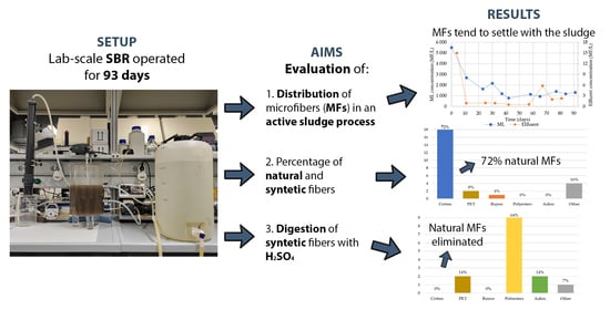
Assessment of Microplastics Distribution in a Biological Wastewater Treatment

by
Stefano Castelluccio
1,
Clara Bretas Alvim
2,
María Amparo Bes-Piá
2,
José Antonio Mendoza-Roca
2 and
Silvia Fiore
1,*
1
DIATI, Department of Engineering for Environment, Land, and Infrastructures, Politecnico di Torino, Corso Duca degli Abruzzi 24, 10129 Turin, Italy
2
Instituto de Seguridad Industrial, Radiofísica y Medioambiental, Universitat Politècnica de València, Camino de Vera, s/n, 46022 Valencia, Spain
*
Author to whom correspondence should be addressed.
Microplastics 2022, 1(1), 141-155; https://doi.org/10.3390/microplastics1010009
Submission received: 19 December 2021 / Revised: 19 January 2022 / Accepted: 28 January 2022 / Published: 1 February 2022

Abstract

:
Full-scale wastewater treatment facilities are not able to prevent microplastics (MPs) from discharging into natural waters and they are also associated with the land application of the sludge. This study evaluates the distribution of microfibers (MFs) in a lab-scale sequencing batch reactor (SBR) fed by synthetic wastewater (SW) for 93 days. The MFs were analyzed through optical microscopy in the mixed liquor (ML) and the effluent, and sulfuric acid digestion was applied to discriminate between natural and synthetic MFs (i.e., MPs). The results of the optical microscopy analyses were further validated through FTIR spectroscopy. A model describing the evolution over time of the MF concentration in the ML was created, accounting for the MFs entering the system through the SW and atmospheric deposition. The ratio between the MF concentration in the ML and the effluent was 1409 ± 781, demonstrating that MFs settle with the sludge. Consistently, in the ML, 64.9% of the recovered MFs were smaller than 1000 µm (average size 968 µm), while in the effluent, 76.1% of MFs were smaller than 1000 µm (average size 772 µm). Overall, 72% of MFs recovered from the ML were natural fibers and sulfuric acid digestion was successful in eliminating the natural MFs.

Graphical Abstract

1. Introduction

Although microplastics (MPs) are found in all types of habitats, from water to sediments and soil, in urban and remote areas [1], the highest concern has been raised regarding aquatic ecosystems [2,3]. Over the last decade, the focus on microplastics as emerging pollutants has seen a large increase on a global scale, resulting in a significant growth in the literature on the topic [3,4]. The main sources of MPs are the wear or breakdown of larger polymeric products, such as tires or artificial turf [5,6], the microfibers released from the washing of textiles [5,7], and the plastic particles used in manufacturing processes, such as air-blasting technology [1,8]. A recent study [7] estimated a release of 18 × 106 MP fibers for a household wash load of 6 kg of textiles made from synthetic fibers. Recent literature [9,10] has demonstrated that wastewater treatment plants (WWTPs) are not able to prevent the release of MPs into natural waters, where they could harm the aquatic fauna [9]. Moreover, the sorption of contaminants on the MPs’ surface may occur and they can become carriers of toxic contaminants, such as heavy metals, polycyclic aromatic hydrocarbons, and polychlorinated biphenyls [10,11,12]. MPs may also leach the plastics’ additives, which are contaminants of concern in many cases [13]. In detail, MPs escape from full-scale WWTPs in two ways: through the treated wastewater and through the sludge. Firstly, since WWTPs do not currently apply treatment technologies specifically designed for the removal of MPs [14], they can be released with the depurated effluent. The measured removal rate of MPs in actual WWTPs is above 88%, and exceeds 97% when tertiary treatments are applied [1,9]. The second release pathway of MPs is represented by the sludge [15], of which 50% is disposed by land application in Europe and North America. Recently, a positive correlation between the amount of MPs in soil samples and sludge application has been observed [16,17,18] and the low mobilization of MPs toward deeper soil and drainage systems has been described [17,19].
According to a recent review paper [20], MPs were detected in WWTP influents ranging from 0.28 to 3.14 × 10⁴ particles/L; in WWTP effluents from 0.01 to 2.97 × 10² particles/L; and in sewage sludge from 4.40 × 10³ to 2.40 × 10⁵ particles/kg [20]. The reported MP concentrations and removal efficiencies derive from individual samples or meta-analyses [20], which means that a direct comparison is difficult. The discrepancies in the MP concentrations reported in different studies can be attributed partly to different levels of industrialization in the served areas, differences in WWTP size and process outline, and seasonal changes, but mostly to the application of different sampling and detection methods [9]. A harmonization of the MP detection methods is therefore urgently needed to critically analyze the results of different studies. Although a chemical characterization (e.g., through Fourier transform infrared (FTIR) or Raman spectroscopy techniques) would be preferable, the identification of MPs is often performed visually by optical microscopy [21]. Due to its time and financial requirements, chemical characterization is generally adopted to assist and confirm the visual identification of MPs [22]. To distinguish between natural and synthetic particles that have micrometric dimensions, criteria based on the physical and optical properties of the particles have been established [23,24]. However, numerous studies have reported that up to 90% of the particles that were visually identified as synthetic actually revealed a natural origin when chemically analyzed [25,26,27,28]. To our knowledge, an analytical protocol that can distinguish between natural and synthetic particles easily and reliably has not yet been developed. The application of dyes, such as rose bengal and Nile red, could help with the visual identification of MPs [27,29], but unsatisfactory results have been reported. Moreover, several open challenges, such as the need for a thorough digestion step to eliminate the natural particles, and their staining have been described [30,31,32]. Among WWT technologies, active sludge processes are of special interest since they may be assumed to be the most common technology applied to WWT. To our knowledge, two bottlenecks in the existing literature on MPs may be pointed out as follows. Firstly, there is a lack of studies that analyze the distribution of MPs in the outflows of WWTPs in a controlled environment and for an extended time. Secondly, there is a need to improve the visual identification of MPs to ease the time and economic costs related to the monitoring of the removal of MPs in full-scale WWTPs. In the given framework, the novelty of this study relies on the attempt to pay attention to the two above-mentioned knowledge gaps. Regarding the first knowledge gap, our research aimed to assess the distribution of MPs in a laboratory-scale sequencing batch reactor (SBR) seeded with waste activated sludge (WAS) and fed with synthetic wastewater (SW), which was operated for 93 days. The SBR was fed with SW to eliminate the qualitative variabilities that are intrinsic to full-scale WWTPs influents in terms of MP concentration and characteristics [33]. The SBR performances were monitored by analyzing the mixed liquor (ML) and the effluent to evaluate the variation of microfiber (MF) concentration over three months of operation. This study was focused on MFs, i.e., long fibrous material that has a length substantially longer than its width [34], and they were visually analyzed through optical microscopy. MPs may have different shapes [1], such as fiber, fragment, pellet, film, etc. In most studies, MFs account for over 65% of the total MPs [1]; specifically considering WWTPs influents, where MFs ranged from 53% to 57% of the total MPs [9]. Concerning the second knowledge gap, a sulfuric acid digestion protocol developed for the analysis of textile fibers [35] was adapted as a pretreatment to remove natural fibers from the samples that were analyzed visually and, therefore, to selectively detect the MPs among the MFs. The results of the optical microscopy analyses were further validated through FTIR spectroscopy.

2. Materials and Methods

2.1. Wastewater and Activated Sludge

The synthetic wastewater (SW) was prepared according to a previous study [36] with peptone, meat extract, and K2HPO4 diluted in tap water to achieve a chemical oxygen demand (COD) equal to 500 mg/L, a total nitrogen concentration 60 mg/L, and a total phosphorus concentration 5 mg/L. The SW provided a controlled inflow of MFs; the concentration measured in the tap water was 11.4 MFs/L after filtration through a fiberglass filter with a pore size of 1 µm. This value was in line with the findings of a recent study [37], which found MF concentrations in tap water varying from “non-detected” up to around 168 MFs/L.
Waste activated sludge (WAS) (total solids 4.9 g/L) was collected from a WWTP near Valencia (Spain) at the beginning of the experimental phase. The process outline of the WWTP involved preliminary, primary, secondary, and tertiary treatments. The WAS was diluted 1:1 v/v with tap water to seed the experimental setup.

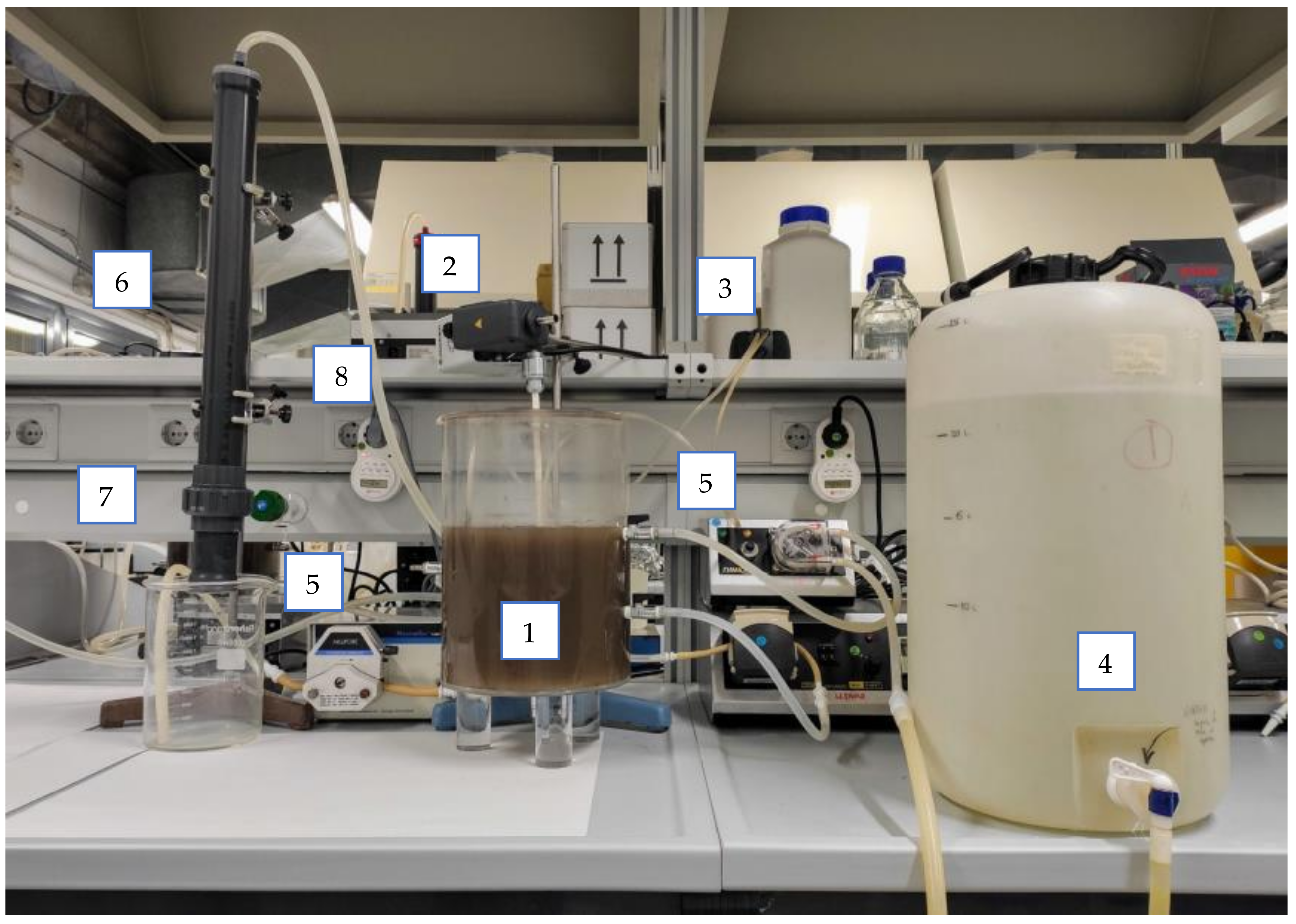
2.2. Experimental Setup

A laboratory-scale SBR was seeded with 2 L of diluted WAS and fed with 2 L of SW. The experimental setup (Figure 1) consisted of a 10 L (working volume 6 L) SBR equipped with a Heidolph RZR 1 stirrer and an air diffuser connected to an air pump. The SW was fed into the SBR from a 25 L tank through a peristaltic pump. A second peristaltic pump drew off the effluent into the effluent sampling device (ESD) made of a 6 × 50 cm PVC tube (see (6) in Figure 1). The effluent, entering from the top of the tube, was filtered at the bottom through a removable metallic sieve (mesh size 150 µm).
The SBR was operated for 93 days, applying 8 h cycles divided into three phases that were controlled by a timer: (1st) feeding of 2 L of SW, aeration, and mixing (6 h); (2nd) settling (1 h and 30 min); (3rd) extraction of 2 L of effluent (30 min). The processing of the 2 L in the feeding and the extraction phases resulted in a hydraulic retention time equal to 1 day. The mixed liquor suspended solid (MLSS) concentration was maintained between 2.5 g/L and 3.0 g/L through periodical withdrawals of the ML.

2.3. SBR Performance Monitoring

The ML was analyzed three times per week for the MLSS concentration [38] and once per week for the ML volatile suspended solids (MLVSS) content [38] and the zeta potential (Malvern Zetasizer Zeta Nano ZS). To evaluate the growth of the microorganisms in the ML, the cumulative MLSS (MLSSc) trend was calculated through Equation (1):
MLSSc(d) = MLSS(d) + ∑d MLSSr,i
where ∑d MLSSr,i is the sum of the decreases in MLSS concentration due to the excess ML withdrawal from day zero of the SBR operation to day ‘d’. The growth of the microorganisms (EGM) was estimated by normalizing the MLSSc with the initial value as in Equation (2):
EGM (d) = MLSSc(d)/MLSSc(0)
The EGM weekly rate (EGMwr) was calculated during the whole SBR operation period through Equation (3):
EGMwr = (EGM1 − EGM2)/(d1 − d2) × 100
where d1 and d2 were roughly separated by 7 days.
The effluent was analyzed three times per week for pH, electric conductivity (EC) (Crison GLP 31+ conductimeter), turbidity (Dinko D-112 turbidimeter), and COD (Spectroquant test kits and Merck Nova 30 photometer), and once per week for total nitrogen, NH4+, NO2, NO3, total phosphorus, PO43− (Spectroquant test kits and Merck Nova 30 photometer), and total organic carbon (TOC) (Shimadzu TOC analyzer TOC-LCPH/CPN).

2.4. Microfiber Analyses

The concentrations of MFs in the effluent and ML were monitored once per week. For the analysis of the effluent, the MFs were collected through the ESD. The 150 µm screen was removed from the casing and the retained material was transferred into a glass beaker. For the analysis of the ML, 100 mL were collected in a glass beaker. All samples underwent pretreatments with hydrogen peroxide to reduce their organic matter content. In detail, H2O2 (35%) was added to the effluent (1% v/v) and to the ML (50% v/v) [33]. The beaker containing the sample was then sealed, stirred, and heated at 60 °C for 120 min to obtain the digestion of the organic matter [39,40]. Only the digested ML samples (see Section 2.4.1) were then filtered through a 150 µm metallic sieve, reproducing the sampling conditions of the effluent to achieve consistency. To recover the MFs, the digested samples were finally vacuum filtered through a 1 µm pore size fiberglass filter.

2.4.1. Sulfuric Acid Digestion Protocol

The digestion protocol developed by the American Association of Textile Chemists and Colorists (AATCC) [35] was adapted to MF characterization. The filter with the recovered particles was managed in two alternate ways. In one way, it was placed on a Büchner flask that was connected to a vacuum pump. In the second way, the filter was inserted into a glass funnel placed over a Büchner flask that was connected to a vacuum pump. In both cases, 100 mL of H2SO4 (70%) was carefully poured into the filter and after 15 min, the vacuum pump was turned on to drain the excess liquor. The filter was then vacuum washed, first with 50 mL of H2SO4 (5%) and then with distilled water until the filtrate reached neutrality. The pump was turned off and 25 mL of NH4OH (8%) was poured into the funnel. After 10 min, the excess liquor was vacuum drained. The filter was washed again with 150 mL of distilled water, removed from the funnel, and dried.

2.4.2. Physical Characterization

The pretreated samples were visually analyzed with a Leica MZ APO stereomicroscope. The filters were divided into eight sequentially enumerated portions using a grid [41] to lower the probability of duplicated or missed counts [9]. The analyzed parameters were the number of recovered MFs and their size and color. Considering the mesh size of the filters adopted to collect/pretreat the samples, only MFs longer than 150 µm were counted. The following criteria were applied to distinguish the MPs from the natural fibers: no visible cellular or organic structures; fibers equally thick throughout their entire length; and clear and homogeneous colors [23,24]. The 150 µm–5000 µm dimensional range was divided into 50 µm intervals, and for each interval the number of recovered MFs was counted. The size distribution of the recovered MFs was estimated using the data obtained from all samples and characterized by the probability mass function (PMF) and the cumulative distribution function (CDF) [42].

2.4.3. Chemical Characterization

The chemical characterization of the MFs was performed to assess the percentage of MPs and the relative abundance of different polymer types. The MFs were identified as MPs through an FTIR spectrometer Bruker Vertex 80 coupled with a Bruker Hyperion 1000 microscope operated in ATR mode. The collected spectra were corrected using the Bruker Opus and the KnowItAll software [43] and then compared to the built-in reference spectra library and the spectra library of textile fibers developed by the Institute of Chemistry, University of Tartu [44]. The recommended identification protocols [43,44] were applied.

2.4.4. Microfiber Distribution Model

A model describing the evolution over time of the MF concentration in the ML was created. The model was based on the mass balance of the MFs in the SBR system. The initial amount of MFs was calculated by multiplying the initial MF concentration of the ML by the reactor volume. For each day, the MFs entering the system due to atmospheric deposition were considered and the MFs that were removed were subtracted.
Then, the modeled MF concentration was calculated by dividing the estimated total number of MFs by the reactor volume. The same process was repeated for every day of the experiment. The MFs entering the SBR were divided into two contributions: the MFs present in the simulated wastewater and the MFs entering from a circular opening on top of the SBR due to atmospheric deposition. The two contributions were calculated through Equations (4) and (5):
FEEDin = Ctw × Vfeed
where FEEDin is the number of MFs entering the system with the SW, Ctw is the concentration of MFs in the tap water that was measured using the ESD, and Vfeed is the volume of SW;
ATMDin = Fdep × Aop
where ATMDin is the number of MFs entering the system through atmospheric deposition, Fdep is the daily flux of deposited MFs, and Aop is the area of the circular opening on top of the SBR.
The MFs leaving the system were also divided into two contributions: the MFs present in the SBR effluent and the MFs contained in the excess ML that was removed. The 2 contributions were calculated through Equations (6) and (7):
EFFLout = Ceffl × Veffl
where EFFLout is the number of MFs in the effluent, Ceffl is the concentration of MFs in the effluent, and Veffl is the volume of effluent;
EXCSout = Cmixl ·× Vmixl
where EXCSout is the number of MFs in the excess ML that was removed, Cmixl is the concentration of MFs in the ML, and Vmixl is the volume of excess ML that was removed. Biodegradation was not considered since it occurs at slow rates [45] compared to the duration of our research.

2.5. Quality Assurance and Quality Control

To limit any contamination of the samples, specific guidelines were followed. All equipment was thoroughly rinsed and working surfaces were cleaned with ethanol [9,30]. Plastic equipment was replaced by glass and metal counterparts, when possible, and laboratory coats made from cotton were used [31] and synthetic clothes were avoided. Any contact between the surfaces of the plastic equipment that was used (Figure 1 (1,4)) and abrasive material was avoided to limit any possible contamination. The whole experimental setup was closed or covered with aluminum foil. All samples were sealed in clean Petri dishes or covered with aluminum foil [9,31]. During the physical characterization, the grid used to divide the filter into portions also avoided the airborne contamination of the samples. The concentration of MFs in the tap water that was used to prepare the SW was measured by filtering 5 L of tap water through a 1 µm fiberglass filter. Then, 50 L of tap water went through the effluent sampling device to estimate the MF recovery. Atmospheric deposition Fdep was assessed by placing a 1 µm fiberglass filter on the workspace in an open Petri dish for 1 week.

3. Results and Discussions

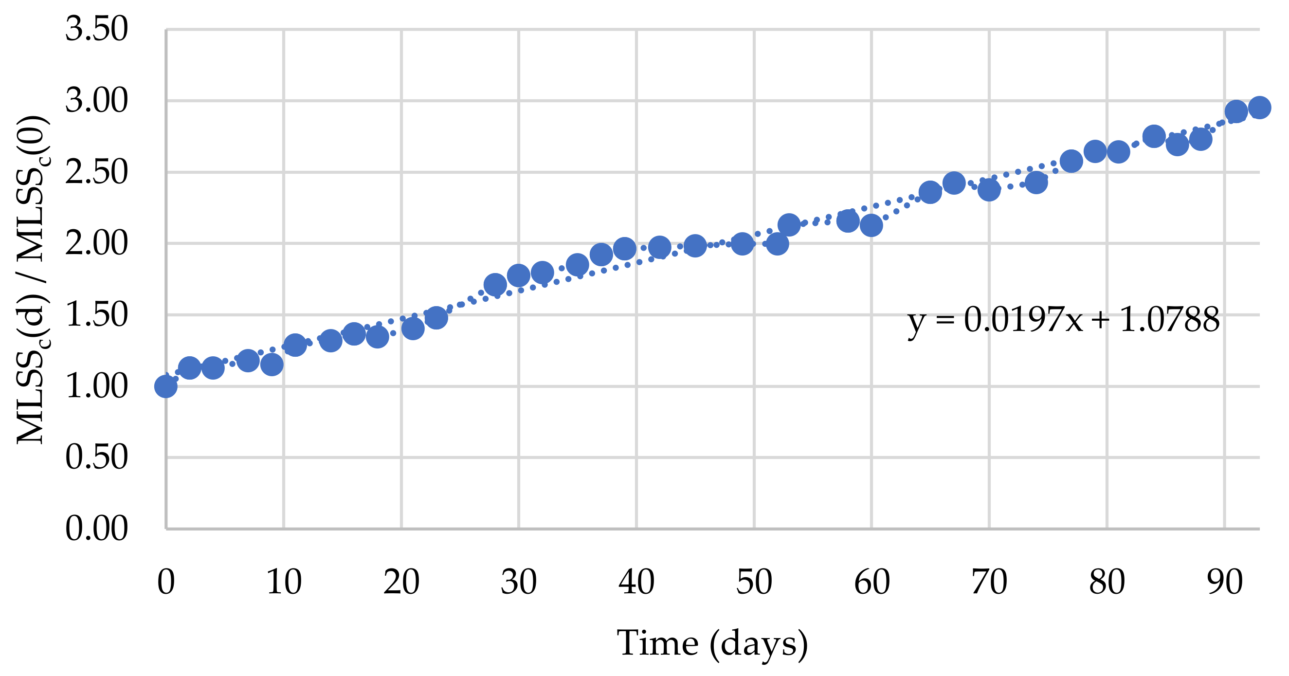
3.1. SBR Performance Monitoring

The average physicochemical features of the SBR effluent that was measured over 93 days (Table 1) showed relatively stable parameters. The observed removals (average values measured over the test period) were 96.35 ± 1.56% for the COD and 25.6 ± 12.4% for the total nitrogen, while the removal of total phosphorus was not observed.
The EGM trend (Figure 2) showed that the growth of the microorganisms in the ML was steady throughout the SBR operation, with an average EGMwr equal to 14.7%. The average MLVSS content was 89.2 ± 4.2%, in line with typical MLVSS/MLSS ratios [46] and the average z potential was −10.76 ± 1.13 mV.

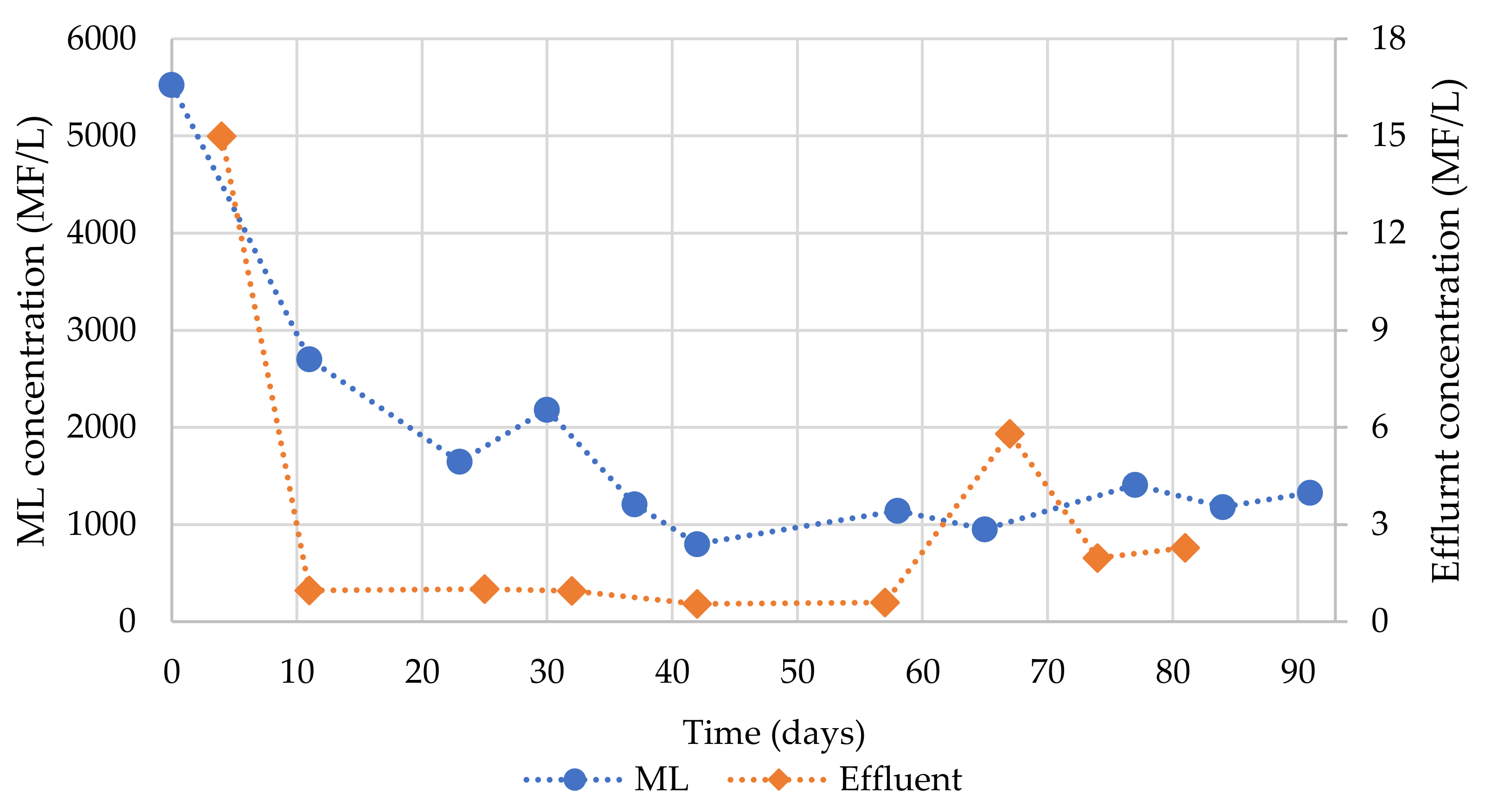
3.2. Microfiber Analyses

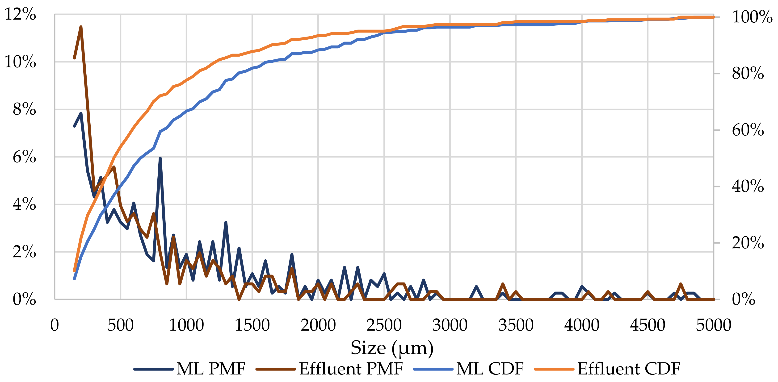
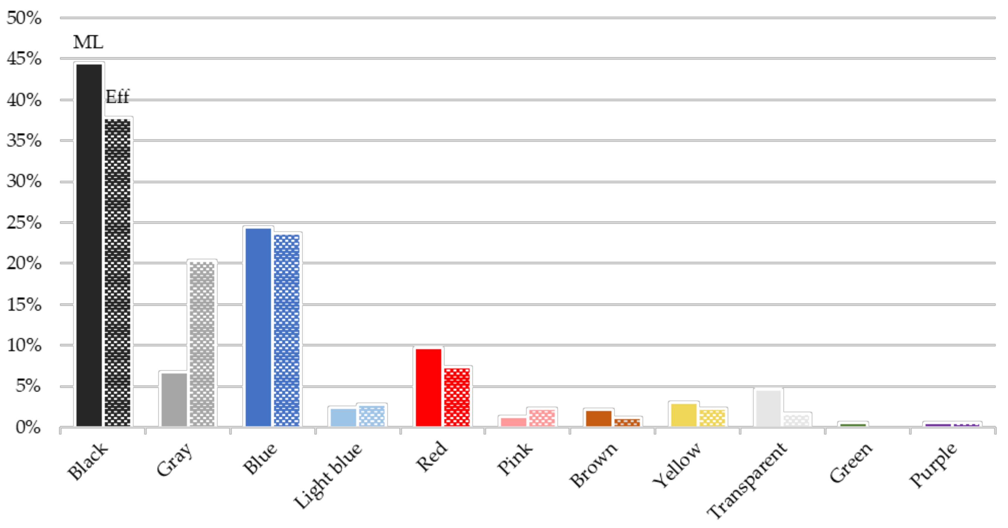
3.2.1. Physical Characterization

MF concentration in the ML and in the effluent decreased with time (Figure 3), as expected. Before the tests, the WAS was exposed to the inflow of a full-scale WWTP and contained a much higher concentration of MPs compared to the SW. According to some references, WAS has the capacity to remove some of the MPs from the influent and retain them [41,47]. The observed decrease in MF concentration in the ML demonstrates that MPs exit the system through the sludge withdrawal. MF concentration in the ML showed a clear decrease (from 5525 MFs/L to 800 MFs/L) in the first 40 days (Figure 3). The rate of the decrease diminished with time and after 40 days, the concentration of MFs in the ML remained stable in the 800 to 1410 MFs/L range. On the other hand, MF concentration in the SBR effluent showed a rapid decrease (from 14.99 MFs/L to 0.96 MFs/L) in the first 10 days of the experiment (Figure 3). After the first 10 days, the MF concentration in the effluent was relatively stable, ranging from 0.55 MFs/L to 2.28 MFs/L. However, for the effluent filtered between 64 and 70 days after the start of the experiment, a concentration of 5.81 MFs/L was measured. Various factors could have caused this anomalous spike: errors during the collection or pretreatment processes; a spike in the MF concentration in the tap water that was used to prepare the SW, which would also explain the slight increase in MFs in the ML sample; or the relatively low amount of water filtered through the ESD during that period, which led to a lower representativeness of that specific sample. The previously described factors are not mutually exclusive and could have all contributed to the observed result. Figure 3 also highlights the presence of a horizontal asymptote for both ML and effluent MF concentration, suggesting that an equilibrium between the MFs entering and leaving the SBR was reached in the later stage of the experiment.
The relatively slow decrease in MF concentration in the ML suggested that the MFs have a strong tendency to be retained by the sludge during settling. This consideration was supported by the persistence of the difference in MF concentration in the later stages of the experiment and by previous studies [41,48,49]. The average ratio between the MF concentration in the ML and in the effluent was 1409 ± 781 and, although a clear decrease over time can be noticed, the MF concentration in the ML was always at least two orders of magnitude greater than the concentration in the effluent.
The concentration of MFs measured in tap water was 2.3 MFs/L when it was filtered through the ESD, which allowed us to estimate a 20% MF recovery rate for the ESD. The recovery rate was relatively low because fibers longer than the mesh size could pass longitudinally through the sieve [9,30]. The calculated atmospheric deposition was 247 MFs/m2·day.
In the ML, 64.9% of the recovered MFs were smaller than 1000 µm (average size 968 µm), while in the effluent, 76.1% of the MFs were smaller than 1000 µm (average size 772 µm) (Figure 4). The higher proportion of small fibers in the effluent compared to the ML confirmed the results of previous studies [50] and supported the evidence that larger MFs are more likely to be sequestrated by the sludge and removed during the settling phase.
The color distributions of the MFs in the ML and in the effluent are similar (Figure 5). The biggest challenge encountered during the definition of the MF color distribution was detecting particles with a color similar to the background [50], which was white in this research. Most studies showed a higher proportion of white MFs, which often accounted for the majority of the recovered MFs [25,51]. The problem may have been exacerbated by the use of hydrogen peroxide during the pretreatment phase, which can cause discoloration in MFs [31]. Particles with eye-catching colors have a higher probability of being selected for the chemical identification whereas those with dull colors are easily overlooked, thus potentially introducing bias [25,52]. However, the association between MPs’ color and specific polymer types has been described as unlikely [25], which decreases the probability of color-based bias during chemical identification.

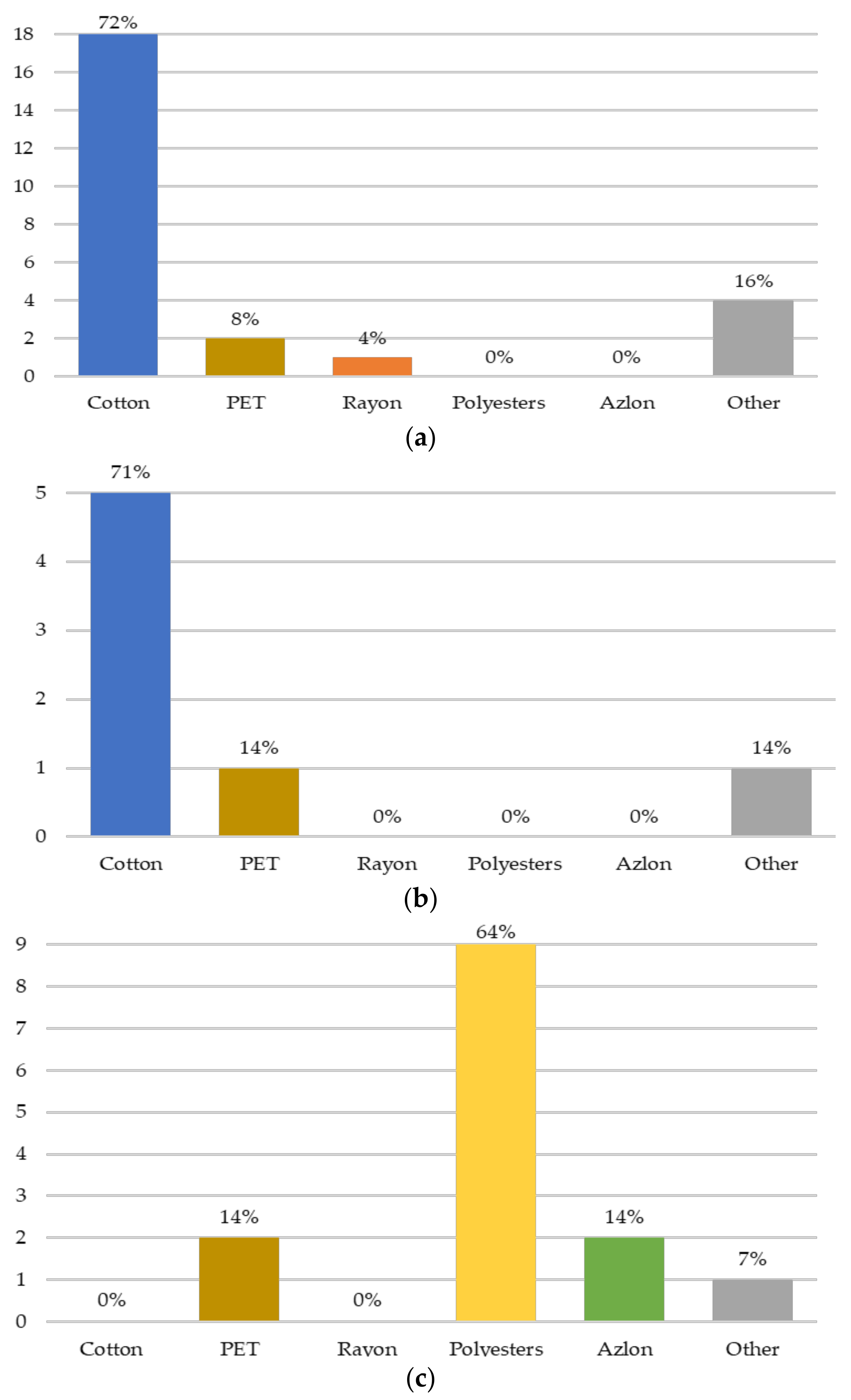
3.2.2. Chemical Characterization

In total, 25 MFs were recovered from the ML that was collected on day 1 of the experiment; this sample was not digested with sulfuric acid. Figure 6a highlights that 72% of the MFs recovered from the initial ML sample were natural fibers, in agreement with other studies [25,26,27,28] and confirming the need for the definition of a reliable procedure to visually distinguish between natural and synthetic MFs. Of the analyzed fibers, 18 were identified as cotton, 2 as PET, 1 as rayon, and 4 were unidentified (Figure 6a).
Of the seven MFs that were recovered from the ML sample collected on day 77, five were identified as cotton fibers, one as PET fiber, and one was unidentified (Figure 6b). The first adaptation of the digestion protocol (i.e., the filter directly placed on the Büchner) was unsuccessful, as cotton fibers still accounted for 71% of the MFs.
Afterward, the same ML sample that was collected on day 1 underwent the second adaptation of the digestion protocol (i.e., the filter placed in a glass funnel connected to the Büchner). Of the 14 collected MFs, 9 were identified as polyester, 2 as PET, 2 as Azlon, and 1 was unidentified (Figure 6c). The application of the second adaptation of the protocol was successful in eliminating the natural MFs, as their proportion in the same sample decreased from 72% to “non-detected”.
Some examples of the gathered FTIR spectra are shown in Figure 7.

3.3. MF Distribution Model

The modeled MF concentration in the ML is plotted against the measured MF concentration in Figure 8. Both trends decreased, although the modeled curve decreased at a slower rate initially. Additionally, the modeled curve did not have a horizontal asymptote in the later stage of the experiment. Both differences can be partly explained by the low recovery rate of MFs in the effluent; the low recovery rate underestimated the actual concentration of MFs EFFLout leaving the SBR with the effluent, which could explain the initial slow decrease rate in the modeled MF concentration in the ML. The effluent concentration was not corrected accounting for the recovery rate of the ESD because that value was not representative of the whole collection process of the SBR effluent. The recovery rate of the ESD was measured by filtering tap water continuously. On the contrary, the effluent was sampled discontinuously for 1 week. The discontinuity of the process might favor the rearrangement of the fibers captured by the removable sieve, which could increase the portion of MFs that passed longitudinally through the sieve. To maintain consistency between the adopted protocols, the MF concentration in the tap water used in the model was the same value measured with the ESD (see Section 2.5). This choice, although improving uniformity, underestimated the number of MFs FEEDin entering in the system with the SW. The underestimation of FEEDin could explain why the positive and negative contributions were not balanced in the model in the later stage of the experiment and why the modeled curve did not have the horizontal asymptote shown by the measured data. To improve the fit of the model, further refinements are needed. Firstly, the quantification of the exact recovery rate of the effluent collection phase, as well as the recovery rate of the ML collection phase, are needed. Then, it is advised that the eventual variations over time of MF concentration in the tap water be monitored.

4. Conclusions

This research attempted to address two key issues related to the study of the presence of microplastics (MPs) within wastewater treatment processes. In the considered experimental conditions that focused on the study on microfiber (MF) distribution and the identification of their synthetic fraction (i.e., fiber MPs), the following statements can be made.
Distribution of MFs in a lab-scale activated sludge process: The analysis of the MFs in the mixed liquor (ML) showed a clear decrease in the first 40 days of the experiment (from 5525 to 800 MFs/L), which was mainly due to the sludge withdrawal since the synthetic wastewater contained a lower concentration of MFs compared to a real WWTP influent. Additionally, the relatively slow concentration decrease in the ML, paired with a difference of at least two orders of magnitude between the concentrations detected in the ML and in the effluent, suggested that MFs have a strong tendency to settle with the sludge. This was consistent with the fact that the effluent displayed a higher proportion of smaller fibers compared to the ML. The modeled ML concentration was able to reproduce the decreasing trend in MF concentration, although not fully reliably. To improve the fit of the model, further refinements are needed: the quantification of the exact recovery rate of the effluent and of the ML and the monitoring of the eventual variations of MF concentration in the inflow (SW was based on tap water).
Percentage of synthetic fibers (i.e., fiber MPs) among the collected MFs: According to the chemical characterization, 72% of the recovered MFs from the ML were natural fibers, underlining the need for a reliable procedure to visually identify synthetic microfibers. The second adaptation of the sulfuric digestion protocol was successful in eliminating natural fibers. Even though the results of the herein presented preliminary tests were promising, further studies are needed to better understand the effect of the adapted digestion protocol on synthetic MFs, with particular attention on nylon, rayon, and spandex, which are soluble or partially soluble in sulfuric acid.

Author Contributions

Conceptualization and methodology, M.A.B.-P., J.A.M.-R., and S.F.; supervision, C.B.A., M.A.B.-P., J.A.M.-R., and S.F.; validation, S.C.; investigation, data curation, and visualization, S.C.; writing—original draft preparation, S.C.; writing—review and editing, all authors. All authors have read and agreed to the published version of the manuscript.

Funding

This research was funded by the Spanish Ministry of Science, Innovation and Universities (grant number: RTI2018-096916-B-I00).

Institutional Review Board Statement

Not applicable.

Informed Consent Statement

Not applicable.

Data Availability Statement

Data is contained within the article.

Conflicts of Interest

The authors declare no conflict of interest.

References

  1. Ngo, P.L.; Pramanik, B.K.; Shah, K.; Roychand, R. Pathway, classification and removal efficiency of microplastics in wastewater treatment plants. Environ. Pollut. 2019, 255, 113326. [Google Scholar] [CrossRef] [PubMed]
  2. Vivekanand, A.C.; Mohapatra, S.; Tyagi, V.K. Microplastics in aquatic environment: Challenges and perspectives. Chemosphere 2021, 282, 131151. [Google Scholar] [CrossRef] [PubMed]
  3. Liu, S.; Huang, J.; Zhang, W.; Shi, L.; Yi, K.; Yu, H.; Zhang, C.; Li, S.; Li, J. Microplastics as a vehicle of heavy metals in aquatic environments: A review of adsorption factors, mechanisms, and biological effects. J. Environ. Manag. 2021, 302, 113995. [Google Scholar] [CrossRef] [PubMed]
  4. Frias, J.P.G.L.; Nash, R. Microplastics: Finding a consensus on the definition. Mar. Pollut. Bull. 2019, 138, 145–147. [Google Scholar] [CrossRef]
  5. Wang, T.; Li, B.; Yu, W.; Zou, X. Microplastic pollution and quantitative source apportionment in the Jiangsu coastal area, China. Mar. Pollut. Bull. 2021, 166, 112237. [Google Scholar] [CrossRef]
  6. Luo, Z.; Zhou, X.; Su, Y.; Wang, H.; Yu, R.; Zhou, S.; Xu, E.G.; Xing, B. Environmental occurrence, fate, impact, and potential solution of tire microplastics: Similarities and differences with tire wear particles. Sci. Total Environ. 2021, 795, 148902. [Google Scholar] [CrossRef]
  7. Galvão, A.; Aleixo, M.; De Pablo, H.; Lopes, C.; Raimundo, J. Microplastics in wastewater: Microfiber emissions from common household laundry. Environ. Sci. Pollut. Res. 2020, 27, 26643–26649. [Google Scholar] [CrossRef]
  8. Kurniawan, S.B.; Said, N.S.M.; Imron, M.F.; Abdullah, S.R.S. Microplastic pollution in the environment: Insights into emerging sources and potential threats. Environ. Technol. Innov. 2021, 23, 101790. [Google Scholar] [CrossRef]
  9. Sun, J.; Dai, X.; Wang, Q.; van Loosdrecht, M.C.; Ni, B.-J. Microplastics in wastewater treatment plants: Detection, occurrence and removal. Water Res. 2019, 152, 21–37. [Google Scholar] [CrossRef]
  10. Li, X.; Mei, Q.; Chen, L.; Zhang, H.; Dong, B.; Dai, X.; He, C.; Zhou, J. Enhancement in adsorption potential of microplastics in sewage sludge for metal pollutants after the wastewater treatment process. Water Res. 2019, 157, 228–237. [Google Scholar] [CrossRef]
  11. Avio, C.G.; Gorbi, S.; Milan, M.; Benedetti, M.; Fattorini, D.; D’Errico, G.; Pauletto, M.; Bargelloni, L.; Regoli, F. Pollutants bioavailability and toxicological risk from microplastics to marine mussels. Environ. Pollut. 2015, 198, 211–222. [Google Scholar] [CrossRef]
  12. Carbery, M.; O’Connor, W.; Palanisami, T. Trophic transfer of microplastics and mixed contaminants in the marine food web and implications for human health. Environ. Int. 2018, 115, 400–409. [Google Scholar] [CrossRef] [Green Version]
  13. Hermabessiere, L.; Dehaut, A.; Paul-Pont, I.; Lacroix, C.; Jezequel, R.; Soudant, P.; Duflos, G. Occurrence and effects of plastic additives on marine environments and organisms: A review. Chemosphere 2017, 182, 781–793. [Google Scholar] [CrossRef] [Green Version]
  14. Ou, H.; Zeng, E.Y. Chapter 10—Occurrence and Fate of Microplastics in Wastewater Treatment Plants. In Microplastic Contamination in Aquatic Environments; Zeng, E.Y., Ed.; Elsevier: Amsterdam, The Netherlands, 2018; pp. 317–338. [Google Scholar]
  15. Sol, D.; Laca, A.; Laca, A.; Díaz, M. Approaching the environmental problem of microplastics: Importance of WWTP treatments. Sci. Total Environ. 2020, 740, 140016. [Google Scholar] [CrossRef]
  16. Corradini, F.; Meza, P.; Eguiluz, R.; Casado, F.; Huerta-Lwanga, E.; Geissen, V. Evidence of microplastic accumulation in agricultural soils from sewage sludge disposal. Sci. Total Environ. 2019, 671, 411–420. [Google Scholar] [CrossRef]
  17. Schell, T.; Hurley, R.; Buenaventura, N.T.; Mauri, P.V.; Nizzetto, L.; Rico, A.; Vighi, M. Fate of microplastics in agricultural soils amended with sewage sludge: Is surface water runoff a relevant environmental pathway? Environ. Pollut. 2021, 293, 118520. [Google Scholar] [CrossRef]
  18. van Den Berg, P.; Huerta-Lwanga, E.; Corradini, F.; Geissen, V. Sewage sludge application as a vehicle for microplastics in eastern Spanish agricultural soils. Environ. Pollut. 2020, 261, 114198. [Google Scholar] [CrossRef]
  19. Tagg, A.S.; Brandes, E.; Fischer, F.; Fischer, D.; Brandt, J.; Labrenz, M. Agricultural application of microplastic-rich sewage sludge leads to further uncontrolled contamination. Sci. Total Environ. 2021, 806, 150611. [Google Scholar] [CrossRef]
  20. Liu, W.; Zhang, J.; Liu, H.; Guo, X.; Zhang, X.; Yao, X.; Cao, Z.; Zhang, T. A review of the removal of microplastics in global wastewater treatment plants: Characteristics and mechanisms. Environ. Int. 2021, 146, 106277. [Google Scholar] [CrossRef]
  21. Tirkey, A.; Upadhyay, L.S.B. Microplastics: An overview on separation, identification and characterization of microplastics. Mar. Pollut. Bull. 2021, 170, 112604. [Google Scholar] [CrossRef]
  22. Institute for Environment and Sustainability (Joint Research Centre), MSFD Technical Subgroup on Marine Litter. Guidance on Monitoring of Marine Litter in European Seas; Publications Office of the European Union: Luxembourg, 2013. [Google Scholar]
  23. Riani, E.; Cordova, M.R. Microplastic ingestion by the sandfish Holothuria scabra in Lampung and Sumbawa, Indonesia. Mar. Pollut. Bull. 2021, 2021, 113134. [Google Scholar] [CrossRef]
  24. Suteja, Y.; Atmadipoera, A.S.; Riani, E.; Nurjaya, I.W.; Nugroho, D.; Cordova, M.R. Spatial and temporal distribution of microplastic in surface water of tropical estuary: Case study in Benoa Bay, Bali, Indonesia. Mar. Pollut. Bull. 2021, 163, 111979. [Google Scholar] [CrossRef]
  25. Hidalgo-Ruz, V.; Gutow, L.; Thompson, R.C.; Thiel, M. Microplastics in the Marine Environment: A Review of the Methods Used for Identification and Quantification. Environ. Sci. Technol. 2012, 46, 3060–3075. [Google Scholar] [CrossRef]
  26. Gies, E.A.; LeNoble, J.L.; Noël, M.; Etemadifar, A.; Bishay, F.; Hall, E.R.; Ross, P.S. Retention of microplastics in a major secondary wastewater treatment plant in Vancouver, Canada. Mar. Pollut. Bull. 2018, 133, 553–561. [Google Scholar] [CrossRef]
  27. Ziajahromi, S.; Neale, P.A.; Rintoul, L.; Leusch, F.D.L. Wastewater treatment plants as a pathway for microplastics: Development of a new approach to sample wastewater-based microplastics. Water Res. 2017, 112, 93–99. [Google Scholar] [CrossRef]
  28. Yang, L.; Li, K.; Cui, S.; Kang, Y.; An, L.; Lei, K. Removal of microplastics in municipal sewage from China’s largest water reclamation plant. Water Res. 2019, 155, 175–181. [Google Scholar] [CrossRef]
  29. Prata, J.C.; Reis, V.; Matos, J.T.; da Costa, J.P.; Duarte, A.C.; Rocha-Santos, T. A new approach for routine quantification of microplastics using Nile Red and automated software (MP-VAT). Sci. Total Environ. 2019, 690, 1277–1283. [Google Scholar] [CrossRef]
  30. Alvim, C.B.; Mendoza-Roca, J.-A.; Bes-Piá, A. Wastewater treatment plant as microplastics release source—Quantification and identification techniques. J. Environ. Manag. 2020, 255, 109739. [Google Scholar] [CrossRef]
  31. Prata, J.C.; da Costa, J.P.; Duarte, A.C.; Rocha-Santos, T. Methods for sampling and detection of microplastics in water and sediment: A critical review. TrAC Trends Anal. Chem. 2019, 110, 150–159. [Google Scholar] [CrossRef]
  32. Shim, W.J.; Hong, S.H.; Eo, S.E. Identification methods in microplastic analysis: A review. Anal. Methods 2017, 9, 1384–1391. [Google Scholar] [CrossRef]
  33. Alvim, C.B.; Castelluccio, S.; Ferrer-Polonio, E.; Bes-Piá, M.; Mendoza-Roca, J.; Fernández-Navarro, J.; Alonso, J.; Amorós, I. Effect of polyethylene microplastics on activated sludge process—Accumulation in the sludge and influence on the process and on biomass characteristics. Process Saf. Environ. Prot. 2021, 148, 536–547. [Google Scholar] [CrossRef]
  34. GESAMP. Guidelines or the Monitoring and Assessment of Plastic Litter and Microplastics in the Ocean; GESAMP Joint Group of Experts on the Scientific Aspects of Marine Environmental Protection: London, UK, 2019; 130p. [Google Scholar]
  35. American Association of Textile Chemists and Colorists (AATCC). AATCC 20A: Test Method for Fiber Analysis: Quantitative 2020; American Association of Textile Chemists and Colorists (AATCC): Durham, NC, USA, 2021. [Google Scholar]
  36. Ferrer-Polonio, E.; White, K.; Mendoza-Roca, J.-A.; Bes-Piá, A. The role of the operating parameters of SBR systems on the SMP production and on membrane fouling reduction. J. Environ. Manag. 2018, 228, 205–212. [Google Scholar] [CrossRef] [PubMed]
  37. Sol, D.; Laca, A.; Laca, A.; Díaz, M. Microplastics in Wastewater and Drinking Water Treatment Plants: Occurrence and Removal of Microfibres. Appl. Sci. 2021, 11, 10109. [Google Scholar] [CrossRef]
  38. American Public Health Association (APHA); American Water Works Association (AWWA); Water Environment Federation (WEF). Standard Methods for the Examination of Water and Wastewater, 22nd ed.; APHA: Washington, DC, USA, 2012. [Google Scholar]
  39. Avio, C.G.; Gorbi, S.; Regoli, F. Experimental development of a new protocol for extraction and characterization of microplastics in fish tissues: First observations in commercial species from Adriatic Sea. Mar. Environ. Res. 2015, 111, 18–26. [Google Scholar] [CrossRef]
  40. Cole, M.; Webb, H.; Lindeque, P.K.; Fileman, E.S.; Halsband, C.; Galloway, T.S. Isolation of microplastics in biota-rich seawater samples and marine organisms. Sci. Rep. 2014, 4, 4528. [Google Scholar] [CrossRef] [Green Version]
  41. Carr, S.A.; Liu, J.; Tesoro, A.G. Transport and fate of microplastic particles in wastewater treatment plants. Water Res. 2016, 91, 174–182. [Google Scholar] [CrossRef]
  42. DeCoursey, W. Chapter 5—Probability Distributions of Discrete Variables: For this chapter the reader should have a solid understanding of sections 2.1, 2.2, 3.1, and 3.2. In Statistics and Probability for Engineering Applications; DeCoursey, W.J., Ed.; Burlington: Newnes, Australia, 2003; pp. 84–140. [Google Scholar]
  43. Lasch, P. Spectral pre-processing for biomedical vibrational spectroscopy and microspectroscopic imaging. Chemom. Intell. Lab. Syst. 2012, 117, 100–114. [Google Scholar] [CrossRef] [Green Version]
  44. Institute of Chemistry University of Tartu. Textile Fibres—Database of ATR-FT-IR Spectra of Various Materials 2021. Available online: https://spectra.chem.ut.ee/textile-fibres/ (accessed on 10 December 2021).
  45. Ali, M.U.; Lin, S.; Yousaf, B.; Abbas, Q.; Munir, M.A.M.; Rasihd, A.; Zheng, C.; Kuang, X.; Wong, M.H. Environmental emission, fate and transformation of microplastics in biotic and abiotic compartments: Global status, recent advances and future perspectives. Sci. Total Environ. 2021, 791, 148422. [Google Scholar] [CrossRef]
  46. Metcalf & Eddy. Wastewater Engineering: Treatment and Reuse, 4th ed.; McGraw-Hill: New York, NY, USA, 2003. [Google Scholar]
  47. Lares, M.; Ncibi, M.C.; Sillanpää, M.; Sillanpää, M. Occurrence, identification and removal of microplastic particles and fibers in conventional activated sludge process and advanced MBR technology. Water Res. 2018, 133, 236–246. [Google Scholar] [CrossRef]
  48. Mahon, A.M.; O’Connell, B.; Healy, M.; O’Connor, I.; Officer, R.; Nash, R.; Morrison, L. Microplastics in Sewage Sludge: Effects of Treatment. Environ. Sci. Technol. 2017, 51, 810–818. [Google Scholar] [CrossRef]
  49. Liu, X.; Yuan, W.; Di, M.; Li, Z.; Wang, J. Transfer and fate of microplastics during the conventional activated sludge process in one wastewater treatment plant of China. Chem. Eng. J. 2019, 362, 176–182. [Google Scholar] [CrossRef]
  50. Murphy, F.; Ewins, C.; Carbonnier, F.; Quinn, B. Wastewater Treatment Works (WwTW) as a Source of Microplastics in the Aquatic Environment. Environ. Sci. Technol. 2016, 50, 5800–5808. [Google Scholar] [CrossRef] [Green Version]
  51. Li, X.; Chen, L.; Mei, Q.; Dong, B.; Dai, X.; Ding, G.; Zeng, E.Y. Microplastics in sewage sludge from the wastewater treatment plants in China. Water Res. 2018, 142, 75–85. [Google Scholar] [CrossRef]
  52. Nuelle, M.-T.; Dekiff, J.H.; Remy, D.; Fries, E. A new analytical approach for monitoring microplastics in marine sediments. Environ. Pollut. 2014, 184, 161–169. [Google Scholar] [CrossRef]
Figure 1. The outline of the experimental setup: (1) SBR (sequencing batch reactor); (2) stirrer; (3) air pump; (4) SW (synthetic wastewater) feed tank; (5) peristaltic pumps; (6) effluent sampling device; (7) removable screen; (8) timer outlet for the control of the sequencing phases in the SBR.
Microplastics 01 00009 g001
Figure 2. The estimated growth of the microorganisms in the mixed liquor during the test period (MLSS: mixed liquor suspended solids).
Microplastics 01 00009 g002
Figure 3. The trends of the microfiber (MF) concentration in the mixed liquor (ML) and in the effluent during the test period.
Microplastics 01 00009 g003
Figure 4. The trends of the probability mass function (PMF) and cumulative distribution function (CDF) of the sizes of the MFs recovered from the mixed liquor (ML) (dark and light blue) and from the effluent (dark and light orange).
Microplastics 01 00009 g004
Figure 5. The color distribution of the microfibers recovered from the mixed liquor (ML) (solid) and the effluent (gingham) samples.
Microplastics 01 00009 g005
Figure 6. The composition of the microfibers in the analyzed samples: (a) day 1, mixed liquor (ML), no digestion; (b) day 77, ML after the first adaptation of the digestion protocol; (c) day 1, ML after the second adaptation of the digestion protocol.
Microplastics 01 00009 g006
Figure 7. The FTIR spectra of the microfibers compared to the reference spectra: (a) a cotton fiber from the mixed liquor (ML) on day 1 (undigested); (b) a PET fiber from the ML on day 1 (undigested); (c) a polyester fiber from the ML digested on day 1 (second adaptation of the protocol); (d) a PET fiber from the ML digested on day 1 (second adaptation of the protocol).
Microplastics 01 00009 g007
Figure 8. The measured and modeled concentrations of microfibers (MFs) in the mixed liquor.
Microplastics 01 00009 g008
Table 1. The physicochemical characterization of the SBR effluent (average values) (COD: chemical oxygen demand; EC: electrical conductivity; SD: standard deviation; TOC: total organic carbon).
ParameterAverage ValueSD
pH7.31± 0.20
EC (mS/cm)1.10± 0.07
Turbidity (NTU)1.50± 1.27
COD (mg O2/L)18.24± 7.78
COD removal efficiency (%)96.35± 1.56
Ntot (mg/L)44.64± 7.73
N-NO2(mg/L)0.11± 0.11
N-NO3 (mg/L)38.38± 5.05
N-NH4+ (mg/L)< 4.00-
Ptot (mg/L) 5.52± 1.34
P-PO43− (mg/L) 5.70± 1.58
TOC (mg/L)5.41± 1.52
Publisher’s Note: MDPI stays neutral with regard to jurisdictional claims in published maps and institutional affiliations.

