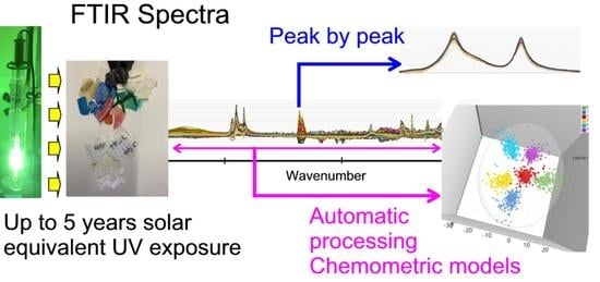
Modelling the Photodegradation of Marine Microplastics by Means of Infrared Spectrometry and Chemometric Techniques

Abstract

This work investigated the structural and chemical changes of plastics undergoing accelerated ageing upon irradiation that simulated the ultraviolet component of solar radiation for a five-year period. The plastics selected were polyethylene (PE) and polypropylene (PP) microplastic debris sampled from a sandy beach as well as pure pellets and fragments of objects made of the same polymers. We recorded Fourier Transform Infrared (FTIR) spectra at prescribed intervals during the irradiation procedure. The spectra were used to study the evolution of the absorption peaks usually associated with the environmental ageing of polyolefins, namely the peaks of hydroxyl and carbonyl stretching, the peaks relating to the presence of double bonds, and those associated with the crystallinity of PE and the tacticity of PP. The results showed that none of the usual degradation indexes followed a clear trend with increasing exposure and that the evolution of absorption peaks was not consistent among different fragments. We used the Orthogonal Partial Least Squares Discriminant Analysis (OPLS-DA) method to process the whole information contained in the FTIR spectra in response to the chemical changes occurring during photochemical ageing. The results showed that the FTIR spectra contained sufficient information to cluster samples according to the irradiation received. Variable Importance of the Projection (VIP) analyses showed that the information for discriminating among different exposures was mainly contained in the absorption peaks corresponding to the hydroxyl and carbonyl stretching absorptions. The chemometric models had large determination coefficients, despite the large number of variables involved and could be applied to assess the environmental fate of plastics under environmental stressors.

1. Introduction

The worldwide production of the different types of plastic has been steadily increasing since the onset of their industrial manufacture to reach a maximum of 368 million tonnes in 2019. In 2020, the production slightly dropped to 367 million tonnes, only one million tonnes less, but this was the first decrease recorded in the history of the plastics industry [1]. In spite of the efforts made to close the plastic cycle, the annual rate of plastic entering the environment is still estimated at about 40 million tonnes from which 11 million tonnes correspond to the macro- and microplastic (MP) waste that reaches the ocean [2]. Another calculation estimated that two-thirds of the plastic ever produced has already been released to the environment. The same study highlighted the unnecessary abuse of plastic by the fact that about 40% of the global plastic production is meant for packaging, mostly for immediate or near immediate disposal [3]. Some sources of plastic pollution are more difficult to avoid, such as the spreading of plastic fragments and synthetic fibres due to the wearing of goods during use [4]. The presence of intentionally added MPs in certain products is another source of pollution, but the accumulation of plastic in environmental compartments is by far a problem of inadequate waste management rather than a limitation associated with plastic itself [5]. In fact, synthetic polymers are extremely useful materials, with unique properties and relatively low energy content making the environmental cost of replacing them with alternatives such as glass, paper or natural substances prohibitive [6].

Plastic disseminated into the environment accumulates due to its chemical persistence, but eventually undergoes degradation and fragmentation processes under environmental stressors. Previous studies have shown that the MPs floating on the sea surface were brittle, which was attributed to the leaching of plasticizers [7]. It has been generally established that photoinitiated oxidative degradation is the main mechanism by which plastics suffer environmental ageing [8]. Photochemical degradation combined with different hydrolysis and oxidation reactions results in the formation of oxygenated moieties such as carboxylic end groups in the fragments resulting from the breaking of polymer backbones [9]. Another problem is that the loss of stabilizer additives affects degradation rate in a different way depending on the exact composition of each plastic item, making it difficult to predict the degradation rates of fragments with different chemical history [8].

Vibrational spectroscopy, in this case infrared (IR), is an ideal tool extensively used for the elucidation of chemical and physical properties of polymers, the qualitative and quantitative analysis of polymer blends, and the tracking of their degradation processes [10]. Bond indexes calculated from FTIR spectra have been used to assess the changes suffered by plastics during weathering. However, their usefulness is limited because of the large variability observed for different plastics and ageing conditions [11]. Our hypothesis is that the information contained in the spectra of aged plastics can be revealed using chemometric modelling. In this work, we used MPs from marine origin and exposed them to accelerated ageing, simulating up to five years of additional UV solar exposure. The MPs consisted of polyethylene (PE) and polypropylene (PP), sampled from a sandy beach as well as pure pellets and fragments of PE and PP obtained from plastic goods. The purpose of this study was to assess the possibility of obtaining information about the environmental history of polyolefin MPs using mid-IR spectroscopy and chemometric techniques.

2. Materials and Methods

2.1. Materials and Experimental Procedure

The environmental plastic fragments used were MPs collected from the sandy beach Ámbar, located in the North coast of La Graciosa, a small island belonging to the Chinijo Archipelago, Canary Islands, Spain. La Graciosa Island is a specially protected area, declared Biosphere Reserve by UNESCO. Accordingly, the beach has very limited human pressure, but it suffers from severe plastic pollution driven with the Canary Current from the North Atlantic Gyre. The MPs sampled from Ámbar beach were mostly PE and PP, which represented 84% and 11% of all plastic particles identified, as shown elsewhere [12]. A total number of 30 marine MP samples (23 PE and 7 PP) were selected with different shapes and colours from the Ámbar beach. Two pure Goodfellow commercial pellets (one low-density polyethylene, LDPE, and one PP) free of additives or charges, in their natural colour, 2–3 mm in size, were also studied. In addition, 4 fragments of PE (LDPE and high-density polyethylene, HDPE) and PP obtained from commercial goods were also used for simulated ageing experiments. The samples were carefully washed with HPLC-grade methanol (CAS 67-56-1, Merck KGaA, Darmstadt, Germany) and ultrapure water (Milli-Q Q-POD Ultrapure Water System) and distributed in four 90 mm diameter glass containers filled with 250 mL simulated seawater, which was prepared according to ASTM D1141-98 using pure chemicals from Merck and Fisher Scientific (Hampton, NH, USA) to reach a final density of 1.025 g/mL measured at 15 °C [13]. The containers were placed on a gyratory shaker operating at 30 rpm for uniform exposure.

Accelerated ageing was simulated using a 150 W medium-pressure mercury lamp (NovaLight TQ150, Peschl Ultraviolet, Mainz, Germany) emitting in the 297–579 nm range. The exposure time was calculated from NASA’s EarthData readings for the Canary Islands (https://power.larc.nasa.gov/data-access-viewer/, accessed 10 November 2021), namely 5.62 kWh m⁻² day⁻¹ (234 W m⁻²), 5% of which corresponds to UVA+UVB (or 280–400 nm). Lamp irradiance was 1350 W m⁻² (UVA+UVB or 280–400 nm) measured using a StellarNet Modular Spectrometer equipped with SpectraWiz OS v5.33 software (StellarNet Inc., Tampa, FL, USA). Therefore, the system needed 74 h of exposure to simulate one year of solar UV irradiation, which were approximated by 3 days of continuous irradiation. The near-UV light quanta (400–290 nm) have energies from 3.1 to 4.3 eV, which correspond to 72–97 kcal/mol, which was sufficient for breaking most of the chemical bonds in the polymer samples [14]. The study was carried out over a total irradiation time of 360 h, simulating five years of solar UVA+UVB exposure.

2.2. Analyses

Measurements were taken from each specimen every 72 h. Samples are denoted in what follows as zero (Y0, initial), and Y1 (72 h) to Y5 (360 h). After every 72 h period, the samples were washed with ultrapure water, dried at 50 °C for 12 h, and stabilized at room temperature for another 12 h before recording FTIR spectra. The spectra were obtained in a Nicolet iS10 Attenuated Total Reflectance Fourier Transform Infrared (ATR-FTIR) apparatus with a Smart iTR-Diamond module and OMNIC software (ThermoFisher Scientific, Waltham, MA USA). The operating parameters were: 4000–650 cm⁻¹ range; 4 cm⁻¹ resolution; and 16 acquisitions (co-added scans). Seven spectra were taken for each sample; hence, 252 spectra were generated for every irradiation time, which resulted in 1512 spectra/sample. This created a matrix of 1512 rows (number of observations/items/objects) and 6950 columns (number of variables/wavelengths) that were analysed using chemometrics tools. The spectra corresponding to Y0 (or initial) were recorded from specimens directly taken from the beach, after cleaning and drying. All changes due to simulated ageing were recorded on that basis and for every individual fragment.

The photodegradation of polyolefins has been shown to start by the photolytic cleavage of chemical bonds in the polymer backbone to form radical pairs (Norrish Type I reaction) or pairs of saturated and unsaturated chain ends (Norrish Type II reaction) [15,16]. The process is followed by the reaction with molecular oxygen to produce peroxy radicals, which abstract hydrogen atoms to form hydroperoxide groups. Hydroperoxides break forming pairs of alkoxy and hydroxyl radicals, which proceed via radical chain mechanisms in a complex series of initiation, propagation, chain branching, and termination reactions [17]. The degradation produces a large variety of oxygenated moieties. Specifically concerning PE, the relevant absorbance peaks in the mid-IR correspond to the ester carbonyl bond at 1740 cm⁻¹, the keto-carbonyl bond at 1715 cm⁻¹, and the terminal and internal double bonds at 1650 cm⁻¹ and 908 cm⁻¹, respectively. The absorbance intensities (I) were computed relative to the methylene bond peak (in plane CH₂ deformation) at 1465 cm⁻¹ using the following expressions [18]:

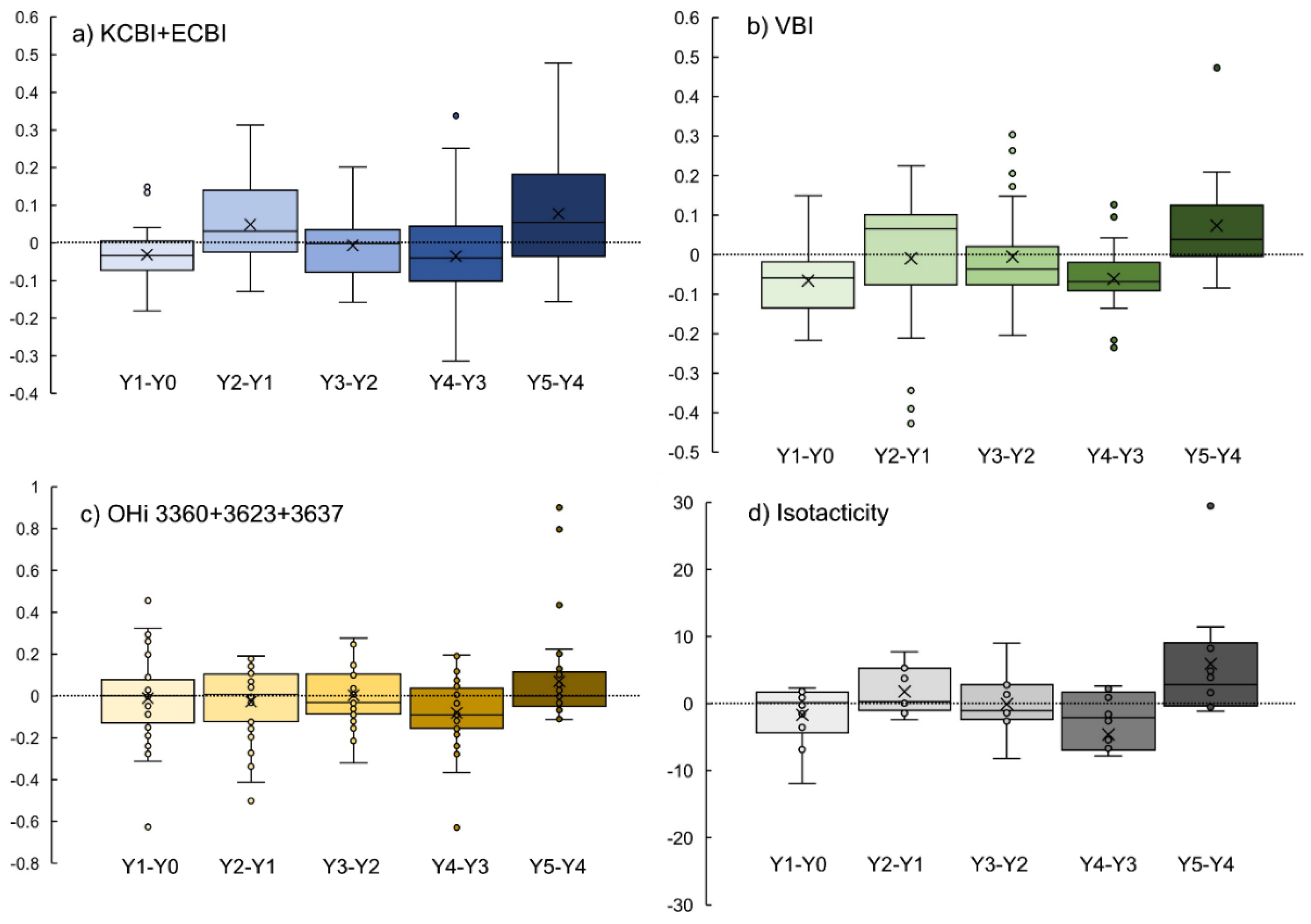
• Keto-Carbonyl Bond Index (KCBI) = I₁₇₁₅/I₁₄₆₅
• Ester-Carbonyl Bond Index (ECBI) = I₁₇₄₀/I₁₄₆₅
• Vinyl Bond Index (VBI) = I₁₆₅₀/I₁₄₆₅
• Internal Double Bond Index (IDBI) = I₉₀₈/I₁₄₆₅

Crystallinity, X_c(%), was measured for PE using the following expression in which I_a and I_b are the absorbance for the bands at 1474 cm⁻¹ and 1464 cm⁻¹, respectively [19]:

$${\mathrm{X}}_{\mathrm{c}}(\%)=100\left[1-\left(\frac{{\mathrm{I}}_{\mathrm{b}}-\frac{{\mathrm{I}}_{\mathrm{a}}}{1.233}}{{\mathrm{I}}_{\mathrm{a}}+{\mathrm{I}}_{\mathrm{b}}}\right)\right]$$

(1)

Concerning PP, the photodegradation process was tracked using the absorbance intensities of ester (1748 cm⁻¹) and methyl (1377 cm⁻¹) groups. The absorbance intensity corresponding to the bending of methylene group at 1456 cm⁻¹ was used as a reference because, as in the case of the 1465 cm⁻¹ peak for PE, the absorbance recorded for the same fragments did not show significant differences (p-value < 0.05). Moreover, the isotacticity index of PP was computed using the bands as 997 cm⁻¹ and 973 cm⁻¹ [20]. Accordingly, the following parameters were calculated:

• Ester-Carbonyl Bond Index (ECBI): I₁₇₄₈/I₁₄₅₆
• Methyl Group Index (MGI): I₁₃₇₇/I₁₄₅₆
• Isotacticity, I(%) computed as (I₉₉₇/I₉₇₃) × 100

The generation of hydroxyl groups during the photodegradation process was assessed by monitoring the evolution of the hydroxyl group band from 3100 cm⁻¹ to 3800 cm⁻¹ [21]. Specifically, we defined three hydroxyl indexes (OHi) computed using the same absorption peak as reference, which was taken at 1465 cm⁻¹ for PE and 1456 cm⁻¹ for PP. The selected wavenumber ranges were: 3360 cm⁻¹ for OH stretching in the case of intramolecular hydrogen bonding, and 3637 cm⁻¹ and 3623 cm⁻¹ for primary and non-primary OH groups.

Before data analysis, all the spectra received a pre-processing transformation using the following sequence: baseline and offset correction, standard normal variate (SNV) normalization, and Savitzky-Golay smoothing (2nd order polynomial and 7 points with symmetric Kernel), using The Unscrambler v10.4 software (AspenTech, Bedford, MA, USA).

2.3. Statistics

The spectral data were analysed using orthogonal partial least squares discriminant analysis (OPLS-DA). OPLS-DA is a statistical modelling tool that provides insights into the separations among experimental groups, in this case, based on data containing high-dimensional spectral measurements with multicollinear and noisy variables [22,23]. This method combines orthogonal signal correction (OSC) and partial least squares discriminant analysis. The goodness of fitting is assessed by means of the cross-validation parameters, R²X, R²Y and Q², representing the explained variance and the predictive capability of the model. R²X and R²Y indicate the fraction of variance of the X and Y matrices, and Q² gives the predictive power of the model. The confidence level of the parameters was set to 95%, and the significance level for the Hotelling’s T² was set to 0.05 [24]. The software also returns the analysis of Variable Importance of the Projection (VIP). These plots summarize the importance of the variables to explain X and correlate Y, the part of X related to Y, and the part of X orthogonal to Y.

3. Results and Discussion

3.1. Photodegradation Indexes

The evolution of degradation indexes, crystallinity, and isotacticity was tracked using seven FTIR spectra per sample and per irradiation time as indicated in the preceding section. The results are shown in Figure S1, and in Tables S1 and S2 (Supplementary Materials, SM) for PE and PP, respectively. Samples before treatment are represented as Y0, while YN stands for samples after irradiation equivalent to N (1 to 5) years of solar UV exposure. The values for the outliers were identified and shown in Table S3 (SM). (Representative spectra before and after irradiation are shown in Figure S2, SM) High values of KCBI and ECBI are observed, for example, for sample PE-Mar-22, for which the intensity was high throughout all the irradiation time. However, most MP fragments did not follow a clear trend, although a maximum in KCBI and ECBI was usually observed after the first 72 h of irradiation, equivalent to one year of solar exposure. The results also showed a slight tendency of PE crystallinity to decrease (Figure S1e). Generally, the crystalline content is expected to increase as a consequence of the higher susceptibility of the amorphous fraction to the photooxidation [25]. However, the results available in the literature do not always show a crystallinity increase with ageing, and in some cases the opposite behaviour has been observed, which could be due to the formation of bulky groups that decrease polymer packing [26]. Concerning PP isotacticity (Figure S1h) the results showed a decrease with irradiation time. This result can be interpreted as the consequence of the formation under oxidation conditions of tertiary radicals in carbon atoms, which temporarily lose their sp³ configurations and, therefore, their stereospecificity [27].

The effect of photochemical ageing on degradation indexes was clearer when depicting changes in indexes, rather than absolute values. Figure 1a,b show Δ(KCBI+ECBI) and Δ(VBI) between two consecutive measurements. A complex pattern could be observed in which carbonyl indexes increased at the beginning and the end of irradiation with a decrease for intermediate exposures. The evolution of OH indexes displayed a slightly downward trend, difficult to appreciate in Figure S1, but depicted clearer in the incremental form of Figure 1c that shows the differences in OHi-3360+3623+3637 between two consecutive one-year irradiation periods. Most of the variability was due to OHi-3360 associated with intramolecular hydrogen bonding, while OH stretching from primary and non-primary alcohols remained with little changes. A similar absence of obvious pattern was observed for PP isotacticity (Figure 1d).

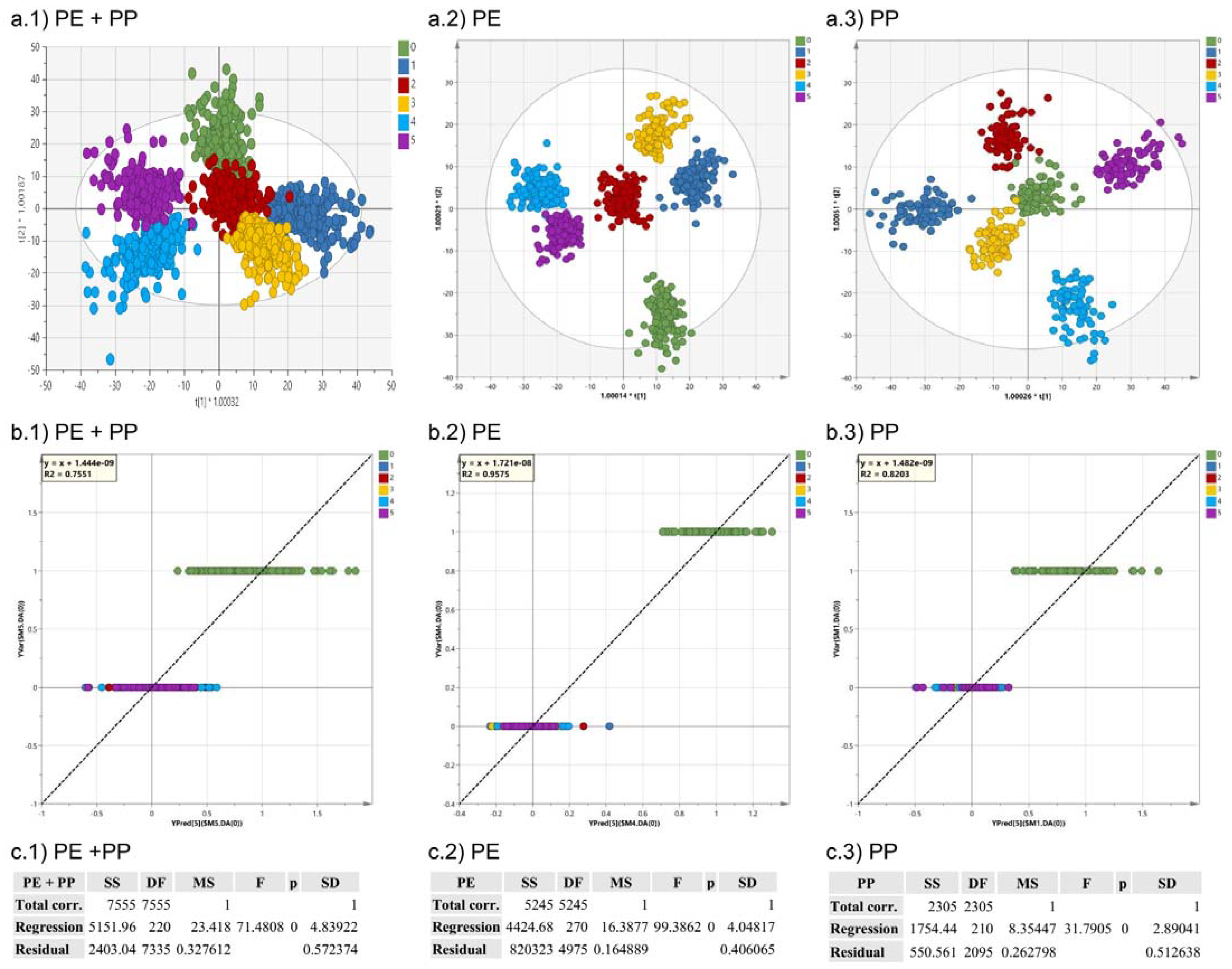
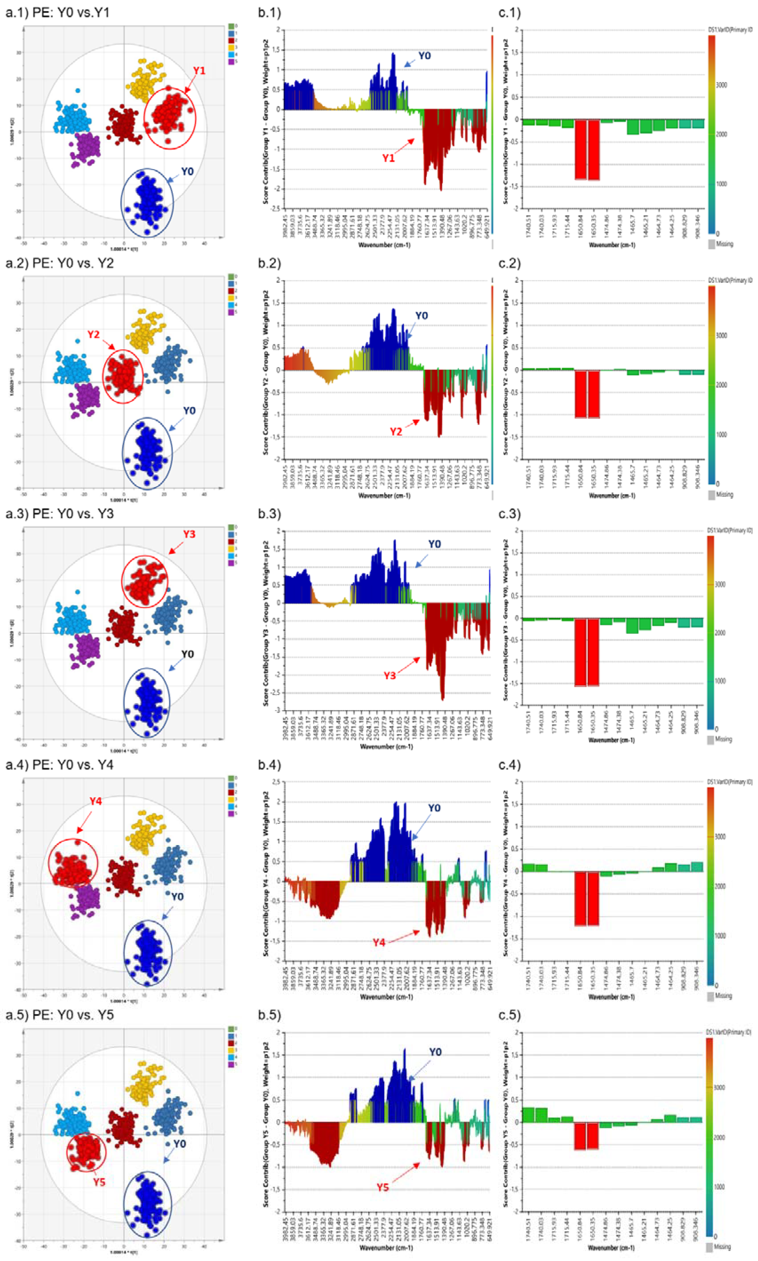
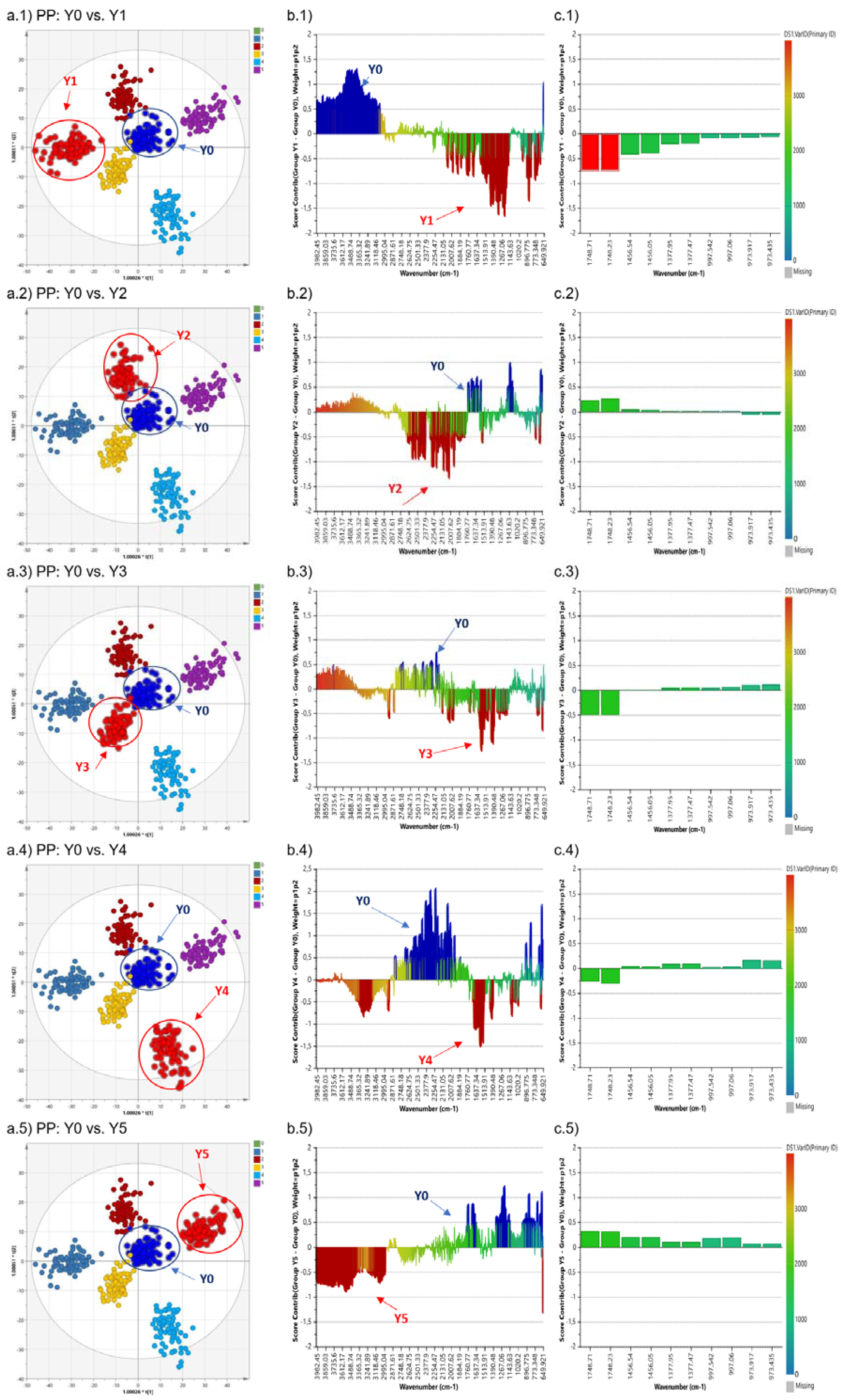
3.2. Orthogonal Partial Least Square-Discriminant Analysis (OPLS-DA)

This study used OPLS-DA with unit variance autoscaling, cross-validation, and autofit modes in the search for the maximum number of valid predictive and orthogonal components. Several models were created using the following classes: Polymer (PE and PP), Origin (new pellets, fragments of objects, and marine debris), Colour (red, green, blue, black, white, and translucent), Irradiation Time (Y0 and YN), and Shape (Fragment [3D], plate [2D], and rod [1D]) [28]. The models calculated for all samples had a root mean square error of estimation (RMSEE) in the 0.033–0.250 range, and a root mean square error of cross validation (RMSECV) in the 0.039–0.367 range. Additional models were calculated for the classes Origin (commercial pellets, fragments of objects, and marine debris) and Polymer (PE and PP). The results are shown in

Table 1. Orthogonal partial least squares discriminant analysis (OPLS-DA) parameters obtained from the different models for all the samples and their subsets by Origin (commercial pellets, fragments of objects, and marine debris) and Polymer (PE and PP).

Id.	Group Class	Spectra	Descriptive Components	Orthogonal Components	R2 X(cum)	R2 Y(cum)	Q2 (cum)	RMSEE	RMSECV
1	All Samples
	Polymer	1512	6	16	0.931	0.749	0.710	0.094	0.102
	Origin	1512	2	13	0.912	0.946	0.938	0.051	0.051
	Colour	1512	5	14	0.926	0.576	0.534	0.250	0.259
	Irradiation Time	1512	5	17	0.932	0.714	0.679	0.186	0.201
	Shape	1512	2	14	0.915	0.967	0.962	0.033	0.367
2	Commercial pellets
	Polymer	84	1	3	0.793	0.977	0.970	0.079	0.087
	Irradiation Time	84	5	5	0.925	0.714	0.602	0.246	0.264
3	Fragments of objects
	Polymer	168	2	6	0.950	0.943	0.912	0.130	0.157
	Colour	168	1	3	0.882	0.970	0.958	0.088	0.103
	Irradiation Time	168	5	3	0.943	0.568	0.497	0.271	0.275
4	Marine debris
	Polymer	1260	1	5	0.832	0.836	0.819	0.178	0.187
	Colour	1260	5	14	0.933	0.565	0.519	0.161	0.185
	Irradiation time	1260	5	17	0.939	0.752	0.710	0.161	0.180
5	PE
	Polymer	1050	3	15	0.921	0.948	0.935	0.044	0.046
	Origin	1050	2	13	0.907	0.962	0.954	0.048	0.049
	Irradiation Time	1050	5	22	0.942	0.888	0.848	0.078	0.110
	Colour	1050	5	13	0.924	0.611	0.556	0.228	0.024
	Shape	1050	2	13	0.906	0.964	0.957	0.046	0.048
6	PP
	Polymer	462	2	11	0.907	0.947	0.916	0.050	0.067
	Origin	462	2	11	0.907	0.947	0.916	0.050	0.067
	Irradiation Time	462	5	16	0.930	0.849	0.774	0.162	0.184
	Colour	462	3	9	0.902	0.755	0.693	0.185	0.210
	Shape	462	1	10	0.896	0.979	0.957	0.042	0.060

.

The effect of photo-oxidative degradation was apparent in the models with the group class Irradiation Time. Figure 2(a.1–a.3) shows the OPLS-DA score scatter plots for PE+PP, PE, and PP at different irradiation times. The plots indicate that the information contained in the FTIR spectra allowed grouping the specimens as a function of UV exposure or irradiation time. This result was evidenced by a relationship between polymer type (projected X dataset) and exposure (Y, categorical variable).

Figure 2(b.1–b.3) show the OPLS-DA predicted vs. observed regression plots for the models. For the PE+PP model, the determination coefficient (R²) was 0.7551, RMSEE was 0.1859, and RMSECV was 0.2010. The fitting parameters improved for PE (R² = 0.9575, RMSEE = 0.0779, and RMSECV = 0.1099) and PP (R² = 0.8203, RMSEE = 0.1614, and RMSECV = 0.1841). These results indicated that the OPLS-DA models were rather robust, with good data fitting. Figure 2(c.1–c.3) display the results for CV-ANOVA analyses based on the cross-validation process for the estimation of independent predictors and predictive residuals. The three models showed a CV-ANOVA p-value < 0.05 confirming the existence of significant differences and supporting the validity and robustness of the three models. Next, the data representing different extent of the photo-oxidation process were selected one by one (Y1, Y2, Y3, Y4, and Y5) and a comparative analysis was performed group by group, against the data before irradiation (Y0). This comparison procedure is summarised in Figure 3(b.1–b.5) for PE, and Figure 4(b.1–b.5) for PP, respectively. These difference plots indicate how much every band (in the respective group) contributed to the model; the larger the band’s bar, the larger its contribution to the model. The contribution threshold was set to 0.5 as default; hence, contribution values > 0.5 are marked in blue for Y0, red for Y1 to Y5, and orange if the bars’ contribution values are larger than 3StdDev (three times the overall standard deviation).

The developed models shed light on the information contained in the absorbance peaks used for the calculation of the degradation indexes. Figure 3 (for PE) and Figure 4 (for PP) show the main changes in the spectra explaining the observed variability. For PE, the differences regarding the bands at 3623 cm⁻¹ and 3637 cm⁻¹ (OH stretching) were significant (score contribution > 0.5) for Y1 and reached the maximum for Y3 (score contribution > 0.75). The opposite correlation was observed for the absorption at 1650 cm⁻¹ attributed to the terminal double bonds. In the case of PP, the absorption corresponding to the OH stretching was very significant after Y1 (score contribution > 0.75) and decreased thereafter until a negative correlation at Y5. In addition, the carbonyl stretching absorption at 1748 cm⁻¹ reached scores > 0.75 for PP after the first year of equivalent exposure (Y1) to follow a complex pattern thereafter.

An additional insight into the drivers of the variance was provided by VIP plots. Figure 5(a.1,b.1,c.1) represent the VIP total plot for the Polymer and Irradiation Time classes in the case of PE+PP, PE, and PP, respectively. Figure 5(a.2,b.2,c.2) represent the VIP predictive plots for the same models. Figure 5(a.3,b.3,c.3) represent VIP orthogonal plots.

The next step was to quantitatively determine the discriminating power of wavenumber in the classification process. VIP plots required selecting the peaks used for index’s calculation in their respective models (PE+PP, PE, and PP). Peaks with VIP > 1 were considered explanatory for the model. VIP total plot showed that the explanatory peaks were those at 1650 cm^–1, 1715 cm^–1, and 1740 cm⁻¹ for PE, and 1748 cm⁻¹ for PP. However, other peaks, with VIP in the 0.5–1 range could be considered moderately significant. This was the case for 1377 cm⁻¹ for PE+PP and 973 cm⁻¹ for PP, both used in the PP indexes’ calculation (MGI and Isotacticity). None of the reference peaks (1465 cm⁻¹, 1456 cm⁻¹, and 973 cm⁻¹) conveyed degradation information, which confirmed that their selection was correct.

Our results showed that the information provided by the degradation indexes based on certain peaks of the FTIR spectra cannot be directly correlated with the environmental photodegradation history, at least for different plastic particles. A maximum in the degradation indexes associated with the carbonyl bond stretching was produced as an intermediate degradation step, but further irradiation led to a non-uniform evolution of indexes based on that absorption band. Likewise, the hydroxyl bond-related indexes did not follow a clear pattern except when tracking the evolution of individual particles. Accordingly, our results showed that simple degradation indexes, although extensively used in the past to assess the extent of plastic photodegradation, cannot be generally accepted as an indication of the accumulated exposure of plastic debris to photochemical ageing. The use of specific IR bands to quantitatively assess the oxidation extent of polyolefins has already been criticized because the evolution of chemical bonds upon weathering do not change linearly with time [11]. The mere evolution of certain peaks cannot be related in a simple way with the environmental stress suffered by the plastic except when analysing the same fragment due to the huge variability observed for different plastics (even with the same polymer), weathering conditions, and bond type determined. However, the information about plastic ageing is still contained in the mid-infrared spectra and can be revealed using OPLS-DA models, which allowed discriminating among samples depending on the irradiation received in accelerated ageing experiments. The relationship between photochemical ageing and individual FTIR bands was not simple, and several peaks were involved. Nevertheless, the samples with different exposure times were clearly discriminated from each other. The information for the discrimination was contained mostly in the absorption bands mainly corresponding to the hydroxyl and carbonyl bond stretching. The use of full spectral information combination offers the possibility of sorting plastic debris as a function of their irradiation history.

4. Conclusions

Infrared Spectrometry and Chemometric techniques were used to model the photodegradation of marine litter polymers. The selected materials were PE and PP microplastics recovered from a sandy beach as well as pure pellets and fragments of objects made of the same polymers, which were subject to accelerated ageing that delivered UV irradiation equivalent to up to five years or solar exposure.

Degradation indexes were calculated by tracking the absorbance peaks from carbonyl, hydroxyl, and double bonds, as well as peak ratios measuring crystallinity (PE) and tacticity (PP). The results showed that none of the degradation indicators yielded a clear trend as a function of UV exposure. Even without considering outliers, the evolution of IR absorption peaks was different for different specimens and did not follow a simple pattern.

OPLS-DA models were used to process all the information contained in ATR-FTIR spectra. The models allowed clustering both polymers in different classes according to the irradiation received in accelerated ageing experiments. VIP analyses showed that the information for the discrimination was mainly contained in the absorption peaks corresponding to the hydroxyl and carbonyl stretching absorptions, with lower contribution from the peaks associated with vinyl bonds (PE) and tacticity (PP). Although the models were derived from a large set of variables, the chemometric models presented good fitting and can be used for prediction.

References

1. PlasticsEurope. Plastics—The Facts 2021: An Analysis of European Plastics Production, Demand and Waste Data; PlasticsEurope; Association of Plastics Manufacturers: Brussels, Belgium, 2021. [Google Scholar]
2. Lau, W.W.Y.; Shiran, Y.; Bailey, R.M.; Cook, E.; Stuchtey, M.R.; Koskella, J.; Velis, C.A.; Godfrey, L.; Boucher, J.; Murphy, M.B.; et al. Evaluating scenarios toward zero plastic pollution. Science 2020, 369, 1455–1461. [Google Scholar] [CrossRef] [PubMed]
3. Pinto-da-Costa, J.; Rocha-Santos, T.; Duarte, A.C. The Environmental Impacts of Plastics and Micro-Plastics Use, Waste and Pollution: EU and National Measures; European Union; Policy Department for Citizens’ Rights and Constitutional Affairs: Brussels, Belgium, 2020; pp. 1–72. [Google Scholar]
4. Napper, I.E.; Thompson, R.C. Release of synthetic microplastic plastic fibres from domestic washing machines: Effects of fabric type and washing conditions. Mar. Pollut. Bull. 2016, 112, 39–45. [Google Scholar] [CrossRef] [PubMed] [Green Version]
5. OECD. Global Plastics Outlook: Economic Drivers, Environmental Impacts and Policy Options; OECD Publishing: Paris, France, 2022. [Google Scholar] [CrossRef]
6. North, E.J.; Halden, R.U. Plastics and environmental health: The road ahead. Rev. Environ. Health 2013, 28, 1–8. [Google Scholar] [CrossRef] [PubMed]
7. Carpenter, E.J.; Smith, K.L. Plastics on the Sargasso Sea surface. Science 1972, 175, 1240–1241. [Google Scholar] [CrossRef]
8. Chamas, A.; Moon, H.; Zheng, J.; Qiu, Y.; Tabassum, T.; Jang, J.H.; Abu-Omar, M.; Scott, S.L.; Suh, S. Degradation rates of plastics in the environment. ACS Sustain. Chem. Eng. 2020, 8, 3494–3511. [Google Scholar] [CrossRef] [Green Version]
9. Gewert, B.; Plassmann, M.M.; MacLeod, M. Pathways for degradation of plastic polymers floating in the marine environment. Environ. Sci. Processes Impacts 2015, 17, 1513–1521. [Google Scholar] [CrossRef] [Green Version]
10. Gopanna, A.; Mandapati, R.N.; Thomas, S.P.; Rajan, K.; Chavali, M. Fourier transform infrared spectroscopy (FTIR), Raman spectroscopy and wide-angle X-ray scattering (WAXS) of polypropylene (PP)/cyclic olefin copolymer (COC) blends for qualitative and quantitative analysis. Polym. Bull. 2019, 76, 4259–4274. [Google Scholar] [CrossRef]
11. Brandon, J.; Goldstein, M.; Ohman, M.D. Long-term aging and degradation of microplastic particles: Comparing in situ oceanic and experimental weathering patterns. Mar. Pollut. Bull. 2016, 110, 299–308. [Google Scholar] [CrossRef] [Green Version]
12. Edo, C.; Tamayo-Belda, M.; Martínez-Campos, S.; Martín-Betancor, K.; González-Pleiter, M.; Pulido-Reyes, G.; García-Ruiz, C.; Zapata, F.; Leganés, F.; Fernández-Piñas, F.; et al. Occurrence and identification of microplastics along a beach in the Biosphere Reserve of Lanzarote. Mar. Pollut. Bull. 2019, 143, 220–227. [Google Scholar] [CrossRef]
13. ASTM D1141-98(2021); Standard Practice for Preparation of Substitute Ocean Water. ASTM International: West Conshohocken, PA, USA, 2021. [CrossRef]
14. Rånby, B. Photodegradation and photo-oxidation of synthetic polymers. J. Anal. Appl. Pyrolysis 1989, 15, 237–247. [Google Scholar] [CrossRef]
15. Jabarin, S.A.; Lofgren, E.A. Photooxidative effects on properties and structure of high-density polyethylene. J. Appl. Polym. Sci. 1994, 53, 411–423. [Google Scholar] [CrossRef]
16. Singh, B.; Sharma, N. Mechanistic implications of plastic degradation. Polym. Degrad. Stab. 2008, 93, 561–584. [Google Scholar] [CrossRef]
17. Agboola, O.; Sadiku, R.; Mokrani, T.; Amer, I.; Imoru, O. Polyolefins and the environment. In Polyolefin Fibres, 2nd ed.; Ugbolue, S.C.O., Ed.; Woodhead Publishing: Sawston, UK, 2017; pp. 89–133. [Google Scholar]
18. Albertsson, A.-C.; Andersson, S.O.; Karlsson, S. The mechanism of biodegradation of polyethylene. Polym. Degrad. Stab. 1987, 18, 73–87. [Google Scholar] [CrossRef]
19. Zerbi, G.; Gallino, G.; Del Fanti, N.; Baini, L. Structural depth profiling in polyethylene films by multiple internal reflection infra-red spectroscopy. Polymer 1989, 30, 2324–2327. [Google Scholar] [CrossRef]
20. Arkatkar, A.; Arutchelvi, J.; Bhaduri, S.; Uppara, P.V.; Doble, M. Degradation of unpretreated and thermally pretreated polypropylene by soil consortia. Int. Biodeterior. Biodegrad. 2009, 63, 106–111. [Google Scholar] [CrossRef]
21. Adothu, B.; Costa, F.R.; Mallick, S. Damp heat resilient thermoplastic polyolefin encapsulant for photovoltaic module encapsulation. Sol. Energy Mater. 2021, 224, 111024. [Google Scholar] [CrossRef]
22. Chung, I.-M.; Kim, J.-K.; Han, J.-G.; Kong, W.-S.; Kim, S.-Y.; Yang, Y.-J.; An, Y.-J.; Kwon, C.; Chi, H.-Y.; Yhung Jung, M.; et al. Potential geo-discriminative tools to trace the origins of the dried slices of shiitake (Lentinula edodes) using stable isotope ratios and OPLS-DA. Food Chem. 2019, 295, 505–513. [Google Scholar] [CrossRef] [PubMed]
23. Worley, B.; Powers, R. PCA as a practical indicator of OPLS-DA model reliability. Curr. Metab. 2016, 4, 97–103. [Google Scholar] [CrossRef] [Green Version]
24. Bylesjö, M.; Rantalainen, M.; Cloarec, O.; Nicholson, J.K.; Holmes, E.; Trygg, J. OPLS discriminant analysis: Combining the strengths of PLS-DA and SIMCA classification. J. Chemom. 2006, 20, 341–351. [Google Scholar] [CrossRef]
25. Hiejima, Y.; Kida, T.; Takeda, K.; Igarashi, T.; Nitta, K.-h. Microscopic structural changes during photodegradation of low-density polyethylene detected by Raman spectroscopy. Polym. Degrad. Stab. 2018, 150, 67–72. [Google Scholar] [CrossRef]
26. Carrasco, F.; Pagès, P.; Pascual, S.; Colom, X. Artificial aging of high-density polyethylene by ultraviolet irradiation. Eur. Polym. J. 2001, 37, 1457–1464. [Google Scholar] [CrossRef]
27. Iedema, P.D.; Remerie, K.; Seegers, D.; McAuley, K.B. Tacticity changes during controlled degradation of polypropylene. Macromolecules 2021, 54, 8921–8935. [Google Scholar] [CrossRef]
28. Rosal, R. Morphological description of microplastic particles for environmental fate studies. Mar. Pollut. Bull. 2021, 171, 112716. [Google Scholar] [CrossRef] [PubMed]
Figure 1. Variation in degradation indexes every 72 h of irradiation (equivalent to one year of solar exposure) for (a) KCBI-Keto Carbonyl Bond Index + ECBI-Ester Carbonyl Bond Index for PE; and (b) VBI-Vinyl Bond Index for PE; (c) Variation of Hydroxyl Bond Indexes for PE and PP (all specimens); and (d) Changes in PP Isotacticity.
Microplastics 01 00013 g001
Figure 2. OPLS-DA score scatter plots for the models with PE and PP together (a.1), PE (a.2), and PP (a.3); OPLS-DA Predicted vs. Observed plots for the PE+PP (b.1), PE (b.2), and PP (b.3) models; and CV-ANOVA parameters for the models PE+PP (c.1), PE (c.2), and PP (c.3) models.
Microplastics 01 00013 g002
Figure 3. Discrimination sequence for the PE models (rows). OPLS-DA score scatter plots showing the two selected groups being compared (left column); contribution (comparison) plots for the pair of selected groups (centre column), where the most important bands (contribution values > 0.5) are marked in blue for Y0, red for Y1 to Y5, and orange if the bars contribution values are larger than 3StdDev (StdDev = overall standard deviation); and contribution (comparison) plots for the selected variables from every group (right column). According to that sequence, the PE groups were compared as follows (from top of bottom): Y0 vs. Y1 (a.1,b.1,c.1), Y0 vs. Y2 (a.2,b.2,c.2), Y0 vs. Y3 (a.3,b.3,c.3), Y0 vs. Y4 (a.4,b.4,c.4), and Y0 vs. Y5 (a.5,b.5,c.5).
Microplastics 01 00013 g003
Figure 4. Discrimination sequence for the PP models (rows). OPLS-DA score scatter plots showing the two selected groups being compared (left column); contribution (comparison) plots for the pair of selected groups (centre column), where the most important bands (contribution values > 0.5) are marked in blue for Y0, red for Y1 to Y5, and orange if the bars’ contribution values are larger than 3StdDev (StdDev = overall standard deviation); and contribution (comparison) plots for the selected variables from every group (right column). According to that sequence, the PP groups were compared as follows (from top of bottom): Y0 vs. Y1 (a.1,b.1,c.1), Y0 vs. Y2 (a.2,b.2,c.2), Y0 vs. Y3 (a.3,b.3,c.3), Y0 vs. Y4 (a.4,b.4,c.4), and Y0 vs. Y5 (a.5,b.5,c.5).
Microplastics 01 00013 g004
Figure 5. Discrimination sequence for every model (row): VIP total plot (left column), VIP predictive plot (central column), and VIP orthogonal plot (right column). The compared models were (from top to bottom): PE+PP-Irradiation Time (a.1a.3), PE-Irradiation Time (b.1b.3), and PP-Irradiation Time (c.1c.3). The most important bands (contribution values > 0.5) are sorted in descendent order and marked in blue for Y0, red for Y1 to Y5, and orange if the bars contribution values are larger than 3StdDev (StdDev = overall standard deviation).
Microplastics 01 00013 g005