Round-Trip Time Estimation Using Enhanced Regularized Extreme Learning Machine

Abstract

Reliable Internet connectivity is essential for latency-sensitive services such as video conferencing, media streaming, and online gaming. Round-trip time (RTT) is a key indicator of network performance and is central to setting retransmission timeout (RTO); inaccurate RTT estimates may trigger unnecessary retransmissions or slow loss recovery. This paper proposes an Enhanced Regularized Extreme Learning Machine (RELM) for RTT estimation that improves generalization and efficiency by interleaving a bidirectional log-step heuristic to select the regularization constant C. Unlike manual tuning or fixed-range grid search, the proposed heuristic explores C on a logarithmic scale in both directions ($\times 10$ and /10) within a single loop and terminates using a tolerance–patience criterion, reducing redundant evaluations without requiring predefined bounds. A custom RTT dataset is generated using Mininet with a dumbbell topology under controlled delay injections (1–1000 ms), yielding 1000 supervised samples derived from 100,000 raw RTT measurements. Experiments follow a strict train/validation/test split (6:1:3) with training-only standardization/normalization and validation-only hyperparameter selection. On the controlled Mininet dataset, the best configuration (ReLU, 150 hidden neurons, $C={10}^2$) achieves $R^2=0.9999$, $MAPE=0.0018$, $MAE=966.04$, and $RMSE=1589.64$ on the test set, while maintaining millisecond-level runtime. Under the same evaluation pipeline, the proposed method demonstrates competitive performance compared to common regression baselines (SVR, GAM, Decision Tree, KNN, Random Forest, GBDT, and ELM), while maintaining lower computational overhead within the controlled simulation setting. To assess practical robustness, an additional evaluation on a public real-world WiFi RSS–RTT dataset shows near-meter accuracy in LOS and mixed LOS/NLOS scenarios, while performance degrades markedly under dominant NLOS conditions, reflecting physical-channel limitations rather than model instability. These results demonstrate the feasibility of the Enhanced RELM and motivate further validation on operational networks with packet loss, jitter, and path variability.

1. Introduction

A reliable internet connection is essential in the digital era, becoming indispensable for activities such as online shopping, business meetings, and education [1]. Many applications and services, including video conferencing, media streaming, and online gaming, depend heavily on network quality [2,3,4]. One key metric for evaluating network performance is RTT [2,3,5,6]. RTT is the time interval between the sender and receiver, during which packets are sent and acknowledged [4,7], confirming that the data has arrived intact [2,8,9,10]. RTT helps identify network communication delays and is crucial for assessing network performance [1,2,5]. High RTT values indicate suboptimal network performance, inefficient traffic, and delays that negatively affect the user experience [3]. RTT is vital to many reliable transport protocols [8,11], and accurately estimating it is essential for determining the optimal RTO value. RTO defines how long the sender waits before considering a packet lost and retransmitting it. If RTO is too short, unnecessary retransmissions can degrade network performance; if it’s too long, delays in detecting lost packets occur. Without an estimated RTT, network service quality may suffer, performance can decrease, and delays may increase across the network.

Industry data further emphasizes the importance of minimizing RTT. Stadnik et al. [12] mentioned that a 100-ms delay in page load time can reduce conversion rates by 7%, while a two-second delay increases bounce rates by 103%. Additionally, 53% of mobile site visitors abandon pages that take more than three seconds to load. Galetta et al. [13] voiced that a one-second delay in loading can reduce user satisfaction by 16%, affecting trust and retention. These findings highlight that even small increases in latency can significantly impact the digital experience, making RTT not only a network metric but also a key factor in user experience. Liborio et al. [14] said that Cisco’s Annual Internet Report supports this trend, indicating that while global internet speeds are expected to improve to 110.4 Mbps for fixed broadband and 43.9 Mbps for mobile by 2023, latency remains a significant bottleneck. Laniewski et al. [15] reported that median mobile and fixed internet speeds increased by 18.5% and 13.1%, respectively, from 2024 to 2025; however, latency improvements have not kept pace. Furthermore, Kaseng et al. [16] reported that the number of Internet users in Peru increased by 4.3%, from 91 per household to 95. These trends suggest that RTT optimization is no longer a theoretical issue but a growing operational challenge in today’s high-demand network environments.

Given these challenges, many studies have attempted to estimate RTT using various approaches. Chong et al. [17] and Dong et al. [9] applied neural network-based models with promising accuracy; however, both utilized simple peer-to-peer architectures with limited complexity. Jacobsson et al. [8] addressed overfitting using Kalman filters, yet required manual parameter tuning, making their model less suitable for real-time congestion control. These methods demonstrate potential but still face significant limitations in terms of scalability, robustness, and practicality.

Recent advancements in machine learning, notably Extreme Learning Machine (ELM)-based approaches, have shown promise in overcoming the limitations of earlier RTT estimation methods. ELM models are known for their computational efficiency and compact structure, making them ideal for real-time network applications. Liu et al. [18] introduced Functional ELM (FELM), which improved generalization by eliminating the reliance on randomly initialized weights. However, FELM faced scalability challenges when applied to larger datasets and required complex functional formulations. Building on this, Qin Wu et al. [19] introduced L1-ACELM, combining L1-norm regularization with asymmetric C-loss functions to reduce overfitting and improve noise tolerance. Despite its robustness, L1-ACELM’s non-convex optimization process led to iterative training, slowing the typical speed advantages of ELM. Other studies, such as those by Priya et al. [20], Yildirim et al. [21], and Wei et al. [22], proposed enhanced regularization techniques; however, these still required manual parameter tuning and lacked adaptive mechanisms, thereby limiting their real-time applicability. Further advancements, such as RELM and RRELM, have addressed scalability and adaptability issues, thereby improving robustness and noise tolerance, particularly in high-dimensional data, and effectively handling outliers. Online learning approaches, such as IRELM [23], also offer real-time adjustments to evolving network conditions, making them ideal for RTT estimation and network intrusion detection.

Despite significant advancements, current machine learning and statistical methods for RTT estimation still exhibit key limitations, including static architectures, overfitting, and inefficient parameter tuning. These challenges hinder their practical deployment in real-world, dynamic network environments, where models need to be not only accurate but also adaptable, efficient, and scalable.

This research addresses these gaps by proposing an enhanced RELM model with an automated algorithm for selecting the regularization constant. By incorporating a dynamic, adaptive regularization mechanism, the model demonstrates improved stability and reduced sensitivity to parameter tuning under varying simulated delay and traffic conditions. Within this controlled evaluation setting, the approach aims to support latency-sensitive prediction tasks while maintaining computational efficiency and scalability.

• The main contributions are as follows:

• We construct a controlled RTT dataset in Mininet (dumbbell topology) with systematic delay injections (1–1000 ms), producing 1000 supervised samples derived from 100,000 raw RTT measurements.
• We implement an adaptive log-step heuristic (greedy decade search) for selecting the RELM regularization constant C using validation RMSE with a tolerance–patience stopping rule, reducing the number of grid-search evaluations required in practice.
• We benchmark RELM against representative regression baselines using the proposed C-selection heuristic under a leakage-free evaluation pipeline, and we complement the simulation study with an additional evaluation on a public real-world WiFi RTT dataset (LOS/NLOS) to assess behavior under measurement noise and propagation effects.

The remainder of the paper follows this organization: Section 2 discusses state-of-the-art issues related to RTT estimation. In Section 3, we present our workflow and associated theories. Section 4 is where we show the testing results and benchmark them with state-of-the-art research. Lastly, Section 5 finalizes the paper by answering the research aim.

2. Review of Literature and Studies

Numerous studies have been conducted to estimate RTT values in various network environments. These can generally be categorized into four methodological groups: neural network-based approaches, filtering-based methods, hybrid models, and ELM-based techniques. In neural network-based approaches, LSTM and CNN-based models have also been explored. Dasgupta et al. [24] demonstrated that LSTM-CNN networks can significantly reduce retransmissions. However, training such models requires extensive computation up to 100 epochs, exceeding the efficiency of classical estimation algorithms. Hagos et al. [25] further validated LSTM performance across various TCP variants, achieving MAPE values as low as 0.63%, yet their approach depends heavily on TCP timestamps and consistent network conditions.

Nunes et al. [26] proposed a fixed-share expert framework that dynamically assigns weights to multiple predictors. Their method improved accuracy by over 40% compared to standard TCP RTT estimators; however, the underlying learning mechanism still assumes stable trends in prediction error, which limits responsiveness to abrupt RTT shifts.

Filtering-based estimation has received attention for its ability to smooth RTT trends. Guodong et al. [27] applied adaptive filtering and achieved a 93.1% accuracy rate, correctly predicting over 2400 of 2603 samples. However, the algorithm struggled with abrupt RTT spikes because it relied on historical values. Other research introduced a variety of filtering approaches, such as Kalman filtering and adaptive Kalman filtering, that can reduce estimation error.

Expanding into hybrid approaches, Damaševičius et al. [28] integrated ANN with fuzzy logic to create a neuro-fuzzy RTT prediction system. The model achieved an accuracy of 79.36% and supported short-term forecasting for cloud server communications. Mohammed et al. [29] proposed a neural network model for estimating distributed network latency in real-time. Although highly accurate (96.1%, RMSE = 0.053), its performance depends heavily on high-quality input data and is inconsistent under volatile network conditions.

ELM methods have gained popularity due to their fast computation and compact structure. Liu et al. [18] introduced FELM, which eliminates the dependence on randomly initialized weights and improves generalization. However, it lacked scalability testing on large datasets and required complex functional formulations.

Qin Wu et al. [19] developed L1-ACELM, which combines L1-norm robustness with asymmetric C-loss functions to address overfitting and noise. Although robust, its non-convex optimization required iterative training, which undermined the original ELM’s speed advantage. Other efforts, such as those by Priya et al. [20], Yildirim et al. [21], and Wei et al. [22], proposed improved regularization methods (e.g., L1/2 smoothing) but continued to rely on manual parameter tuning and lacked adaptive mechanisms under varying network dynamics.

3. Research Methodology

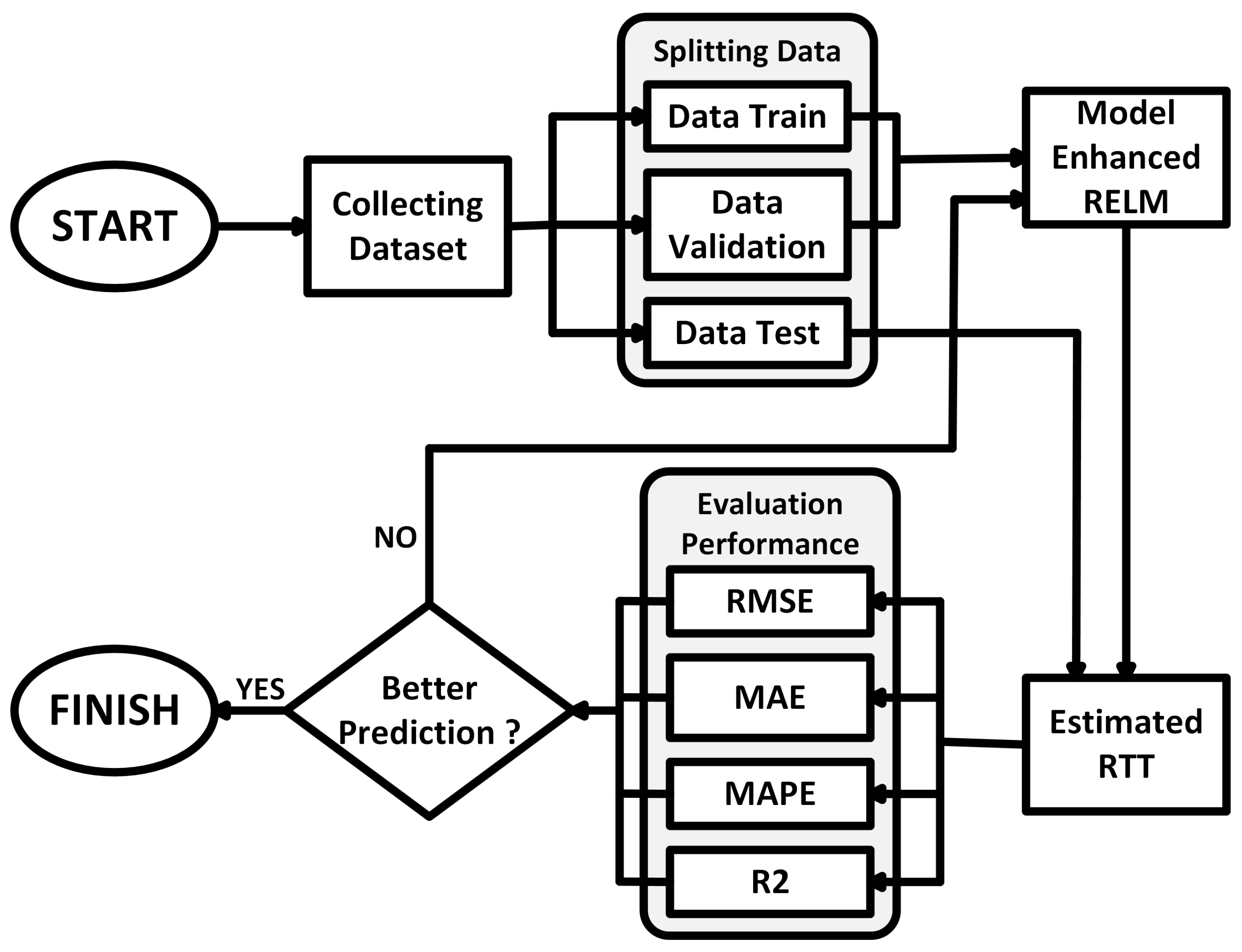
The flowchart in Figure 1 explains the research methodology. This section presents the architecture of the proposed solution, including input selection, data preprocessing, the RELM model design, and evaluation metrics. The emphasis is on addressing the research gap by enabling the model to estimate RTT values efficiently while adapting to diverse conditions.

3.1. Data Collection and Dataset Splitting

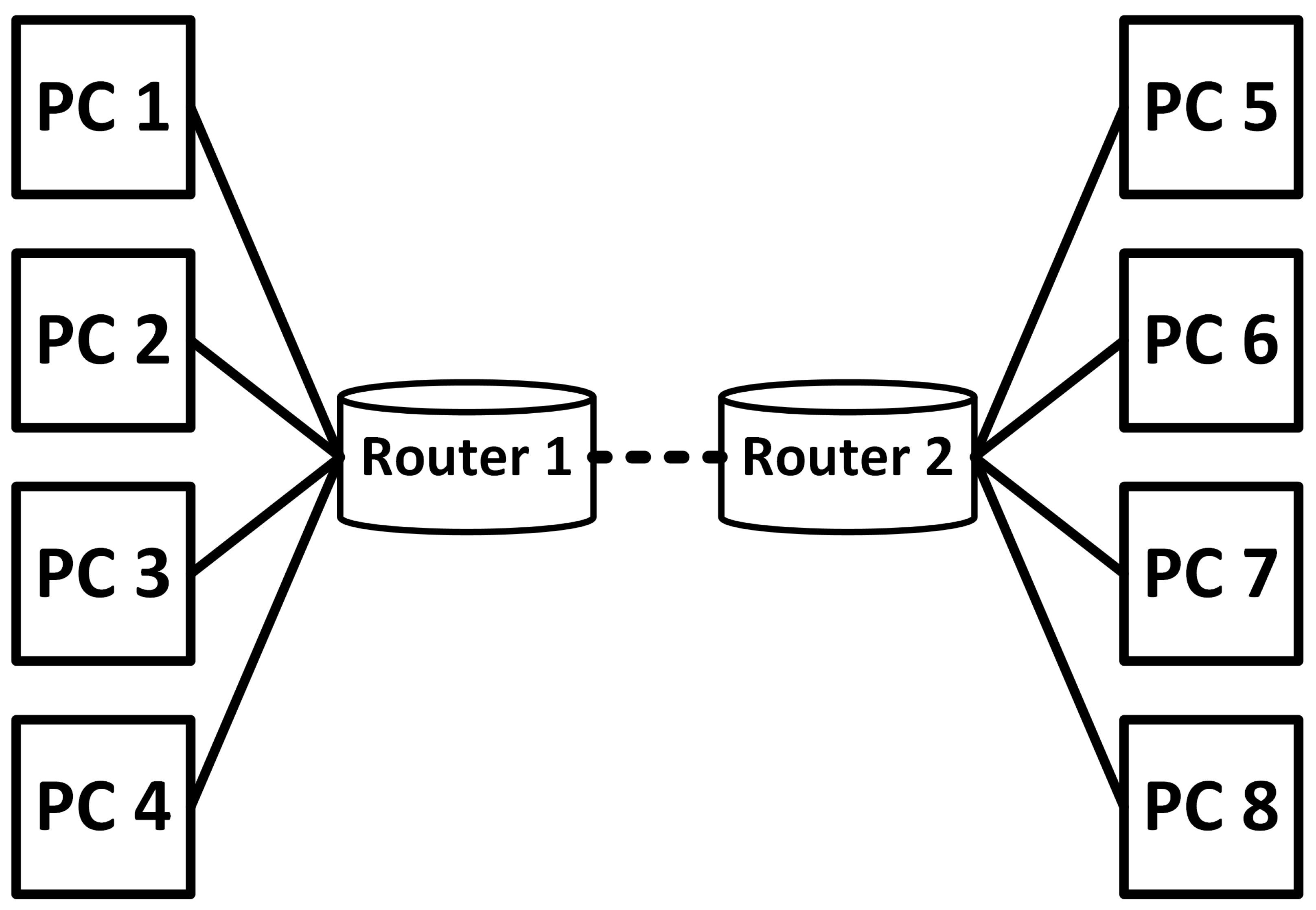
The first step is to create the dataset. A virtual topology was developed using Mininet on Ubuntu within the VirtualBox environment [30,31]. The topology consisted of four hosts and two main routers, connected by a single backbone line, forming a dumbbell topology, commonly used in congestion control experiments [32,33]. Messages were sent between hosts with varying delays, and the RTT, including the time taken, source and destination addresses, next_seq, unacknowledged, congestion window, source window, and receive window, was recorded [34]. The program was run 1000 times with injected delays ranging from 1 ms to 1000 ms. For each run, we recorded 100 RTT measurements (raw records), resulting in 100,000 RTT records in total. For the supervised regression experiments, we then constructed 1000 samples by aggregating the 100 RTT measurements per run (e.g., mean RTT) and pairing them with the corresponding TCP-state features (next_seq, unacknowledged, congestion window, source window, and receive window). Thus, the learning pipeline uses 1000 samples, while 100,000 refers to the number of raw RTT records collected.

The architecture of dumbbell topology in Figure 2 is widely used in modern network architectures for various domains such as home networks, transportation systems, and medical systems [35,36]. It is also used in TCP traffic flow analysis to evaluate congestion control algorithms that affect traffic reliability and performance degradation caused by packet loss [37]. The flexibility and applicability of the dumbbell topology make it ideal for congestion control analysis and throughput fairness evaluation, rendering it a fundamental structure for network simulation, particularly in evaluating TCP traffic flow and congestion management algorithms [38].

The data was split into training, validation, and test sets to train the model, assess its performance during training, and evaluate the final model’s effectiveness. The dataset consisted of 1000 samples, with 600 used for training, 100 for validation, and 300 for testing. Thus, the data distribution ratio was 6:1:3 for training, validation, and test data, respectively. To prevent data leakage, each sample index belongs to exactly one split (train/validation/test) with no overlap. All hyperparameters are selected based solely on the training/validation data. The test set is held out and used only once for final reporting.

RTT represents the time interval between the sender and the receiver during which packets are sent and an acknowledgment is returned, confirming the integrity of the received data. RTT is a crucial metric for measuring network performance, as it helps identify delays in data packet transmission. High RTT values indicate suboptimal network performance and inefficiency in traffic flow, resulting in delays that negatively impact the user experience. Therefore, accurately estimating RTT is essential for optimizing network architecture and improving communication protocols.

Experimental Setup and Runtime Measurement

All experiments were executed on a laptop workstation running Windows 11 Home Single Language 64-bit (Build 26200), equipped with an AMD Ryzen 5 8645HS CPU and 16 GB RAM, using MATLAB R2025b. Runtime is reported in seconds as wall-clock time measured by tic/toc.

To avoid ambiguity, we report three timing components consistently throughout the paper: (i) Train/Tune time: model fitting on the training set, including the C-selection heuristic when applicable (validation-only selection); (ii) Validation time: forward evaluation on the validation set used for model selection (no refitting on validation); (iii) Testing time: forward evaluation on the held-out test set used only once for final reporting. Unless stated otherwise, Testing time refers to processing the full test split (300 samples) and computing metrics after de-normalization.

3.2. The Proposed Enhanced RELM

The fundamental concept of ELM is the random assignment of input weights and hidden-layer biases, followed by a least-squares solution that depends on the target output, the hidden-layer activations, and the activation function [39,40]. The following equation defines the mathematical model:

$$\sum _{i=1}^L{\beta }_i{g}_i\left(x_i\right)=\sum _{i=1}^L{\beta }_i{g}_i(w_i\times x_i+b_i)=y_i$$

(1)

where $w_i={[w_{i1},w_{i2},\dots ,w_{im}]}^T$ is a randomly initialized weight between the input node and the hidden layer, $x_i={[x_{i1},x_{i2},\dots ,x_{im}]}^T\in {\mathbb{R}}^m$ is input in the form of RTT values that have been generated previously, $y_i={[y_{i1},y_{i2},\dots ,y_{im}]}^T\in {\mathbb{R}}^m$ is the result of the RTT value prediction [41,42]. L is the size of the hidden layer, $g\left(x\right)$ is the activation function, and ${\beta }_i={[{\beta }_{i1},{\beta }_{i2},\dots ,{\beta }_{im}]}^T$ is the output weight between the hidden layer and the output node [43].

Furthermore, we can write the above equation compactly as follows:

$$H\beta =y$$

(2)

where

$$\begin{array}{cc}\hfill & H(w_1,\dots ,w_n;b_1,\dots ,b_n;x_1,\dots ,x_n)=\hfill \\ \hfill & \left[\begin{array}{ccc}g(w_{11}·x_{11}+b_1)& \dots & g(w_{1n}·x_{1n}+b_n)\\ g(w_{21}·x_{21}+b_1)& \dots & g(w_{2n}·x_{2n}+b_n)\\ ⋮& ⋮& ⋮\\ g(w_{m1}·x_{m1}+b_1)& \dots & g(w_{mn}·x_{mn}+b_n)\end{array}\right]\hfill \end{array}$$

(3)

$$\beta =\left[\begin{array}{c}{\beta }_1^T\\ ⋮\\ {\beta }_N^T\end{array}\right],\beta \in {\mathbb{R}}^{\overline{N}\times m}$$

(4)

$$T=\left[\begin{array}{c}{T}_1^T\\ ⋮\\ T_N^T\end{array}\right],T\in {\mathbb{R}}^{\overline{N}\times m}$$

(5)

By solving analytically, we can figure out the output weights ($\beta$) with a least squares solution that is:

$$\beta =H^{†}y$$

(6)

where $H^{†}$ denotes the turned Penrose pseudoinverse of H, and H is the hidden-layer output matrix.

In this study, we employed the RELM method as the estimation approach. RELM is an extension of ELM that uses a regularization constant on the output weights to prevent overfitting by limiting the model’s complexity and tailoring it to the training data, thereby enhancing its ability to generalize to new data. This regularization technique treats all features as essential and preserves all information without overfitting.

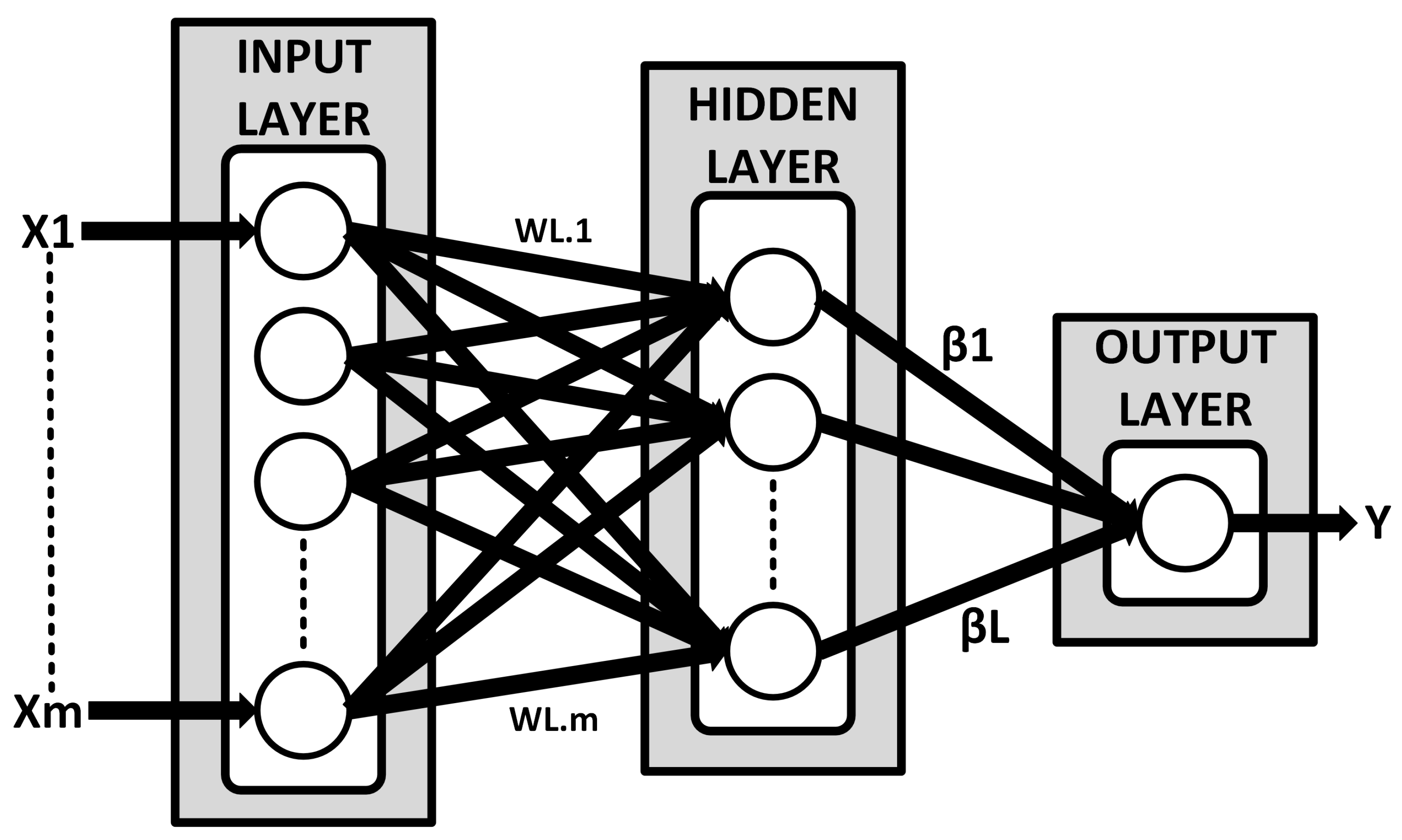
The architecture in Figure 3 is divided into three parts: the input layer $(x_1,x_2,\dots ,x_m)$, which is where the actual RTT values used as training data for building the RELM model are fed; and the input weights $(W_{L.1},\dots ,W_{L.m})$, which are randomly selected. Then there is the Hidden Layer, which is the core of RELM itself; its size is a parameter that is determined to create an optimal model. Next, there is $({\beta }_{L.1},\dots ,{\mathit{beta}}_{L.m})$, which represents the output weights that connect the hidden layer to the output layer.

Furthermore, the mathematical equation of RELM is almost the same as the ELM described previously; the only difference is the regularization constant on the output weights $\beta$ [42]. The mathematical equation is as follows:

$$\beta ={\left({\displaystyle \frac{1}{C}}+H^{T}H\right)}^{-1}{H}^T·y$$

(7)

It can be observed that for the RELM $\beta$, an additional regularization constant (C) is present. There is no iteration in RELM, as it is obtained analytically through Equation (7). In addition to mitigating overfitting, C enhances the model’s generalization performance, enabling it to adapt to new datasets. The selection of the regularization constant is still conducted through trial and error [44]. By comparing several values of the C parameter, the optimal result can be achieved.

In this study, the regularization constant C was initially selected using a trial-and-error procedure by evaluating values spaced by one decade (multiples of 10) over a wide range $({10}^{-12}$ to ${10}^{12})$ to identify an adequate setting. To further assess robustness and reduce the risk of overfitting, we evaluated the model using both a hold-out validation split and 5-fold cross-validation, which provides multiple train–validation partitions and reduces variance in the reported performance.

To improve reproducibility and avoid repeated manual reruns, we next implemented a brute-force decade-grid search within a predefined range. This approach evaluates all candidate C values in the specified interval and selects the best C* based on validation RMSE. While this is more systematic than manual trial-and-error, it remains sensitive to the choice of search bounds: if the optimal value lies outside the predefined range, the procedure returns the best value within the range rather than the global optimum.

To address this limitation, we propose an adaptive greedy heuristic for selecting C on a logarithmic scale. Instead of requiring fixed lower and upper bounds, the procedure starts from $C_0={10}^0$ (i.e., $C_0=1$) and explores both directions by evaluating $C_{Forward}=C\times 10$ and $C_{\mathrm{backward}}=C/10$. At each step, the candidate that yields the lowest validation RMSE is retained.

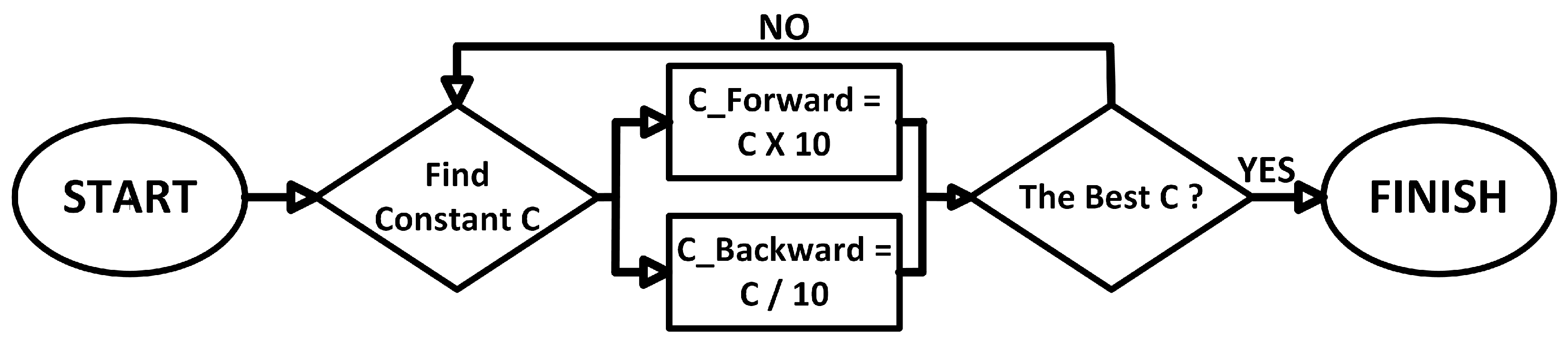
As illustrated in Figure 4, the search terminates using a tolerance-based stopping rule. Specifically, if the improvement in the validation RMSE relative to the best-so-far value is smaller than $ϵ=0.0001$ for $p=5$ consecutive iterations in both the forward and backward searches, the procedure stops to avoid unnecessary computations and returns the best C* found.

Algorithm 1 summarizes the proposed adaptive procedure for selecting the regularization constant C. The algorithm takes the dataset $\mathcal{D}$ as input and starts from an initial value $C_0$ (set to 1 in our experiments). At each iteration, the algorithm evaluates candidate values in a logarithmic step by exploring $C_{\mathrm{forward}}=C\times 10$ and $C_{\mathrm{backward}}=C/10$, and records the best validation RMSE, denoted as RMSE*, along with its corresponding C*.

The proposed procedure is an adaptive greedy heuristic on a logarithmic scale. At each iteration, it evaluates C values one decade above and below the current candidate ($C\times 10$ and $C/10$) and keeps the value that yields the lowest validation RMSE. The search stops when the RMSE improvement is smaller than $ϵ$ for p consecutive iterations, which removes the need to predefine fixed lower and upper bounds as required by brute-force grid search.

Algorithm 1 Adaptive log-step heuristic for selecting RELM regularization constant C (greedy decade search)

1:   Input: $H_{tr}, y_{tr}, H_{val}, y_{val}$      ▹ training/validation hidden matrices and targets

2:   Parameters: initial $C_0$, tolerance $ϵ$, patience p

3:   Output: selected C*

4:   function EvalRelm(C)

5:         $\beta \left(C\right)\leftarrow {\left({\displaystyle \frac{1}{C}}I+H_{tr}^T{H}_{tr}\right)}^{-1}{H}_{tr}^T{y}_{tr}$               ▹ RELM closed-form

6:         ${\widehat{y}}_{val}\left(C\right)\leftarrow H_{val}\beta \left(C\right)$

7:         $RMSE\left(C\right)\leftarrow \sqrt{{\displaystyle \frac{1}{n}}{\sum }_{i=1}^n{\left(y_{val,i}-{\widehat{y}}_{val,i}\left(C\right)\right)}^2}$

8:         return RMSE(C)

9:   end function

10: function SelectC($C_0,ϵ,p$)

11:         C* $\leftarrow C_0$

12:         RMSE* ← EvalRelm($C_0$)

13:         $C_{\uparrow }\leftarrow C_0,C_{\downarrow }\leftarrow C_0$

14:         $k_{\uparrow }\leftarrow 0,k_{\downarrow }\leftarrow 0$

15:         while $k_{\uparrow }<p$ or $k_{\downarrow }<p$ do

16:            if $k_{\uparrow }<p$ then

17:              $C_{\uparrow }\leftarrow 10\times C_{\uparrow }$

18:              $RMS{E}_{\uparrow }\leftarrow$EvalRelm($C_{\uparrow }$)

19:              if RMSE* $-RMS{E}_{\uparrow }>ϵ$ then

20:                   RMSE* $\leftarrow RMS{E}_{\uparrow },C*\leftarrow C_{\uparrow },k_{\uparrow }\leftarrow 0$

21:              else

22:                   $k_{\uparrow }\leftarrow k_{\uparrow }+1$

23:              end if

24:            end if

25:            if $k_{\downarrow }<p$ then

26:              $C_{\downarrow }\leftarrow C_{\downarrow }/10$

27:              $RMS{E}_{\downarrow }\leftarrow$EvalRelm($C_{\downarrow }$)

28:              if RMSE* $-RMS{E}_{\downarrow }>ϵ$ then

29:                    RMSE* $\leftarrow RMS{E}_{\downarrow },C^{*}\leftarrow C_{\downarrow },k_{\downarrow }\leftarrow 0$

30:              else

31:                   $k_{\downarrow }\leftarrow k_{\downarrow }+1$

32:              end if

33:            end if

34:         end while

35:         return C*

36: end function

3.3. Estimated RTT and Performance Evaluation

After building a model from the training data, it was tested on the validation data to assess overfitting. The model was used to determine the optimal $C_{value}$ using the built-in function, and subsequent evaluations utilizing the test data were conducted to assess the model’s performance. This step is critical because it integrates the core contribution of this research—an adaptive function that optimizes regularization, significantly improving RELM performance in dynamic environments.

Evaluation is performed to assess the performance of the constructed method using metrics such as MAE, RMSE, MAPE, and $R^2$. Performance evaluation is conducted using validation data for model selection and hyperparameter tuning. The test set is used strictly for final evaluation only and is never used for re-tuning. If performance is unsatisfactory during development, re-tuning is performed based on validation results (or cross-validation within the training set), not on the test set. However, if the model’s expected value is close to the actual value, the model is successful in this study [45].

The RTT variations generated via controlled delay injections and traffic bursts approximate several phenomena commonly observed in operational networks (e.g., congestion and queuing delay) under controlled settings but do not fully capture other dynamics such as packet loss, jitter variability, and routing/path changes. This provides an initial indication of feasibility in a controlled simulation environment; however, deployment-level feasibility should be further assessed using real-network traces/measurements that include loss, jitter, and path variability.

To assess the suitability and efficacy of the proposed function in terms of time and accuracy, we compared it with several alternative machine learning models, including the RELM model that used the same function. The objective of this scenario was to determine whether the model could serve as a more robust and reliable alternative to existing algorithmic models. A comparative evaluation focused on RMSE, MAE, MAPE, $R^2$, and training time to assess both accuracy and computational efficiency, key indicators in real-time RTT estimation.

After comparing several machine learning models, a comparison with existing research was conducted to ensure that the proposed function model is more reliable than existing research. This comparison highlights that, unlike most existing methods, which rely on static configurations or trial-and-error regularization, the proposed model achieves dynamic adaptation, resulting in superior generalization across diverse conditions and producing competitive performance metrics.

Following a comparison with other models, the proposed model was also applied to estimate other problems. The datasets were obtained from the “UC Irvine Machine Learning Repository” and used to evaluate the proposed model’s ability to solve various regression problems beyond the original RTT estimation task. This was done to ensure that the model was only suitable for the concern raised in this study, or whether it could also overcome several other problems. These regression tasks validate the robustness and transferability of the proposed model architecture beyond RTT estimation, indicating a sound methodological foundation.

4. Presentation, Analysis and Interpretation of Data

4.1. Data Presentation and Experiment Analysis

This chapter presents the experimental results of RTT estimation using RELM, which is tested on the activation function. It then discusses the selection of the regularization constant C, performed by brute force and using the proposed function. Then, the proposed function is compared with several machine learning models built and with those from existing research. Finally, the proposed function is implemented for several regression problems from the “UC Irvine Machine Learning Repository.”

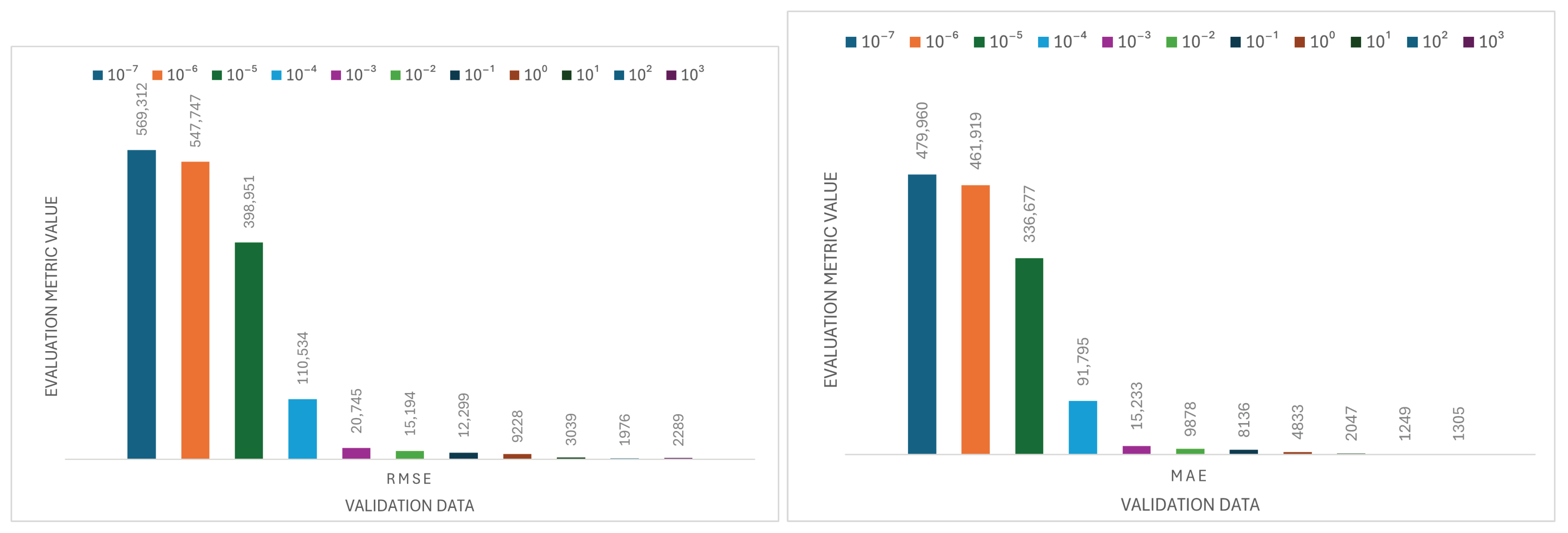
The accuracy results remain unchanged within the range of ${10}^{-12}$ to ${10}^{-8}$ and ${10}^4$ to ${10}^{12}$, so the data plot is omitted. Figure 5 illustrates the C constant data, with a range of ${10}^{-7}$ to ${10}^3$, which is displayed more clearly to show the accuracy values for RMSE and MAE.

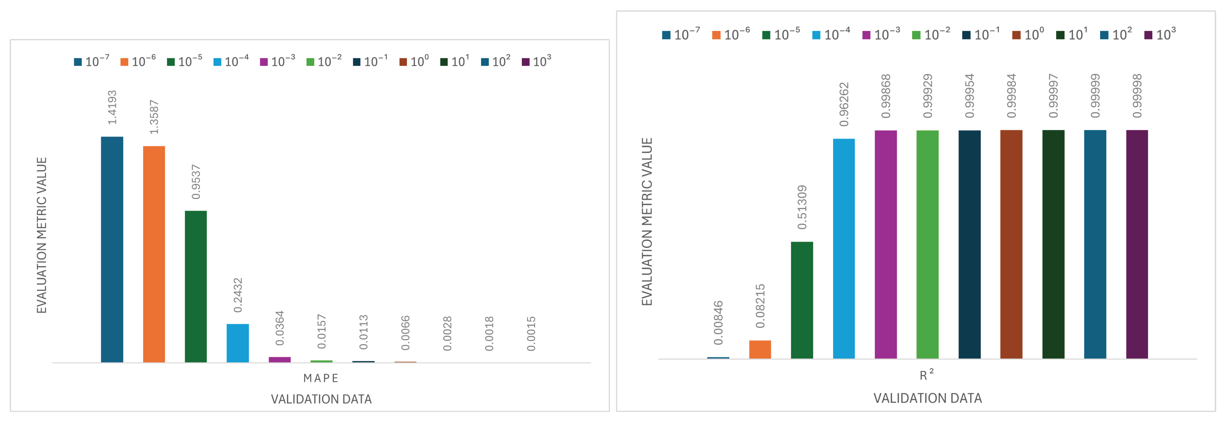
Figure 5 illustrates the accuracy of error values using MAE and RMSE on both validation and test data. The diagram shows that the best RMSE is achieved at $C={10}^2$. Figure 6 then depicts the accuracy of MAPE and $R^2$ errors within the same range.

Figure 6 shows that by using the ReLU activation function, the regularization constant is changed from ${10}^{-12}$ to ${10}^{12}$. In addition, to achieve the highest accuracy, this study selected $C={10}^2$ with the ReLU activation function. It used a hidden layer size of 150 as the optimal parameter, based on the lowest RMSE value. However, the above experiments were conducted through trial and error and took considerable time. Each time C was changed, the program should be run, and the resulting error accuracy noted, so it would take quite a long time if done one at a time. Because the regularization constant was changed from ${10}^{-12}$ to ${10}^{12}$, the trial-and-error time was less noticeable. However, if the regularization constant were adjusted from ${10}^{-50}$ to ${10}^{50}$, it would raise questions about its impact on the model’s performance. Therefore, in the future, an algorithm was suggested to select this $C_{value}$.

To ensure that the model was not too adaptive to the training set to produce a high accuracy value. The experiments were conducted using cross-validation on the previously best hidden layer, and execution time was also displayed to observe the program’s performance, as shown in

Table 1. Cross-validation results with k-fold = 5 and execution time for the best parameters.

Activation Function	RELM
	Metrics	150 Hidden Layer (C = 102)
Cross Validation (ReLU)	MAE	1092.72
	RMSE	2171.21
	MAPE	0.0017
	R2	0.9999
Execution Time (s)		0.0037216

. The cross-validation results are expressed as mean ± standard deviation across the 5 folds to demonstrate stability and reduce the risk of optimistic estimates from a single split.

Furthermore, in terms of error accuracy and execution time, Hidden Layer 150 has the fastest execution time. Additionally, after experimenting with cross-validation, the accuracy displayed is relatively optimal. The optimal parameters after the experiment are a hidden layer size of 150 and a $C_{value}={10}^2$, using ReLU as the activation function.

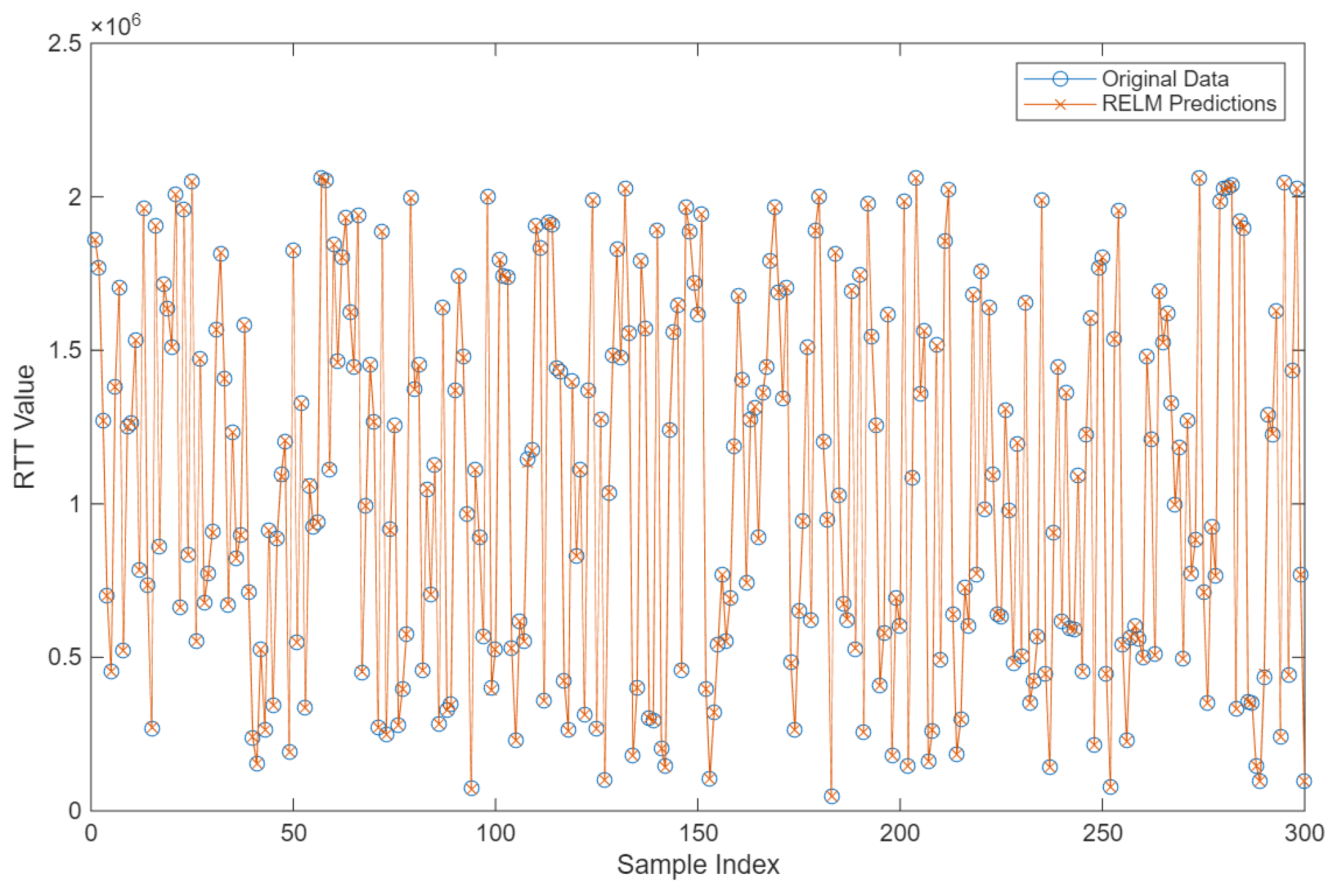
The results of the model against the test data are shown in a line plot graph in Figure 7. To improve the RELM algorithm, experiments were conducted by implementing a brute-force approach to determine the value of the constant C in the RELM model. The advantage of this enhanced RELM was that the algorithm only performed the best search using validation data, thereby reducing execution time. By limiting the value of C from ${10}^{-12}$ to ${10}^{12}$, the algorithm searched for the value of C within the specified range using the brute force approach.

This study focused on the program’s execution time.

Table 2. RELM for the best constant C using brute force.

Activation Function	RELM (Brute Force)
	Dataset	Execution Time (s)
ReLU Activation	Training Time	0.0053527
	Validation Time	0.025307
	Testing Time	0.0079633

illustrates the program execution time when using brute force as a constant selection. For the accuracy value, using brute-force search, the optimal $C_{value}$ was found to be ${10}^2$ through trial and error. The difference was that at this moment, upper and lower limits were provided to determine the value of the constant C. However, there was a weakness in this function: if $C={10}^{-12}$ to $C={10}^{12}$, there was no optimal value. In this case, the program generated the best value of C within that range, even if it was not the optimal one.

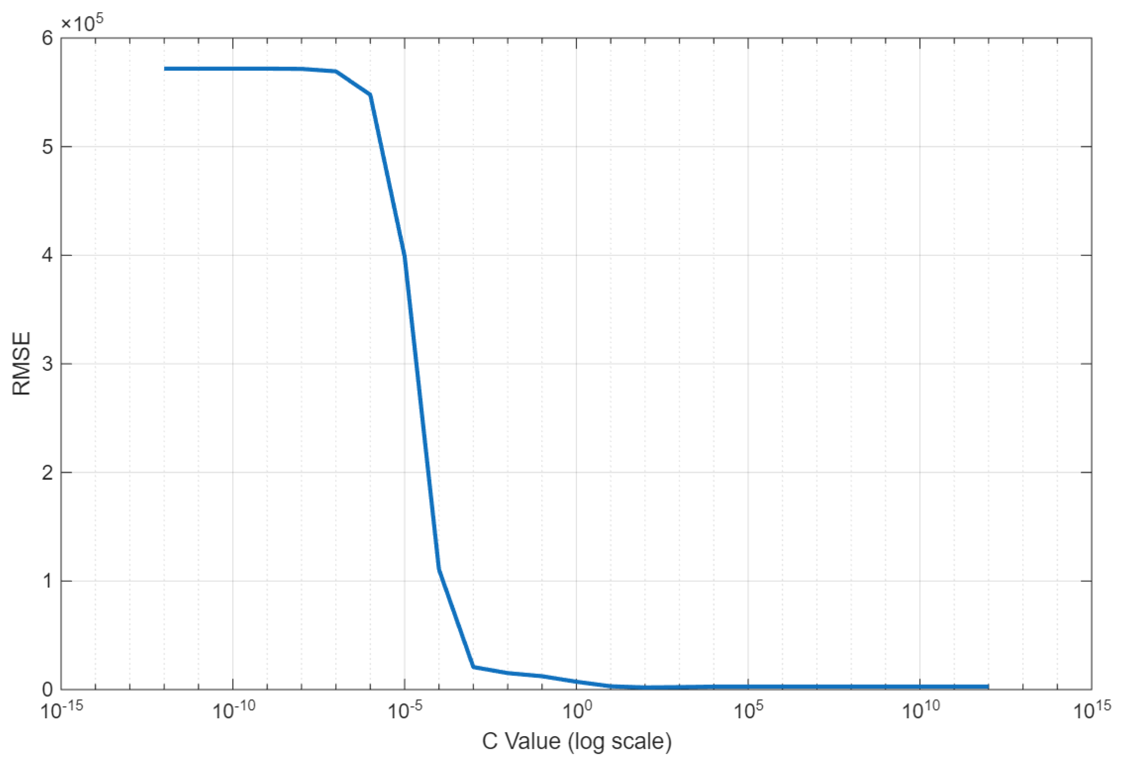
Figure 8 shows the graph of the $C_{value}$, based on the RMSE accuracy. To solve this problem, if no optimal value existed within this range, a function was created using the previously described tolerance limit. The initial value of C was set to $C={10}^0$. Then, it was divided into two parts: $C_{forward}=C\times 10$ when C was increasing, and $C_{backward}=C/10$ when C was decreasing.

Table 3. Enhanced RELM for the best constant C using the proposed function.

Activation Function	RELM (Proposed Function)
	Dataset	Execution Time (s)
ReLU Activation	Training Time	0.0034197
	Validation Time	0.014457
	Testing Time	0.0014153

gives the program execution time. The execution time is longer than that of brute force. If C were decreasing, the algorithm would have run only to $C={10}^{-5}$ because the accuracy remained the same or worsened after five consecutive backward iterations; therefore, it stopped at ${10}^{-5}$ for $C_{Backward}$. If C was increasing, even when finding the best accuracy at $C={10}^2$, the algorithm still ran forward to ${10}^7$. However, the accuracy was worse when five iterations were performed in reverse after finding the best accuracy, so $C_{Forward}$ was stopped at ${10}^7$. Examining the iterations, brute force performed 25 iterations from ${10}^{-12}$ to ${10}^{12}$, whereas the proposed function performed only 13 iterations from ${10}^{-5}$ to $C={10}^7$. Therefore, it can optimize the RELM algorithm without the need for trial-and-error to find the regularization constant.

Applying the results of the previous experiments, the proposed RELM was configured with 150 hidden neurons, the ReLU activation function, and the selected regularization constant $C={10}^2$. To ensure a fair comparison, all baseline models were evaluated under the same data split and preprocessing pipeline (standardization of X using training statistics only and normalization of Y using training statistics only, followed by de-normalization for reporting metrics). We compared the proposed method against several regression baselines, including Support Vector Regression (SVR), Generalized Additive Model (GAM), Decision Tree Regression, k-Nearest Neighbors (KNN), Random Forest, Gradient Boosted Decision Trees (GBDT), and Extreme Learning Machine (ELM).

Table 4. Comparison of regression performance and execution time under the unified (fair) evaluation pipeline.

Machine Learning	Validation				Testing				Execution Time (s)
	RMSE	MAE	MAPE	R2	RMSE	MAE	MAPE	R2	Train/Tune	Validation	Testing
SVR (RBF)	189,887.0361	134,397.1100	0.25965	0.88969	135,471.9927	97,581.8956	0.21816	0.95012	1.4607	0.026402	0.0062509
GAM (fitrgam)	31,599.1600	17,675.2620	0.0316960	0.99695	18,281.1355	12,170.7907	0.0209880	0.99909	272.3918	0.089907	0.091772
Decision Tree Regression	15,703.6146	10,862.3396	0.0231320	0.99925	13,447.5219	9129.2198	0.0157440	0.99951	1.4642	0.0025308	0.0005834
KNN Regression	15,975.8136	10,475.0000	0.0140710	0.99922	12,164.4453	9081.2133	0.0142630	0.99960	9.4485	0.011448	0.037323
Random Forest (TreeBagger)	10,682.5614	7692.0919	0.0135390	0.99965	9199.3896	6789.7109	0.0122830	0.99977	47.2547	0.014903	0.019242
GBDT (LSBoost, XGBoost-like)	6038.0116	4364.4292	0.0077504	0.9998884690	6140.5707	4418.3737	0.0081372	0.9998975117	123.5411	0.035009	0.040067
ELM (ReLU, 150 hidden)	2815.4728	1394.5745	0.0021684	0.99998	2705.2773	1194.6956	0.0016642	0.99998	0.12261	0.0092333	0.0047379
Enhanced RELM (Proposed, $C=100$)	1976.8061	1249.2079	0.0018148	0.99999	1589.6400	966.0401	0.0018184	0.99999	0.0034197	0.014457	0.0014153

summarizes the predictive performance and execution time results.

Overall, the proposed Enhanced RELM achieves consistently low error across both validation and testing sets while maintaining very low computational cost. Notably, its inference time is among the fastest, which is important for practical RTT estimation systems that require near real-time predictions.

Furthermore, this study compares different strategies for selecting the RELM regularization constant C. The first strategy is a trial-and-error approach, where C is manually adjusted across repeated runs to obtain a satisfactory result; although it can be quick for a single run, it is not systematic and may require many attempts. The second strategy is a brute-force grid search over a predefined range (e.g., ${10}^{-12}$ to ${10}^{12}$), which requires 25 evaluations to identify the best value within the grid; however, if the optimal C lies outside the chosen range, the method returns only the best value within the grid.

In contrast, the proposed adaptive search function does not require preset upper and lower bounds. It iteratively expands or contracts C (by a factor of 10) and stops based on a tolerance criterion, reducing unnecessary evaluations when improvements become marginal. In our experiments, the adaptive search explored approximately ${10}^{-5}$ to ${10}^7$ and required only 12 evaluations to reach the selected C value, resulting in a more efficient selection process than brute-force search while preserving strong predictive performance.

4.2. Real-World Evaluation Using Public WiFi RSS–RTT Dataset

While the preceding experiments demonstrate the effectiveness of the proposed Enhanced RELM under a controlled simulation environment, real-world wireless networks exhibit substantially different characteristics, including non-line-of-sight (NLOS) propagation, severe multipath effects, intermittent signal loss, and measurement noise that cannot be fully captured by synthetic datasets. To further assess the robustness and practical applicability of the proposed method, an additional evaluation was conducted using a publicly available real-world WiFi RSS–RTT dataset published by Feng et al. [46].

The dataset consists of three indoor deployment scenarios with distinct propagation conditions: a lecture theatre environment with entirely line-of-sight (LOS) links, an office environment with mixed LOS and NLOS conditions, and a corridor environment dominated by NLOS propagation. WiFi RTT and RSS measurements were collected using Google WiFi routers and a Google Pixel 3 smartphone, with ground-truth spatial coordinates obtained via grid-based reference-point labeling. Invalid RTT measurements (100,000 mm) and RSS values (−200 dBm), indicating missing or inaudible signals, were filtered prior to model training and evaluation.

For each scenario, the access point (AP) with the most valid RTT samples in the test set was automatically selected as the prediction target to ensure sufficient data support. The remaining RTT measurements from other APs, together with RSS values from all APs, were used as input features. To maintain fairness and consistency with the simulation-based experiments, the same standardized evaluation pipeline was applied: features were standardized using only training-set statistics, target RTT values were normalized during training and denormalized for metric reporting, and the proposed adaptive regularization-constant selection was performed exclusively on the validation set.

Table 5. Real-world RTT prediction performance across different indoor propagation scenarios.

Scenario	Propagation	RMSE (m)	MAE (m)	${\mathit{R}}^2$
Lecture Theatre	LOS	≈1.06	≈0.76	0.78
Office	Mixed LOS/NLOS	≈1.54	≈1.27	0.91
Corridor	Dominant NLOS	≈10.3	≈9.07	0.00

summarizes the predictive performance of the proposed Enhanced RELM across the three real-world scenarios. In the lecture theatre environment, where LOS propagation is stable, the proposed method achieves near-meter accuracy, indicating that the learned mapping remains informative under practical measurement noise. In the office environment, where mixed LOS/NLOS conditions are present, the accuracy degrades moderately but remains reliable, reflecting partial obstruction and multipath effects. In contrast, the corridor environment, dominated by NLOS propagation and severe multipath, exhibits substantially higher prediction errors and near-zero $R^2$ values, indicating that RTT measurements in such conditions are weakly correlated with spatial distance.

These results show that the observed performance degradation in NLOS-dominated environments is primarily driven by the physical characteristics of the wireless channel rather than the model’s learning capacity. Importantly, the proposed Enhanced RELM demonstrates consistent and realistic behavior across diverse propagation conditions, avoiding overly optimistic performance estimates and reinforcing the validity of the evaluation protocol.

We note that this dataset contains IEEE 802.11 mc WiFi RTT measurements (often used for ranging/positioning) rather than TCP RTT from transport sessions. Therefore, this experiment is reported as an out-of-domain robustness check, not as direct evidence that the model generalizes to operational TCP networks.

4.3. Discussion

Several studies, such as those by Subramanya et al. [37], have attempted to illustrate network bottlenecks by simulating a dumbbell topology, while other works, such as Jacobsson et al. [47], constructed network datasets to estimate RTT using features including queue state and link delay. In a similar spirit, this study develops a custom-built RTT dataset by simulating a dumbbell network topology across a broad range of delays in a controlled environment. This design enables systematic benchmarking and precise control over RTT variability, while acknowledging that certain real-world effects, such as packet loss, jitter, and dynamic routing changes, are not fully captured in simulation.

The near-perfect $R^2$ values observed in the simulation-based experiments should therefore be interpreted in the context of this controlled environment. Since RTT dynamics are generated under systematic delay configurations with limited uncontrolled noise sources, the resulting input–output relationship is highly structured. When strict leakage-prevention and validation protocols are applied, such conditions can naturally yield very high $R^2$ values. This behavior does not indicate overfitting but rather reflects the deterministic nature of the simulated setting.

To examine whether the proposed approach remains valid beyond this controlled scenario, an additional evaluation was conducted using a publicly available real-world WiFi RSS–RTT dataset with diverse propagation characteristics, including line-of-sight (LOS), mixed LOS/NLOS, and dominant NLOS environments. The results reveal a clear dependence of performance on the underlying wireless propagation conditions. In LOS-dominated environments, the proposed Enhanced RELM achieves near-meter accuracy, demonstrating that the learned mapping remains informative under practical measurement noise. In mixed LOS/NLOS scenarios, the performance degrades moderately but remains reliable. In contrast, in corridor environments dominated by NLOS propagation, the prediction accuracy deteriorates significantly, with high RMSE values and near-zero $R^2$. This outcome is consistent with the known instability of WiFi RTT measurements under severe multipath and obstruction, indicating that the primary limitation arises from the physical characteristics of the wireless channel rather than the model’s learning capacity.

Jordaan et al. [48] highlighted that the regularization parameter C in RELM plays a critical role in balancing model complexity and prediction error. Similarly, Li et al. [49] noted that identifying an optimal C value is challenging due to its interaction with other model factors. In this study, an adaptive heuristic was proposed to select the regularization constant on a logarithmic scale without requiring predefined upper and lower bounds. Experimental results demonstrate that the C value obtained using the proposed heuristic consistently yields high predictive accuracy with reduced execution time, effectively reducing the number of grid-search evaluations required.

Several studies have explored RTT prediction using machine learning techniques such as RNNs [9], LSTMs [25], hybrid neuro-fuzzy networks [28], adaptive filtering methods [27], and CNN-based models [29]. However, direct numerical comparison across prior studies is generally not strictly comparable due to differences in datasets, feature representations, and evaluation protocols. To mitigate this issue and enable a fair within-study comparison, representative baseline models from the literature were re-implemented and evaluated under the same experimental pipeline as the proposed method, including an identical train/validation/test split, training-only normalization, and validation-only hyperparameter selection. The results reported in

Table 6. Fair comparison under the same dataset and evaluation pipeline (60/10/30 split, training-only normalization, validation-only hyperparameter selection).

Method	RMSE	MAE	MAPE	${\mathit{R}}^2$	Train Time (s)	Test Time (s)
LSTM (Hagos et al. [25], re-impl.)	30,875.3672	24,929.7129	0.057901	0.99741	67.2832	0.019274
Hybrid Neuro-Fuzzy (Damaševičius et al. [28], ANFIS re-impl.)	1207.2281	664.7028	0.0013106	1.00000	539.9954	0.13683
Adaptive Filtering (Guodong et al. [27], NLMS re-impl.)	9484.7168	6901.1684	0.011241	0.99976	0.0010274	0.0001074
MDN-CNN (Mohammed et al. [29], re-impl.)	13,097.8683	9920.6364	0.013704	0.99953	38.152	0.38213
Gated RNN (Dong et al. [9], GRU as MGU-like re-impl.)	16,350.5781	10,970.5254	0.033721	0.99927	68.2072	0.036107
Proposed Enhanced RELM (fair pipeline)	1589.6400	966.0401	0.0018184	0.99999	0.0034197	0.0014153

Note: The results in Table 6 are obtained from our reimplementations under the same dataset and evaluation protocol and thus are intended for fair within-study comparison. Reported metrics from the original papers are not directly comparable due to differences in datasets and experimental settings.

demonstrate that the proposed Enhanced RELM achieves a favorable accuracy–efficiency trade-off on the considered simulation dataset.

Overall, the combined evidence from simulation-based and real-world evaluations indicates that the proposed Enhanced RELM provides reliable, computationally efficient RTT estimation under informative signal conditions. At the same time, the real-world experiments highlight the inherent limitations imposed by wireless propagation physics, particularly under NLOS conditions. Further validation on operational networks with dynamic traffic patterns, packet loss, and routing changes remains an important direction for future work.

• Limitations. The simulation-based evaluation uses a single dumbbell topology and a controlled delay-injection procedure; thus, the results do not generalize across different topologies, routing dynamics, packet-loss regimes, or highly variable traffic patterns. Extending the evaluation to multiple topologies and operational traces with loss/jitter/path changes is an important next step.

5. Conclusions

This study developed an optimized Regularized Extreme Learning Machine (RELM) by introducing an adaptive regularization-constant selection heuristic to improve both estimation accuracy and computational efficiency. Multiple experimental configurations were evaluated, including a grid search over activation functions (Sigmoid, ReLU, and Tanh) and three strategies for selecting the regularization constant C: manual trial-and-error, fixed-range brute-force search, and the proposed adaptive (dynamic) search function.

Experimental results on the simulation-based RTT dataset indicate that RELM configured with the ReLU activation function and a hidden-layer size of 150, and $C={10}^2$ achieves the best overall performance, yielding $R^2=0.9999$, $\mathrm{MAPE}=0.0018$, $\mathrm{MAE}=966.0401$, and $\mathrm{RMSE}=1589.64$ on the test set. Under a unified and fair evaluation pipeline, the proposed Enhanced RELM consistently outperformed the considered baseline regression models (SVR, GAM, Decision Tree, KNN, Random Forest, GBDT, and ELM) while maintaining very low computational cost, making it suitable for latency-sensitive RTT estimation tasks.

Beyond controlled simulations, the proposed method was further evaluated using a public real-world WiFi RSS–RTT dataset encompassing diverse indoor propagation conditions, including line-of-sight (LOS), mixed LOS/NLOS, and dominant NLOS environments. The real-world results demonstrate that the Enhanced RELM achieves near-meter accuracy in LOS and mixed propagation scenarios, while performance degrades substantially under dominant NLOS conditions. This behavior reflects the intrinsic limitations of WiFi RTT measurements under severe multipath and obstruction, rather than shortcomings of the learning model itself, and highlights the strong dependence of RTT estimation accuracy on physical channel characteristics.

In addition to accuracy gains, the proposed adaptive C-selection function provides a systematic and efficient alternative to manual tuning and brute-force search. By iteratively expanding or contracting C on a logarithmic scale and terminating based on a tolerance-driven criterion, the method reduces the number of required evaluations while preserving predictive performance. Overall, the proposed Enhanced RELM offers a favorable trade-off between accuracy and efficiency for RTT estimation in both controlled and real-world settings.

Nevertheless, while the present study includes evaluation on a public real-world dataset, further validation on operational networks with dynamic traffic patterns, packet loss, heterogeneous hardware, and routing/path variability remains an important direction for future work.

References

1. Mirkovic, D.; Armitage, G.; Branch, P. A survey of round trip time prediction systems. IEEE Commun. Surv. Tutor. 2018, 20, 1758–1776. [Google Scholar] [CrossRef]
2. Patil, H.; Sharma, K. Extreme learning machine: A comprehensive survey of theories & algorithms. In 2023 International Conference on Computational Intelligence and Sustainable Engineering Solutions (CISES), 2023; IEEE: Piscataway, NJ, USA, 2023; pp. 749–756. [Google Scholar] [CrossRef]
3. Huang, G.B.; Zhu, Q.Y.; Siew, C.K. Extreme learning machine: A new learning scheme of feedforward neural networks. In 2004 IEEE International Joint Conference on Neural Networks (IEEE Cat. No. 04CH37541); IEEE: Piscataway, NJ, USA, 2004; Volume 2, pp. 985–990. [Google Scholar] [CrossRef]
4. Martinsen, P.E.; Reddy, K.T.; Wing, D.; Singh, V. Measurement of Round-Trip Time and Fractional Loss Using Session Traversal Utilities for NAT (STUN). RFC 7982. 2016. Available online: https://www.rfc-editor.org/info/rfc7982 (accessed on 25 January 2025).
5. Huang, G.; Huang, G.B.; Song, S.; You, K. Trends in extreme learning machines: A review. Neural Netw. 2015, 61, 32–48. [Google Scholar] [CrossRef]
6. Sailellah, H.; Nuha, H.H. Round-Trip Time Estimation Using Regularized Extreme Learning Machine. In Proceedings of the 2024 International Conference on Artificial Intelligence, Blockchain, Cloud Computing, and Data Analytics (ICoABCD), Bali, Indonesia, 20–21 August 2024; pp. 79–84. [Google Scholar] [CrossRef]
7. Kalidindi, S.; Zekauskas, M.J.; Almes, D.G.T. A Round-trip Delay Metric for IPPM. RFC 2681. 1999. Available online: https://www.rfc-editor.org/info/rfc2681 (accessed on 20 March 2025).
8. Jacobsson, K.; Hjalmarsson, H.; Möller, N.; Johansson, K.H. Round trip time estimation in communication networks using adaptive kalman filtering. In Proceedings of the Reglermöte, Gothenburg, Sweden, 26–27 May 2004. [Google Scholar]
9. Dong, A.; Du, Z.; Yan, Z. Round trip time prediction using recurrent neural networks with minimal gated unit. IEEE Commun. Lett. 2019, 23, 584–587. [Google Scholar] [CrossRef]
10. Maiti, A.; Kist, A.A.; Maxwell, A.D. Estimation of round trip time in distributed real time system architectures. In 2013 Australasian Telecommunication Networks and Applications Conference (ATNAC); IEEE: Piscataway, NJ, USA, 2013; pp. 57–62. [Google Scholar] [CrossRef]
11. Goudru, N.; Puneeth, R.; Rao, K.P.N. Enhancement of Performance of Round-Trip Time Using Kalman Filtering. In Advances in VLSI, Signal Processing, Power Electronics, IoT, Communication and Embedded Systems: Select Proceedings of VSPICE 2020; Springer: Berlin/Heidelberg, Germany, 2021; pp. 99–108. [Google Scholar] [CrossRef]
12. Stadnik, W.; Nowak, Z. The impact of web pages’ load time on the conversion rate of an e-commerce platform. In International Conference on Information Systems Architecture and Technology; Springer: Berlin/Heidelberg, Germany, 2017; pp. 336–345. [Google Scholar]
13. Galletta, D.F.; Henry, R.; McCoy, S.; Polak, P. Web site delays: How tolerant are users? J. Assoc. Inf. Syst. 2004, 5, 1–28. [Google Scholar] [CrossRef]
14. Liborio Filho, J.D.M.; de Souza Coelho, M.; Melo, C.A. Super-resolution on edge computing for improved adaptive HTTP live streaming delivery. In 2021 IEEE 10th International Conference on Cloud Networking (CloudNet); IEEE: Piscataway, NJ, USA, 2021; pp. 104–110. [Google Scholar]
15. Laniewski, D.; Lanfer, E.; Aschenbruck, N. Measuring mobile Starlink performance: A comprehensive look. IEEE Open J. Commun. Soc. 2025, 6, 1266–1283. [Google Scholar] [CrossRef]
16. Kaseng, F.; Lezama, P.; Inquilla, R.; Rodriguez, C.R. Evolution and advance usage of Internet in Peru. 3C TIC Cuad. Desarro. Apl. TIC 2020, 9, 113–127. [Google Scholar] [CrossRef]
17. Chong, K.T.; Yoo, S.G. Neural network prediction model for a real-time data transmission. Neural Comput. Appl. 2006, 15, 373–382. [Google Scholar] [CrossRef]
18. Liu, X.; Zhou, Y.; Meng, W.; Luo, Q. Functional extreme learning machine for regression and classification. Math. Biosci. Eng. 2023, 20, 3768–3792. [Google Scholar] [CrossRef]
19. Wu, Q.; Wang, F.; An, Y.; Li, K. L1-Norm Robust Regularized Extreme Learning Machine with Asymmetric C-Loss for Regression. Axioms 2023, 12, 204. [Google Scholar] [CrossRef]
20. Das, P.; Nanda, S. An Improved Ridge Regression-Based Extreme Learning Machine for the Prediction of Diabetes. In International Conference on Communication, Circuits, and Systems: IC3S 2020; Springer: Berlin/Heidelberg, Germany, 2021; pp. 541–547. [Google Scholar] [CrossRef]
21. Yıldırım, H.; Özkale, M.R. An enhanced extreme learning machine based on Liu regression. Neural Process. Lett. 2020, 52, 421–442. [Google Scholar] [CrossRef]
22. Fan, Q.W.; He, X.S.; Yang, X.S. Smoothing regularized extreme learning machine. In International Conference on Engineering Applications of Neural Networks; Springer: Berlin/Heidelberg, Germany, 2018; pp. 83–93. [Google Scholar] [CrossRef]
23. Tang, Y.; Li, C. An Online Network Intrusion Detection Model Based on Improved Regularized Extreme Learning Machine. IEEE Access 2021, 9, 94826–94844. [Google Scholar] [CrossRef]
24. Dasgupta, B.; Valles, D.; McClellan, S. Estimating TCP RTT with LSTM Neural Networks. In Proceedings of the International Conference on Artificial Intelligence (ICAI). The Steering Committee of the World Congress in Computer Science, Computer Engineering and Applied Computing (WorldComp), Madrid, Spain, 6–9 November 2019. [Google Scholar]
25. Hagos, D.H.; Engelstad, P.E.; Yazid, A.; Griwodz, C. A Deep Learning Approach to Dynamic Passive RTT Prediction Model for TCP. In Proceedings of the 2019 IEEE 38th International Performance Computing and Communications Conference (IPCCC), London, UK, 29–31 October 2019; pp. 1–10. [Google Scholar] [CrossRef]
26. Arouche Nunes, B.A.; Veenstra, K.; Ballenthin, W.; Lukin, S.; Obraczka, K. A machine learning framework for TCP round-trip time estimation. EURASIP J. Wirel. Commun. Netw. 2014, 2014, 47. [Google Scholar] [CrossRef]
27. Li, G.; Zhao, N.; Liu, C. Round Trip Time estimation based on adaptive filtering. In 2009 First International Conference on Information Science and Engineering; IEEE: Piscataway, NJ, USA, 2009; pp. 1842–1846. [Google Scholar] [CrossRef]
28. Damaševičius, R.; Sidekerskiene, T. Short time prediction of cloud server round-trip time using a hybrid neuro-fuzzy network. J. Artif. Intell. Syst. 2020, 2, 133–148. [Google Scholar] [CrossRef][Green Version]
29. Mohammed, S.A.; Shirmohammadi, S.; Altamimi, S. Artificial Intelligence-Based Distributed Network Latency Measurement. In Proceedings of the 2019 IEEE International Instrumentation and Measurement Technology Conference (I2MTC), Auckland, New Zealand, 20–23 May 2019; pp. 1–6. [Google Scholar] [CrossRef]
30. Gu, Y.; Towsley, D.; Hollot, C.V.; Zhang, H. Congestion Control for Small Buffer High Speed Networks. In Proceedings of the IEEE INFOCOM 2007—26th IEEE International Conference on Computer Communications, Anchorage, AK, USA, 6–12 May 2007; pp. 1037–1045. [Google Scholar] [CrossRef]
31. Bigdeli, N.; Haeri, M. ARM-PFC an optimized AQM congestion controller in TCP/IP networks. Iran. J. Sci. Technol. Trans. B Eng. 2007, 31, 663. [Google Scholar]
32. Esmaeili, A.; Shakeri, E. Bacterial Foraging Optimization Robust-RED for AQM/TCP Network. Int. J. Model. Optim. 2011, 1, 49–55. [Google Scholar] [CrossRef]
33. Froldi, C.A.; da Fonseca, N.L.S.; Papotti, C.; Manzato, D.A.G. Performance evaluation of the DCCP protocol in high-speed networks. In 2010 15th IEEE International Workshop on Computer Aided Modeling, Analysis and Design of Communication Links and Networks (CAMAD) 2010; IEEE: Piscataway, NJ, USA, 2010; pp. 41–46. [Google Scholar] [CrossRef]
34. Tang, J.; Jiang, Y.; Dai, X.; Liang, X.; Fu, Y. TCP-WBQ: A backlog-queue-based congestion control mechanism for heterogeneous wireless networks. Sci. Rep. 2022, 12, 3419. [Google Scholar] [CrossRef] [PubMed]
35. DasGupta, B. Reducing TCP Retransmissions by Using Machine Learning for More Accurate RTT Estimation; Texas Digital Library: Austin, TX, USA, 2019. [Google Scholar]
36. Wang, Y.; Jiang, X.; Shi, Y. A Serpentine Meander Delay Line with dumbbell-shaped stub. In 2023 IEEE 11th Asia-Pacific Conference on Antennas and Propagation (APCAP); IEEE: Piscataway, NJ, USA, 2023; pp. 1–2. [Google Scholar] [CrossRef]
37. Subramanya, P.; Vinayaka, K.; Gururaj, H.; Ramesh, B. Performance evaluation of high speed TCP variants in dumbbell network. IOSR J. Comput. Eng. 2014, 16, 49–53. [Google Scholar] [CrossRef]
38. Mateen, A.; Zaman, M. Congestion Control Algorithms Evaluation of TCP Linux Variants in Dumbbell. J. Inst. Internet Broadcast. Commun. 2016, 16, 139–145. [Google Scholar] [CrossRef]
39. Huang, G.B.; Zhou, H.; Ding, X.; Zhang, R. Extreme learning machine for regression and multiclass classification. IEEE Trans. Syst. Man Cybern. Part B (Cybern.) 2011, 42, 513–529. [Google Scholar] [CrossRef]
40. Huang, G.B.; Zhu, Q.Y.; Siew, C.K. Extreme learning machine: Theory and applications. Neurocomputing 2006, 70, 489–501. [Google Scholar] [CrossRef]
41. Deng, W.; Zheng, Q.; Chen, L. Regularized extreme learning machine. In 2009 IEEE Symposium on Computational Intelligence and Data Mining; IEEE: Piscataway, NJ, USA, 2009; pp. 389–395. [Google Scholar] [CrossRef]
42. Nuha, H.; Mohandes, M.; Rehman, S.; A-Shaikhi, A. Vertical Wind Speed Extrapolation Using Regularized Extreme Learning Machine. FME Trans. 2022, 50, 413. [Google Scholar] [CrossRef]
43. Zhang, K.; Luo, M. Outlier-robust extreme learning machine for regression problems. Neurocomputing 2015, 151, 1519–1527. [Google Scholar] [CrossRef]
44. Id, I.D. Machine Learning: Teori, Studi Kasus dan Implementasi Menggunakan Python; Unri Press: Pekanbaru, Indonesia, 2021; Volume 1. [Google Scholar]
45. Saputra, I.; Kristiyanti, D.A. Machine Learning Untuk Pemula; Informatika: Redwood City, CA, USA, 2022. [Google Scholar]
46. Feng, X.; Nguyen, K.A.; Luo, Z. A WiFi RSS-RTT Indoor Positioning Model Based on Dynamic Model Switching Algorithm. IEEE J. Indoor Seamless Position. Navig. (J-ISPIN) 2024, 2, 151–165. [Google Scholar] [CrossRef]
47. Jacobsson, K.; Hjalmarsson, H.; Möller, N.; Johansson, K.H. Estimation of RTT and andwidth for congestion control applications in communication networks. In IEEE CDC, Paradise Island, Bahamas; IEEE: Piscataway, NJ, USA, 2004. [Google Scholar]
48. Jordaan, E.; Smits, G. Estimation of the regularization parameter for support vector regression. In 2002 International Joint Conference on Neural Networks. IJCNN’02 (Cat. No. 02CH37290); IEEE: Piscataway, NJ, USA, 2002; Volume 3, pp. 2192–2197. [Google Scholar]
49. Li, H.; Bai, L.; Gao, W.; Xie, J.; Huang, L. Many-objective coevolutionary learning algorithm with extreme learning machine auto-encoder for ensemble classifier of feedforward neural networks. Expert Syst. Appl. 2024, 246, 123186. [Google Scholar] [CrossRef]
Figure 1. Flowchart diagram of the system.
Network 06 00010 g001
Figure 2. Topology of the Dumbbell Architecture.
Network 06 00010 g002
Figure 3. The Architecture of the RELM.
Network 06 00010 g003
Figure 4. Flowchart of the proposed function.
Network 06 00010 g004
Figure 5. The Best C Constant from 10 7 to 10 3 (RMSE and MAE).
Network 06 00010 g005
Figure 6. The Best C Constant from 10 7 to 10 3 : MAPE and R 2 .
Network 06 00010 g006
Figure 7. Line Plot for Data Test.
Network 06 00010 g007
Figure 8. RMSE Accuracy Graph for Constant C.
Network 06 00010 g008