Modified Index Policies for Multi-Armed Bandits with Network-like Markovian Dependencies

Abstract

Sequential decision-making in dynamic and interconnected environments is a cornerstone of numerous applications, ranging from communication networks and finance to distributed blockchain systems and IoT frameworks. The multi-armed bandit (MAB) problem is a fundamental model in this domain that traditionally assumes independent and identically distributed (iid) rewards, which limits its effectiveness in capturing the inherent dependencies and state dynamics present in some real-world scenarios. In this paper, we lay a theoretical framework for a modified MAB model in which each arm’s reward is generated by a hidden Markov process. In our model, each arm undergoes Markov state transitions independent of play in a way that results in varying reward distributions and heightened uncertainty in reward observations. The number of states for each arm can be up to three states. A key challenge arises from the fact that the underlying states governing each arm’s rewards remain hidden at the time of selection. To address this, we adapt traditional index-based policies and develop a modified index approach tailored to accommodate Markovian transitions and enhance selection efficiency for our model. Our proposed proposed Markovian Upper Confidence Bound (MC-UCB) policy achieves logarithmic regret. Comparative analysis with the classical UCB algorithm reveals that MC-UCB consistently achieves approximately a 15% reduction in cumulative regret. This work provides significant theoretical insights and lays a robust foundation for future research aimed at optimizing decision-making processes in complex, networked systems with hidden state dependencies.

1. Introduction

Decision-making in environments with network-like dependencies presents a fundamental challenge across various fields, including communication networks, finance, and complex distributed systems [1,2,3,4]. In such environments, a decision-maker faces interconnected structures where actions taken on one element may influence the states or rewards of others, thereby creating dynamic dependencies reminiscent of those found in networked systems. Examples of such networks can be found in resource allocation across multiple communication channels in IoT (Internet of Things) sensor networks [5], throughput optimization in distributed blockchain ecosystems [6], adaptive QoS (Quality of Service) management in communication networks [7], and security or intrusion detection frameworks in large-scale system administration scenarios [8]. In these contexts, the multi-armed bandit (MAB) problem, where a player repeatedly selects among multiple uncertain options (arms), becomes more intricate due to underlying and often hidden state transitions that evolve over time.

The original classical MAB formulation, introduced by Robbins [9,10], assumes that each arm’s reward distribution remains fixed and independent over time. However, in networked scenarios, these assumptions rarely hold: the reward distributions may shift due to underlying Markovian state transitions that are hidden from the decision-maker [11]. Arms in such a scenario can represent network nodes, communication links, or distributed resources whose performance and reliability evolve with time. The agent must continually learn and adapt, taking into account latent transitions that are reminiscent of evolving network conditions.

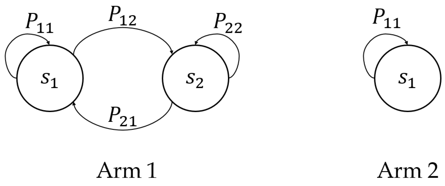
In this paper, we lay a theoretical framework for a modified MAB model in which each arm’s reward is generated by a hidden Markov process. This approach models the type of network-like dependencies found, for example, in dynamic IoT sensor networks—where channel conditions and sensor states change stochastically and are not directly observable, yet these state changes critically affect the rewards (e.g., reliable data transmission or efficient resource utilization). Each arm in our model can transition among up to three states, each associated with a different reward distribution, regardless of whether the arm is played. The result is a problem setting that demands sophisticated exploration–exploitation strategies that identify the best arms under evolving conditions and also cope with underlying dynamics that reflect network interdependencies.

In this context, we evaluate the decision-maker’s performance using the concept of regret, a metric that captures the cost of uncertainty in networked decision-making environments. Regret is defined as the difference between the expected reward an ideal policy—one with complete knowledge of all arm statistics or hindsight advantage—would achieve, and the reward achieved by the decision-maker’s actual strategy. An ideal policy would consistently select the arm yielding the highest expected reward over time. This concept, commonly referred to as weak regret, is a central performance measure in uncertain decision problems, as highlighted by Auer et al. [12]. Our study focuses on regret, particularly within interconnected, network-like settings.

MAB problems with Markovian rewards significantly heighten complexity due to dynamic dependencies that reflect networked interactions. Here, each arm is modeled as a Markov process with a finite set of states, each linked to a unique reward distribution. The transition between states follows a known probability matrix, introducing a memory element into the decision process where rewards depend not only on the current choice but also on the hidden state of each arm [13,14,15,16]. This Markovian structure effectively simulates a network in which states and rewards are dynamically interdependent over time.

The state transitions are determined by predefined probabilities, yet the exact state of each arm remains hidden. This creates a layer of opacity similar to unobserved interactions in networked systems [17,18,19]. Consequently, the player must infer each arm’s state from the history of observed rewards. This amplifies the challenge of the exploration–exploitation trade-off. The decision-maker faces a networked challenge: to exploit high-reward arms based on historical performance or to explore underused arms to reveal potential reward structures. Figure 1 illustrates an example of the problem and highlights the network-like dependencies across arms.

A core challenge in this interconnected framework is to develop strategies that effectively balance immediate rewards with potential future gains that could arise from transitioning into more advantageous states [20,21]. This networked trade-off between short-term exploitation and long-term exploration is not purely theoretical or network-related; it mirrors complex, real-world decision-making environments such as financial portfolio management or adaptive clinical trials where treatments impact outcomes over time [22,23,24,25].

In this work, we address these challenges by introducing a novel theoretical approach to the MAB problem with Markovian dynamics and network-like dependencies where each arm has up to three possible states. We adapt traditional index policies to account for the intricate structure of state transitions. Our focus is on refining these policies to achieve robust performance by attaining logarithmic regret even within the complex networked dynamics of hidden state transitions. We further compare our modified index-based policies with the classic upper confidence bound (UCB) algorithm. This study thus sets the stage for a deeper understanding of decision strategies within networked environments involving uncertainty and dynamic dependencies.

1.1. Main Findings

This paper makes the following theoretical contributions:

• We demonstrate that for each arm, represented as an irreducible, finite-state, aperiodic, and reversible three-state Markov chain, simple sample mean-based index policies can achieve logarithmic regret uniformly over time, even in interconnected settings resembling networked dependencies.
• We simplify the analysis of state transition probabilities by modeling the arms as Markov chains with identical rewards that capture basic network-like structures in which transitions are dependent on state dynamics.
• We present a numerical comparison of the regret incurred by our sample mean-based index policy and evaluate its performance relative to other policies.

1.2. Application Context and Conceptual Validation in Network-like Scenarios

While our primary contribution is theoretical, it is helpful to illustrate how this framework can be built on to conceptually extend to real network scenarios. Consider, for example, the following contexts:

• Security [26]: Arms may represent intrusion detection strategies whose efficacy varies as an adversary’s tactics evolve over time. Each state transition corresponds to a shift in the threat environment. Our Markovian MAB framework can guide strategic decisions to maintain robust defense while learning dynamically about evolving threats.
• Distributed Blockchain Systems [27]: Nodes or shards in a blockchain network might yield variable validation rewards depending on their state of congestion or consensus participation. The Markovian structure models the dynamic nature of node availability and network conditions in a way that would help a node operator choose where to allocate resources or which shard to support over time.
• QoS in Communication Networks [7]: Network links may fluctuate between high-quality, moderate, and poor states due to changing traffic patterns. By representing each link as a Markovian arm, our framework can assist in selecting the best channel at any given time in order to balance the exploration of uncertain but potentially high-quality links with the exploitation of known reliable ones.
• IoT and System Administration [28]: IoT nodes or servers can transition between states that reflect varying processing loads or energy conditions. The Markovian MAB model helps a controller decide which node to query or utilize for computations, thereby maximizing long-term performance.

In sum, while this work is focused on the theoretical aspects and fundamental results for up to three states, it offers a roadmap for future empirical explorations and practical implementations. The stylized simulation experiments that we show later serve as a preliminary demonstration and show that the theoretical principles hold in a controlled synthetic environment, thus setting the stage for subsequent research aiming at more comprehensive benchmarking in real-world network contexts.

The remainder of the paper is structured as follows. Section 2 gives the related work. Section 3 presents the preliminaries. Section 4 shows the problem formulation. The index policy and its regret analysis are given in Section 5. Section 6 shows our numerical simulation results, and finally, Section 7 concludes the paper.

2. Related Work

The literature on the MAB problem is vast and has evolved considerably from the original formulations focusing on independent and identically distributed (iid) reward processes. Early seminal work by Robbins and Lai  [9,10] established foundations for the iid case for certain known environments. Over time, researchers have explored a broad spectrum of MAB extensions that incorporate various forms of structure and dynamics. Notably, Markovian reward processes represent a key generalization and enable the modeling of scenarios where arm states—and thus rewards—evolve with memory and dependence on previous states.

Early explorations into Markovian bandits can be found in the work of Anantharam et al. [29], which analyzed index policies effective for arms governed by irreducible, finite-state, aperiodic Markov chains. Their approach demonstrated how arms with state-dependent rewards could still be tackled through index strategies that generalize the Gittins index concept [30]. While these studies set important precedents for handling Markovian structures, they often made simplifying assumptions, such as a single-parameter transition function or identical state spaces across arms. In contrast, our framework does not presume a single-parameter form for transition probabilities, nor does it require identical state spaces. By allowing each arm to transition among up to three states under distinct probability kernels, we offer a more flexible setting that can model diverse types of network dependencies.

Building upon this foundation, research has examined the problem of achieving low regret under more general conditions. Agrawal [31] and Auer et al. [32] established classical logarithmic regret results for iid settings. Their contributions included index and UCB-based strategies that guarantee optimal asymptotic and even uniformly logarithmic performance over time. They rely heavily on the iid assumption and do not directly address the complexities introduced by state transitions or network-like interdependencies. More recent works have begun to relax these assumptions. For instance, Garivier and Moulines [33] and Besbes et al. [34] considered bandit problems with non-stationary reward distributions in a way that captures some aspects of temporal dynamics without fully embracing Markovian state dependence. Such approaches typically rely on “resetting” or “sliding-window” techniques that do not directly exploit known Markovian transition structures.

In parallel, other authors have studied scenarios where multiple users or decision-makers interact with the same set of arms in network settings, leading to complex dynamics and collisions among players [35,36,37]. Here, the challenge lies in coordinating multiple agents to minimize interference and collectively achieve low regret. While such multi-player frameworks mirror network complexity, their primary focus is on handling concurrency and competition rather than modeling state evolution within each arm. Our approach differs by focusing explicitly on Markovian transitions at the arm level rather than strategic interactions among multiple decision-makers.

The distinction between rested and restless bandits further highlights the complexity in Markovian settings. In classical rested bandits, the state of an unplayed arm remains frozen until chosen again, as examined in works like those of Ortner [38] and Raj and Kalyani [39]. However, in restless bandits, arm states evolve regardless of selection, making the problem significantly more complex. The restless bandits formualation has explored structural results and approximation algorithms for special cases [11,40]. Our framework takes a step forward by considering a setting in which all arms transition at every round, falling somewhere between the fully rested and fully restless extremes, and by establishing logarithmic regret bounds in this intermediate regime.

Compared to the closely related studies such as [15,29], our work introduces a novel solution. For instance, Tekin et al. [15] restrict attention to two-state arms with transitions occurring only when the arm is played, which simplifies the analysis but limits applicability. In [29], the reward-generating process is governed by a single parameter and identical state spaces across all arms. In contrast, our model allows each arm to have distinct state spaces and transition matrices, and does not rely on a single-parameter structure. We also require that the reward process be reversible, a mild assumption that enables cleaner theoretical analysis. The indices we derive rely on sample means rather than complicated recursive computations, and yield uniform logarithmic regret bounds rather than merely asymptotic guarantees.

Lastly, recent theoretical studies on bandits with structure—such as Liu et al. [41], who considered bandits with feedback graphs, or Chen et al. [42], who looked at dynamic networked scenarios—point to a growing interest in incorporating more nuanced dependencies into MAB models. Our results add to this literature by providing a more direct handle on Markovian state transitions within a theoretically grounded bandit framework.

In sum, our work occupies a unique position at the intersection of Markovian bandits, structured bandit problems, and theoretical analyses that strive for uniform logarithmic regret. While prior research established important groundwork in various specialized settings, we advance the state of the art by offering a flexible, three-state Markovian model, clear conditions for reversibility, and efficient index-based strategies that can be analyzed rigorously. This sets the stage for future studies aiming to extend these techniques to an even broader range of network-like environments and more complex state spaces.

3. Preliminaries

This section provides an introduction to essential concepts that form the foundation for our study of MABs with Markovian rewards, particularly in environments where network-like dependencies may influence state transitions. We begin by discussing Markov processes, which are essential for understanding the dynamic and interconnected nature of our model, and proceed to explore fundamental aspects of MAB problems with a focus on the complexities introduced by Markovian reward structures.

3.1. Markov Processes

A Markov process is a stochastic model that describes a sequence of possible events where the probability of each event depends only on the state attained in the previous event. In the context of Markov processes, the future is independent of the past given the present. This property, known as the Markov property, is central to our analysis of bandit arms as Markov chains, which can exhibit dependencies across states that reflect networked interactions over time.

For a given Markov process, we define a state space $\mathcal{X}$ that contains all possible states the process can occupy. The transitions between these states are governed by probabilities defined in a transition matrix P, where each entry $P_{uv}$ represents the probability of moving from state u to state v. This matrix is fundamental for predicting and understanding the behavior of interconnected systems over time.

3.2. Markov Decision Processes in Bandit Problems

In MABs, a Markov Decision Process (MDP) provides a framework for decision-making where transitions between states are determined not only by the current state but also by the action taken by the decision-maker. Each action in an MDP results in a reward and a transition to the next state where each arm pull can be viewed as an action within a potentially networked system of state dependencies.

In a typical MAB problem with Markovian rewards, each arm represents an independent Markov process. The player’s objective is to maximize cumulative rewards over a sequence of arm pulls. The decision of which arm to pull involves evaluating the current state of each arm and estimating potential rewards based on state transition probabilities, akin to navigating networked dependencies where each choice impacts future outcomes in interconnected states.

3.3. Exploration vs. Exploitation in Markovian Bandits

A key challenge in MAB problems is the trade-off between exploration and exploitation. This dilemma is more pronounced in Markovian bandits due to the changing state of each arm. Exploration involves pulling less-understood arms to gain more information about their reward distributions and state transitions. Exploitation means choosing arms that are currently known to offer higher rewards based on accumulated knowledge.

Balancing these strategies is crucial for achieving optimal performance, especially when the bandit arms exhibit state-dependent rewards that evolve according to Markov dynamics. The player must not only consider immediate rewards but also the potential future benefits of being in favorable states.

The concepts introduced in this section provide the necessary background to appreciate the complexities involved in our study of MABs with Markovian rewards. Understanding these principles is essential for developing effective strategies and algorithms to tackle the dynamic and probabilistic nature of the problem.

4. Problem Formulation

We consider a scenario comprising K distinct arms, each labeled by an index $i\in \{1,2,\dots ,K\}$. Each arm i is represented as an irreducible Markov chain with a finite state space denoted by ${\mathcal{X}}^{\left(i\right)}$. The transition kernel of arm i is known and is described by a probability matrix $P^{\left(i\right)}=\{p_{uv}^{\left(i\right)}:u,v\in {\mathcal{X}}^{\left(i\right)}\}$. Every state u of arm i yields a stationary and strictly positive reward $r_u^{\left(i\right)}$. We assume that the K Markov chains (one per arm) are mutually independent. Let ${\varphi }^{\left(i\right)}=\{{\varphi }_u^{\left(i\right)}:u\in {\mathcal{X}}^{\left(i\right)}\}$ be the stationary distribution of the ith arm. The mean reward of arm i, denoted by ${\nu }^i$, can then be expressed as

$${\nu }^i=\sum _{u\in {\mathcal{X}}^{\left(i\right)}}{r}_u^{\left(i\right)}{\varphi }_u^{\left(i\right)}$$

(1)

The arm with the largest mean reward is indicated by a superscript ★, so that ${\nu }^{★}={max}_{1\le i\le K}{\nu }^i$. We define the regret of a policy $\alpha$ after n steps, $R^{\alpha }\left(n\right)$, as the difference between the expected cumulative reward that would be obtained by always selecting the best arm and the actual expected cumulative reward gathered under policy $\alpha$. If $\alpha \left(t\right)$ denotes the arm chosen by $\alpha$ at time t and $x_{\alpha \left(t\right)}$ the state visited by that arm at time t, we have

$$R^{\alpha }\left(n\right)=n{\nu }^{★}-E^{\alpha }\left[\sum _{t=1}^n{r}_{x_{\alpha \left(t\right)}}^{\left(\alpha \right(t\left)\right)}\right]$$

(2)

In principle, if one always knew which arm has the highest mean reward, playing that arm indefinitely would constitute the optimal single-arm selection strategy. Nonetheless, this does not necessarily identify the best policy among all possible stationary and non-stationary policies if the entire statistical structure of the arms were fully known. In the broader scenario over an infinite horizon, the optimal policy is characterized by the Gittins index, as introduced by Gittins [30]. If each arm’s rewards were iid, then the optimal solution over all admissible policies would simply be to consistently choose the best single-action arm. In our work here, we limit our comparison of performance to this single-action benchmark.

To investigate policies that minimize regret, we employ a series of preliminary results to relate the regret $R^{\alpha }\left(n\right)$ to the expected number of times suboptimal arms are played. For a given policy $\alpha$, let $M^{\alpha ,i}\left(t\right)$ represent the total number of times arm i is pulled up to time t. Understanding the connection between regret and $E^{\alpha }\left[M^{\alpha ,i}\left(n\right)\right]$ proves critical.

We invoke the following lemma to establish a key relationship. We adapt and modify its proof here for completeness:

Lemma 1 

(Adapted from Lemma 2.1 in [29]). Consider a Markov chain Y that is irreducible, aperiodic, and has a finite state space S. Its transitions are governed by a probability matrix P, and it begins with an initial distribution in which all states have strictly positive probability. Let $F_t$ be the σ-algebra generated by the sequence of states $X_1,X_2,\dots ,X_t$, where $X_t$ is the state at time t. Suppose G is a σ-algebra independent of $F={\vee }_{t\ge 1}{F}_t$. Consider a stopping time τ with respect to the sequence of σ-algebras $\{G\vee F_t:t\ge 1\}$. Define the visitation count of a particular state $x\in S$ up to time τ by

$$N(x,\tau )=\sum _{t=1}^{\tau }I(X_t=x).$$

If $E\left[\tau \right]$ is finite, then there exists a constant $D\left(P\right)$ (depending solely on P) such that

$$D\left(P\right)\ge \left|{\varphi }_{x}E\left[\tau \right]-E\left[N(x,\tau )\right]\right|$$

(3)

where $\varphi =\{{\varphi }_x:x\in S\}$ is the stationary distribution of the chain.

Proof of Lemma 1. 

Consider the sequence of regeneration times $\{{\tau }_k:k\ge 0\}$ defined by

$$\begin{array}{cc}\hfill {\tau }_0& =0,\hfill \\ \hfill {\tau }_k& =min\{t>{\tau }_{k-1}\mid X_t=X_1\},\forall k\in \mathbb{N}\hfill \end{array}$$

Given the chain’s irreducibility, we assert that ${\tau }_k<\infty$ for every k. Let $B_k$ be the kth “block” of the chain:

$$B_k=(X_{{\tau }_{k-1}+1},X_{{\tau }_{k-1}+2},\dots ,X_{{\tau }_k-1}).$$

By the regenerative property of Markov chains, the blocks $B_k$ are iid. The expected number of visits to x in a typical block is $E\left[N(x,B_1)\right]={\varphi }_{x}E\left[l\left(B_1\right)\right]$, where $l\left(B_1\right)$ is the length of the block $B_1$.

Define T as the first return time to $X_1$ after time $\tau$:

$$T=min\{t>\tau \mid X_t=X_1\}={\tau }_{\kappa }$$

for some $\kappa$. Note that $T-\tau$ is also finite in expectation due to irreducibility. Applying Wald’s identity,

$$E\left[\sum _{t=1}^{T-1}I(X_t=x)\right]=E\left[\kappa \right]E\left[N(x,B_1)\right]={\varphi }_{x}E\left[l\left(B_1\right)\right]E\left[\kappa \right].$$

Similarly,

$$E(T-1)=E\left[\kappa \right]E\left[l\left(B_1\right)\right].$$

Because $E(T-\tau )\le D\left(P\right)$ for some constant $D\left(P\right)$, we have for any $x\in S$

$$\begin{array}{cc}& N(x,T)-(T-\tau )\le N(x,\tau )<N(x,T),\hfill \\ & {\varphi }_{x}E(T-1)-D\left(P\right)\le E\left[N(x,\tau )\right]\le {\varphi }_{x}E(T-1)+1,\hfill \\ & {\varphi }_{x}E\left[\tau \right]-D\left(P\right)\le E\left[N(x,\tau )\right]\le {\varphi }_{x}E\left[\tau \right]+D\left(P\right),\hfill \\ & |E\left[N(x,\tau )\right]-{\varphi }_{x}E\left[\tau \right]|\le D\left(P\right).\hfill \end{array}$$

Thus, we have shown the stated bound, completing the proof.    □

Next, we relate the regret $R^{\alpha }\left(n\right)$ to $E^{\alpha }\left[M^{\alpha ,i}\left(n\right)\right]$, the expected count of plays of each arm i up to time n.

Lemma 2. 

Under the conditions of Lemma 1, consider any strategy α that ensures the average time between successive pulls of any given arm remains bounded. Then, there exists a constant $D(\mathcal{X},\mathcal{P},\mathcal{R})$—depending on the sets $\left\{{\mathcal{X}}^{\left(i\right)}\right\}$, the probability matrices $\left\{P^{\left(i\right)}\right\}$, and the reward structures $\left\{r_u^{\left(i\right)}\right\}$—such that

$$R^{\alpha }\left(n\right)\le \sum _{i=1}^K({\nu }^{★}-{\nu }^i)E^{\alpha }\left[M^{\alpha ,i}\left(n\right)\right]+D(\mathcal{X},\mathcal{P},\mathcal{R}).$$

(4)

Proof of Lemma 2. 

For each arm i, let $H^i={\bigvee }_{j\ne i}{F}^{\left(j\right)}$ be the $\sigma$-algebra generated by the observations of all arms except arm i. Since the arms are independent, $H^i$ is independent of $F^{\left(i\right)}$, the filtration associated with arm i. Note that $M^{\alpha ,i}\left(n\right)$ is a stopping time with respect to $\{H^i\vee F_t^{\left(i\right)}:t\ge 1\}$.

Denote by $\{X^{\left(i\right)}\left(1\right),X^{\left(i\right)}\left(2\right),\dots ,X^{\left(i\right)}\left(M^{\alpha ,i}\left(n\right)\right)\}$ the sequence of states visited by arm i within the first n steps of the policy $\alpha$. The total collected reward up to time n is

$$\sum _{t=1}^n{r}_{x_{\alpha \left(t\right)}}^{\left(\alpha \right(t\left)\right)}=\sum _{i=1}^K\sum _{j=1}^{M^{\alpha ,i}\left(n\right)}\sum _{v\in {\mathcal{X}}^{\left(i\right)}}{r}_v^{\left(i\right)}I(X^{\left(i\right)}\left(j\right)=v).$$

By definition of regret,

$$R^{\alpha }\left(n\right)=n{\nu }^{★}-E^{\alpha }\left[\sum _{t=1}^n{r}_{x_{\alpha \left(t\right)}}^{\left(\alpha \right(t\left)\right)}\right].$$

Rewriting and employing linearity of expectation,

$$\begin{array}{cc}\hfill R^{\alpha }\left(n\right)& =n{\nu }^{★}-\sum _{i=1}^K{\nu }^i{E}^{\alpha }\left[M^{\alpha ,i}\left(n\right)\right]\hfill \\ \hfill & +E^{\alpha }\left[\sum _{i=1}^K\sum _{j=1}^{M^{\alpha ,i}\left(n\right)}\sum _{v\in {\mathcal{X}}^{\left(i\right)}}{r}_v^{\left(i\right)}I(X^{\left(i\right)}\left(j\right)=v)\right]\hfill \\ \hfill & -\sum _{i=1}^K\sum _{v\in {\mathcal{X}}^{\left(i\right)}}{r}_v^{\left(i\right)}{\varphi }_v^{\left(i\right)}{E}^{\alpha }\left[M^{\alpha ,i}\left(n\right)\right].\hfill \end{array}$$

Since $|E\left[N(v,M^{\alpha ,i}\left(n\right))\right]-{\varphi }_v^{\left(i\right)}{E}^{\alpha }\left[M^{\alpha ,i}\left(n\right)\right]|\le D\left(P^{\left(i\right)}\right)$ by Lemma 1 (applied to each arm’s Markov chain), we have

$$R^{\alpha }\left(n\right)\le \sum _{i=1}^K\sum _{v\in {\mathcal{X}}^{\left(i\right)}}D\left(P^{\left(i\right)}\right)r_v^{\left(i\right)}.$$

This upper bound depends on all the arms’ state spaces, transition laws, and reward distributions. We thus denote this cumulative constant by $D(\mathcal{X},\mathcal{P},\mathcal{R})$, concluding the proof.    □

In essence, Lemma 2 states that the regret of any policy can be bounded by a term that sums, over all arms, the product of their respective expected selection counts and their suboptimality gap $({\nu }^{★}-{\nu }^i)$, plus a constant. This insight lays the groundwork for subsequent analysis and the development of regret-minimizing strategies.

5. A Solution to the Problem with Bounded Regret

In this section, we explore a sample-based index policy, which is a UCB-type policy, modified from the one introduced by [32]. This approach is adapted to our setting, where each arm evolves according to a Markovian state process. Algorithm 1 shows the policy, which we call the Markovian UCB (MC-UCB) policy.

Let $r^{\left(i\right)}\left(m\right)$ denote the m-th observed reward from arm i and $M^i\left(n\right)$ the number of times arm i has been selected up to (and including) time n. We define the empirical mean reward for arm i after n steps as

$${\overline{r}}^{\left(i\right)}\left(M^i\left(n\right)\right)={\displaystyle \frac{r^{\left(i\right)}\left(1\right)+r^{\left(i\right)}\left(2\right)+\dots +r^{\left(i\right)}\left(M^i\left(n\right)\right)}{M^i\left(n\right)}}.$$

At each time step, the policy assigns an index to each arm. For arm i at step n, this index is denoted by $h_{n,M^i\left(n\right)}^{\left(i\right)}$. The arm chosen at time n is the one with the highest index.

The index is computed as follows. Initially, each arm is played exactly once. Every time an arm is played, its empirical mean ${\overline{r}}^{\left(i\right)}(·)$ is updated and forms the first component of the index. For arms that are not played, the uncertainty regarding their true mean reward increases, captured by an exploration term added to the index. The resulting index at time n for arm i is of the form

$$h_{n,M^i\left(n\right)}^{\left(i\right)}={\overline{r}}^{\left(i\right)}\left(M^i\left(n\right)\right)+\sqrt{{\displaystyle \frac{\alpha lnn}{M^i\left(n\right)}}}.$$

where the constant $\alpha$ is set to 2, similar to the standard UCB policy [32].

Algorithm 1 Markovian UCB (MC-UCB)

Require: Number of arms K, horizon T, and known transition kernels $\{p_{uv}^{\left(i\right)}:u,v\in {\mathcal{X}}^{\left(i\right)}\mathrm{for}\mathrm{each}i\}$. Ensure: Sequence of selected arms $\{a_1,a_2,\dots ,a_T\}.$ Initialization: $t\leftarrow 1.$ 1: while $t\le K$ do 2: Select arm $a_t=t.$ 3: $t\leftarrow t+1.$ 4: while $t\le T$ do 5: for each arm $i\in \{1,2,\dots ,K\}$ do 6:  Calculate ${\overline{r}}^{\left(i\right)}\left(M^i\left(t\right)\right)={\displaystyle \frac{r^{\left(i\right)}\left(1\right)+r^{\left(i\right)}\left(2\right)+\dots +r^{\left(i\right)}\left(M^i\left(t\right)\right)}{M^i\left(t\right)}}.$ 7: Select arm $a_t=\arg {\max }_i\{{\overline{r}}^{\left(i\right)}\left(M^i\left(t\right)\right)+\sqrt{{\displaystyle \frac{\alpha lnt}{M^i\left(t\right)}}}\}.$ 8: $t\leftarrow t+1.$ 9: return $\{a_1,a_2,\dots ,a_T\}$.

The proposed MC-UCB algorithm demonstrates favorable scalability with respect to both the number of arms K and the number of states per arm. At each time step, the algorithm performs a straightforward computation of the empirical mean reward for each arm, which can be efficiently maintained using incremental updating formulas. Specifically, instead of storing all past rewards, the algorithm only requires maintaining a running sum and count of rewards for each arm; thereby, it ensures constant time and space complexity per arm. Consequently, the overall computational complexity per round scales linearly with the number of arms, i.e., $\mathcal{O}\left(K\right)$, which makes it highly efficient even as K grows.

Moreover, since each arm is modeled with a finite and small number of states (up to three in our theoretical framework), the state transition management incurs minimal overhead. The known transition probabilities allow for precomputing stationary distributions, which can be utilized to optimize the index calculations without necessitating real-time state inference. This precomputation further reduces the computational burden during the decision-making process. However, it is important to acknowledge that extending the model to accommodate a significantly larger number of states or unknown transition probabilities would introduce additional complexity. Future work could explore approximate methods or hierarchical indexing strategies to mitigate potential inefficiencies in such scenarios. Nonetheless, within the current scope of three-state arms, the MC-UCB algorithm remains computationally tractable and well suited for possible applications that require rapid and scalable decision-making.

Below, we will show that the expected regret of this index policy grows at most on the order of $ln\left(n\right)$. To establish this, we will upper-bound the expected frequency with which any suboptimal arm (those with mean reward smaller than ${\nu }^{★}$) is chosen. A crucial tool for this analysis is a lemma from Gillman [43], which provides a bound on the probability that the empirical frequency of visits to a subset of states deviates significantly from its stationary distribution.

Lemma 3 

(Based on Theorem 2.1 in [43]). Consider a reversible, irreducible, aperiodic Markov chain with a finite state space $\mathcal{X}$ and transition matrix P. Let $\mathbf{q}$ be an initial distribution, and define $N_{\mathbf{q}}={∥(q_x/{\varphi }_x,x\in \mathcal{X})∥}_2$. Let ${\lambda }_2$ be the second largest eigenvalue of P and define $ϵ=1-{\lambda }_2$. For a subset of states $W\subseteq \mathcal{X}$, define ${\varphi }_W={\sum }_{x\in W}{\varphi }_x$ and let $t_W\left(n\right)$ be the count of visits to W up to time n. Then, for any $\beta \ge 0$,

$$P\left(t_W\left(n\right)-n{\varphi }_W\ge \beta \right)\le \left(1+\beta ϵ/\left(10n\right)\right)N_{\mathbf{q}}{e}^{\left(-{\displaystyle \frac{{\beta }^2ϵ}{20n}}\right)}.$$

(5)

Proof of Lemma 3. 

The proof can be directly derived from Theorem 2.1 in [43]. □

We now proceed to the main theorem for our policy. The proof utilizes techniques analogous to those in [32] to derive logarithmic regret bounds for the MC-UCB policy.

Theorem 1. 

Consider K arms, each arm i being modeled as a finite-state, irreducible, aperiodic, and reversible Markov chain with a state space ${\mathcal{X}}^{\left(i\right)}$. All rewards $r_x^i$ are strictly positive. Let

$${\varphi }_{min}=\underset{1\le i\le K,x\in {\mathcal{X}}^{\left(i\right)}}{min}{\varphi }_x^i,r_{max}=\underset{1\le i\le K,x\in {\mathcal{X}}^{\left(i\right)}}{max}{r}_x^i,r_{min}=\underset{1\le i\le K,x\in {\mathcal{X}}^{\left(i\right)}}{min}{r}_x^i,$$

$$X_{max}=\underset{1\le i\le K}{max}\left|{\mathcal{X}}^{\left(i\right)}\right|,{ϵ}_{max}=\underset{1\le i\le K}{max}{ϵ}^i,{ϵ}_{min}=\underset{1\le i\le K}{min}{ϵ}^i.$$

Define the constant $\alpha \ge 100X_{max}^2{r}_{max}^2/{ϵ}_{min}$. Then, the upper bound on the regret $R\left(n\right)$ of the UCB policy is

$$\begin{array}{cc}\hfill R\left(n\right)\le & 5\alpha \sum _{i:{\nu }^i<{\nu }^{*}}{\displaystyle \frac{lnn}{{\nu }^{*}-{\nu }^i}}+\sum _{i:{\nu }^i<{\nu }^{*}}({\nu }^{*}-{\nu }^i)C^i\hfill \\ \hfill & +D(\mathcal{S},\mathcal{P},\mathcal{R})\hfill \end{array}$$

where

$$\begin{array}{cc}\hfill C^i& =(D^i+D^{*})\beta +1,\hfill \\ \hfill D^i& ={\displaystyle \frac{|{\mathcal{X}}^{\left(i\right)}|}{{\varphi }_{min}}}\left(1+{\displaystyle \frac{{ϵ}_{max}\sqrt{\alpha }}{12|{\mathcal{X}}^{\left(i\right)}|r_{min}}}\right),\hfill \\ \hfill \beta & =\sum _{t=1}^{\infty }{\displaystyle \frac{1}{t^2}}={\pi }^2/6.\hfill \end{array}$$

Proof of Theorem 1. 

We analyze the performance of the UCB strategy with a parameter $\beta$ dictating the magnitude of the confidence intervals. Unless noted otherwise, the notation omits superscripts related to the policy for brevity. For each arm i, let ${\overline{r}}^i\left(M^i\left(n\right)\right)$ denote the empirical mean reward after $M^i\left(n\right)$ plays. Define

$$c_{t,s}=\sqrt{{\displaystyle \frac{\beta lnt}{s}}}$$

to represent the confidence width. Let m be a positive integer. The number of times arm i is selected up to time n is

$$M^i\left(n\right)=1+\sum _{t=K+1}^{n}I(\beta \left(t\right)=i).$$

We bound this as follows:

$$\begin{array}{cc}\hfill M^i\left(n\right)& =\sum _{t=K+1}^{n}I(\beta \left(t\right)=i)+1\hfill \\ & \le m+\sum _{t=K+1}^{n}I(\beta \left(t\right)=i,M^i(t-1)\ge m).\hfill \end{array}$$

Define the event ${\delta }^i(t,m)$ by the inequality

$${\overline{r}}^{*}\left(M^{*}(t-1)\right)+c_{t-1,M^{*}(t-1)}\le {\overline{r}}^i\left(M^i(t-1)\right)+c_{t-1,M^i(t-1)},$$

and let ${\xi }^i(t,m)$ correspond to

$$\underset{0<s<t}{min}\left({\overline{r}}^{*}\left(s\right)+c_{t-1,s}\right)\le \underset{m<s_i<t}{max}\left({\overline{r}}^i\left(s_i\right)+c_{t-1,s_i}\right).$$

Since $\{\beta \left(t\right)=i,M^i(t-1)\ge m\}$ implies ${\delta }^i(t,m)$, and ${\delta }^i(t,m)$ implies ${\xi }^i(t,m)$, we have

$$M^i\left(n\right)\le m+\sum _{t=K+1}^{n}I\left({\xi }^i(t,m)\right).$$

Expanding over all indices, one can rewrite as follows:

$$\begin{array}{cc}\hfill M^i\left(n\right)& \le m+\sum _{t=1}^{\infty }\sum _{s=1}^{t-1}\sum _{s_i=m}^{t-1}I\left({\overline{r}}^{*}\left(s\right)+c_{t,s}\le {\overline{r}}^i\left(s_i\right)+c_{t,s_i}\right).\hfill \end{array}$$

To have ${\overline{r}}^{*}\left(s\right)+c_{t,s}\le {\overline{r}}^i\left(s_i\right)+c_{t,s_i}$, at least one of the following must hold:

$${\overline{r}}^{*}\left(s\right)\le {\nu }^{*}-c_{t,s},{\overline{r}}^i\left(s_i\right)\ge {\nu }^i+c_{t,s_i},\mathrm{or}{\nu }^{*}<{\nu }^i+2c_{t,s_i}.$$

To prevent ${\nu }^{*}<{\nu }^i+2c_{t,s_i}$ from holding, choose

$$s_i\ge {\displaystyle \frac{3\alpha lnn}{{({\nu }^{*}-{\nu }^i)}^2}}$$

to ensure $2c_{t,s_i}\le {\nu }^{*}-{\nu }^i$. Let $k=⌈3\alpha lnn/{({\nu }^{*}-{\nu }^i)}^2⌉$. Consequently,

$$E\left[M^i\left(n\right)\right]\le ⌈{\displaystyle \frac{3\alpha lnn}{{({\nu }^{*}-{\nu }^i)}^2}}⌉+\sum _{t=1}^{\infty }\sum _{s=1}^{t-1}\sum _{s_i=k}^{t-1}P({\overline{r}}^{*}\left(s\right)\le {\nu }^{*}-c_{t,s})$$

$$+\sum _{t=1}^{\infty }\sum _{s=1}^{t-1}\sum _{s_i=k}^{t-1}P({\overline{r}}^i\left(s_i\right)\ge {\nu }^i+c_{t,s_i}).$$

We now employ the Markov chain deviation bounds. For each arm i, let ${\mathbf{q}}^i$ be the initial distribution and

$$N_{{\mathbf{q}}^i}={∥{\left({\displaystyle \frac{q_y^i}{{\varphi }_y^i}}\right)}_{y\in {\mathcal{X}}^{\left(i\right)}}∥}_2.$$

Since $q_y^i>0$ and ${\varphi }_x^i\ge {\varphi }_{min}$, we have $N_{{\mathbf{q}}^i}\le 1/{\varphi }_{min}$ (using Minkowski’s inequality). Thus, consider the probability

$$P\left({\overline{r}}^i\left(s_i\right)\ge {\nu }^i+c_{t,s_i}\right).$$

Rewriting this event in terms of state visits and leveraging the deviation bounds (analogously to Lemma 3’s result but adapted here), we obtain

$$\begin{array}{cc}\hfill & P\left({\overline{r}}^i\left(s_i\right)\ge {\nu }^i+c_{t,s_i}\right)\hfill \\ \hfill \le & \sum _{y\in {\mathcal{X}}^{\left(i\right)}}P\left(-r_y^i{n}_y^i\left(s_i\right)+r_y^i{s}_i{\varphi }_y^i\le -{\displaystyle \frac{s_i{c}_{t,s_i}}{|{\mathcal{X}}^{\left(i\right)}|}}\right)\hfill \\ \hfill =& \sum _{y\in {\mathcal{X}}^{\left(i\right)}}P\left(r_y^i{n}_y^i\left(s_i\right)-r_y^i{s}_i{\varphi }_y^i\ge {\displaystyle \frac{s_i{c}_{t,s_i}}{|{\mathcal{X}}^{\left(i\right)}|}}\right)\hfill \\ \hfill \le & \sum _{y\in {\mathcal{X}}^{\left(i\right)}}\left(1+{\displaystyle \frac{{ϵ}^i\sqrt{\beta lnt/s_i}}{12|{\mathcal{X}}^{\left(i\right)}|r_y^i}}\right)N_{{\mathbf{q}}^i}{t}^{-{\displaystyle \frac{\beta {ϵ}^i}{25{|{\mathcal{X}}^{\left(i\right)}|}^2{r_y^i}^2}}}\hfill \\ \hfill \le & \sum _{y\in {\mathcal{X}}^{\left(i\right)}}\left(1+{\displaystyle \frac{{ϵ}_{max}\sqrt{\beta t}}{12|{\mathcal{X}}^{\left(i\right)}|r_{min}}}\right)N_{{\mathbf{q}}^i}{t}^{-{\displaystyle \frac{\beta {ϵ}_{min}}{25S_{max}^2{r}_{max}^2}}}\hfill \\ \hfill \le & \sum _{y\in {\mathcal{X}}^{\left(i\right)}}\sqrt{t}\left(1+{\displaystyle \frac{{ϵ}_{max}\sqrt{\beta }}{12r_{min}}}\right)N_{{\mathbf{q}}^i}{t}^{-{\displaystyle \frac{\beta {ϵ}_{min}}{25S_{max}^2{r}_{max}^2}}}\hfill \end{array}$$

Substituting the value of $N_{{\mathbf{q}}^i}$,

$$P({\overline{r}}^i\left(s_i\right)\ge {\nu }^i+c_{t,s_i})\le \sum _{y\in {\mathcal{X}}^{\left(i\right)}}\left(1+{\displaystyle \frac{{ϵ}_{max}\sqrt{\beta lnt/s_i}}{12|{\mathcal{X}}^{\left(i\right)}|r_{min}}}\right){\displaystyle \frac{|{\mathcal{X}}^{\left(i\right)}|}{{\varphi }_{min}}}{t}^{-{\displaystyle \frac{\beta {ϵ}_{min}}{25X_{max}^2{r}_{max}^2}}}.$$

A similar bound holds for $P({\overline{r}}^{*}\left(s\right)\le {\nu }^{*}-c_{t,s})$, replacing $|{\mathcal{X}}^{\left(i\right)}|$ and $r_{min}$ by their respective terms from the best arm’s chain ${\mathcal{X}}^{(*)}$. These upper bounds produce a geometric decay in t, ensuring summability. Detailed manipulation leads to

$$({\nu }^{*}-{\nu }^i)E\left[M^i\left(n\right)\right]\le 4\alpha {\displaystyle \frac{lnn}{({\nu }^{*}-{\nu }^i)}}+({\nu }^{*}-{\nu }^i)C^i.$$

Summing over all suboptimal arms i such that ${\nu }^i<{\nu }^{*}$,

$$\sum _{i:{\nu }^i<{\nu }^{*}}({\nu }^{*}-{\nu }^i)E\left[M^i\left(n\right)\right]\le 4\alpha \sum _{{\nu }^i<{\nu }^{*}}{\displaystyle \frac{lnn}{({\nu }^{*}-{\nu }^i)}}+\sum _{i:{\nu }^i<{\nu }^{*}}({\nu }^{*}-{\nu }^i)C^i.$$

Incorporating the additional constant term $D(\mathcal{S},\mathcal{P},\mathcal{R})$ from Lemma 2, we finally establish

$$R\left(n\right)\le 5\alpha \sum _{i:{\nu }^i<{\nu }^{*}}{\displaystyle \frac{lnn}{{\nu }^{*}-{\nu }^i}}+\sum _{i:{\nu }^i<{\nu }^{*}}({\nu }^{*}-{\nu }^i)C^i+D(\mathcal{S},\mathcal{P},\mathcal{R}).$$

This proves the stated theorem. □

The obtained bound on $R\left(n\right)$ is of order $lnn$, similar to known asymptotic results, but holds uniformly in n. The constant factors, however, depend on various parameters, including the stationary distributions, the eigenvalue gaps ${ϵ}^i$, and the reward range. Proper selection of a sufficiently large $\alpha$ (based on ${ϵ}_{min}$, $X_{max}$, and $r_{max}$) makes our result stronger. Although setting a large $\alpha$ is not necessary for the asymptotic scaling, it simplifies the analysis and ensures that the exploration term dominates initially in a way that would result in uniformly logarithmic regret over time.

Such constants are influenced by the intricate structure of the underlying Markov chains. In special cases, these complexities can be simplified. In the next section, we present a specific example of the index policy.

The above analysis and the resulting logarithmic regret guarantees rely critically on the assumption that the state transition probabilities for each arm are precisely known. Under this assumption, the decision-maker can form accurate estimates of each arm’s mean reward and state distribution over time. If these transition probabilities are even slightly uncertain, the issue becomes significantly more complex. Suppose there exists a small but fixed deviation $\delta >0$ such that for each arm i, the true transition probability $p_{uv}^{\left(i\right)}$ satisfies $\left|p_{uv}^{\left(i\right)}-{\widehat{p}}_{uv}^{\left(i\right)}\right|\le \delta$ for the available (estimated) probabilities $\left\{{\widehat{p}}_{uv}^{\left(i\right)}\right\}$. Although $\delta$ can be arbitrarily small, it introduces a persistent, non-vanishing discrepancy that compounds over time and directly impacts the estimation of the arms’ stationary distributions and expected rewards.

To illustrate the effect of this discrepancy, consider the long-term frequency of visits to a particular state $x\in {\mathcal{X}}^{\left(i\right)}$. When the transition probabilities are exact, our analysis ensures that the empirical frequency closely matches the true stationary distribution ${\varphi }_x^{\left(i\right)}$. However, with even a small error $\delta$, let the induced perturbed stationary measure be ${\varphi }_x^{\left(i\right),\delta }$. As $n\to \infty$, the difference $|{\varphi }_x^{\left(i\right)}-{\varphi }_x^{\left(i\right),\delta }|$ does not vanish, and any reward estimation relying on the exact stationary distribution becomes systematically biased. This persistent bias undermines the correctness of confidence intervals derived under the assumption of known transition probabilities. Consequently, the index computations that yield logarithmic regret bounds no longer hold, and the regret is no longer guaranteed to remain bounded by a term of order $lnn$. Thus, incorporating uncertainty in transition probabilities would require a fundamentally different approach, and at present, the theoretical techniques employed here do not extend to handle unknown or partially known transition probabilities without sacrificing the uniform logarithmic regret properties.

6. Simulations

While this work is primarily theoretical as it mainly establishes regret bounds for MABs with up to three states per arm under known Markovian transition probabilities, it is nonetheless instructive to provide numerical simulations.

6.1. Experimental Setup

We consider a set of $K=5$ arms, each modeled as a three-state Markov chain. The transition probabilities for each arm’s Markov chain, as well as the rewards associated with each state, are randomly generated at the start of every simulation run. This randomized setup ensures that the results represent average-case performance over a wide variety of synthetic conditions rather than tuning to any particular fixed scenario.

Specifically, for each arm $i\in \{1,\dots ,5\}$, we construct its state transition probability matrix $P^{\left(i\right)}$ and reward vector ${\nu }^{\left(i\right)}$ as follows:

1. State Transition Probabilities: We draw each nonzero transition probability $p_{uv}^{\left(i\right)}$ from a Beta distribution (to ensure values between 0 and 1) and then normalize each row so that they form a valid probability distribution. For example, for each row u, we sample three preliminary values from $\mathrm{Beta}(\alpha ,\beta )$ with parameters $(\alpha ,\beta )$ fixed with $(\alpha ,\beta )=(2,2)$ for a moderate spread, and then normalize the row so that ${\sum }_v{p}_{uv}^{\left(i\right)}=1$. Each run of the simulation independently re-samples these probabilities. This ensures diverse state transition dynamics for each arm across runs.

2. Reward Distributions: Each state of each arm is assigned a reward distribution centered around a mean value drawn uniformly from $[0,1]$. Specifically, for arm i and state u, we let

$${\mu }_u^{\left(i\right)}\sim \mathrm{Uniform}(0,1).$$

We then model the reward at each round from that state as

$$r_{t,u}^{\left(i\right)}\sim \overline{\mathcal{N}}({\mu }_u^{\left(i\right)},{\sigma }^2),$$

where the value of $\sigma$ is the standard deviation for all states and arms and $\overline{\mathcal{N}}({\mu }_u^{\left(i\right)},{\sigma }^2)$ is the truncated normal distribution. Truncation ensures that rewards remain within $[0,1]$. By re-sampling these mean rewards and their underlying realizations in every run, we capture a broad spectrum of synthetic arm behaviors.

3. Multiple Simulation Runs: To assess performance stability, we run each experiment for $N_{\mathrm{runs}}={10}^4$ independent runs (which goes beyond any reasonable confidence level value). Each run involves simulating $T={10}^4$ time steps, allowing sufficient duration for the algorithms to settle into steady behaviors. Due to this extensive repetition, we approximate the long-run expected cumulative rewards and regret for each algorithm, mitigating the variance from any particular random draw.

This highly synthetic and randomized environment aims to stress-test the MC-UCB policy under different Markovian conditions to demonstrate how our theory-based approach scales to a few arms and stochastic transitions.

6.2. Compared Algorithms and Metrics

We compare the proposed MC-UCB algorithm with two baseline MAB algorithms adapted to Markovian settings:

• Classical UCB: Uses sample means and confidence bounds assuming iid rewards, ignoring the underlying Markov structure. Although it cannot fully exploit the known transitions, it serves as a canonical benchmark.
• $ϵ$-Greedy: Selects a random arm with probability $ϵ$ and the best empirical mean arm otherwise. We set $ϵ=0.1, 0.5$ as a fixed exploratory parameter.

We measure cumulative regret, defined as the difference between the cumulative reward of an omniscient oracle that always picks the optimal state–arm combination and the cumulative reward earned by the policy. Given our theoretical results, we expect MC-UCB to achieve lower regret growth rates compared to the baseline methods.

6.3. Numerical Results

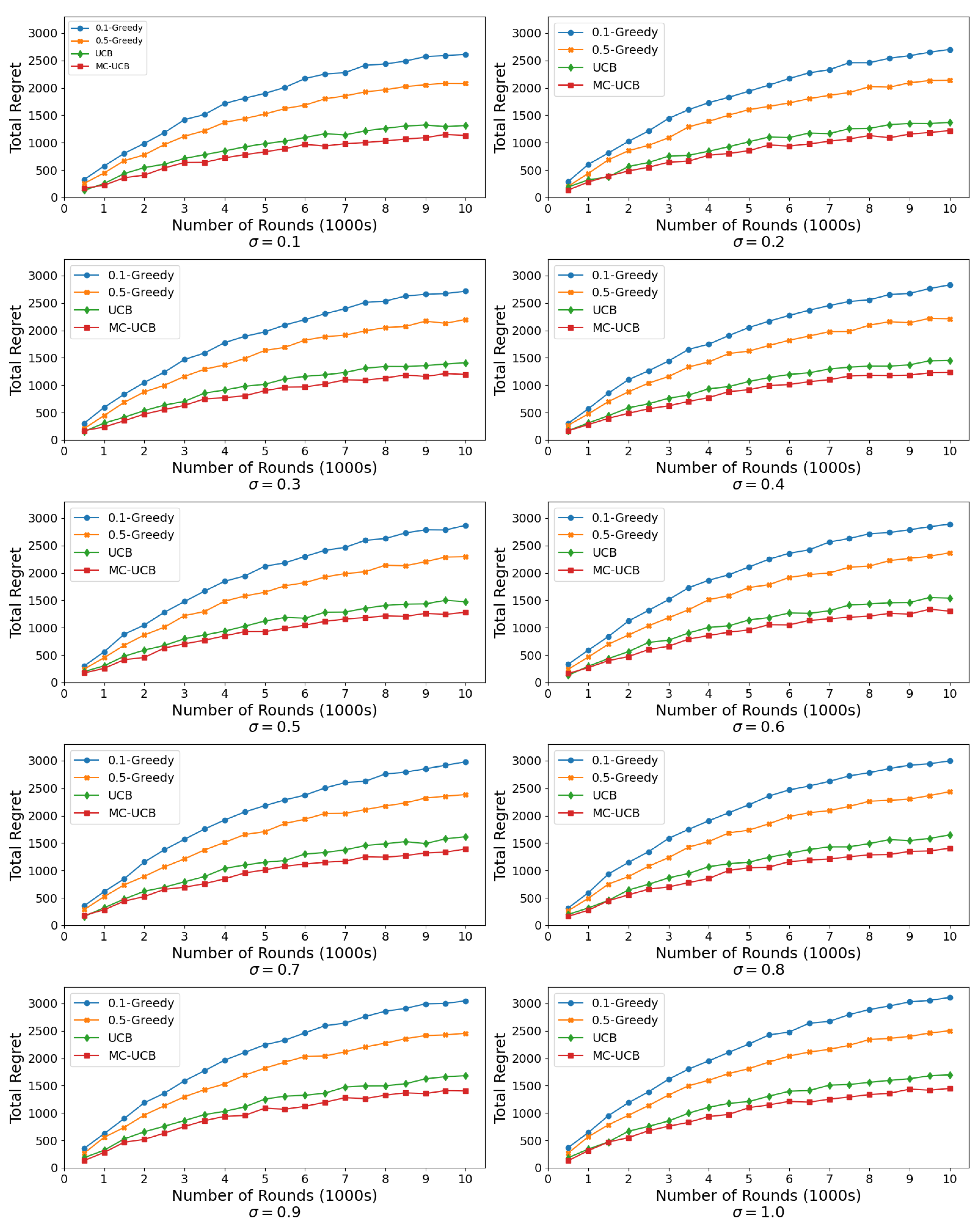
The results of the simulations are presented in Figure 2 and Figure 3, which illustrate the cumulative regret for the algorithms across multiple values of $\sigma$ (reward standard deviation) and the number of rounds. The comparison includes MC-UCB, UCB, and $ϵ$-Greedy with $ϵ=0.1$ and $ϵ=0.5$.

In Figure 2, we observe that as the value of $\sigma$ increases, the overall regret grows for all algorithms. However, the rate at which regret accumulates varies significantly across the algorithms. The MC-UCB algorithm consistently outperforms the baselines as it exhibits the lowest cumulative regret across all values of $\sigma$.

Specifically, the following trends can be identified:

• Effect of Increasing $\sigma$: As the value of $\sigma$ increases, the cumulative regret grows at a faster rate for all algorithms. This is expected because higher variability in rewards makes it more challenging to distinguish between the optimal and suboptimal arms. Nevertheless, MC-UCB demonstrates a robust ability to adapt to this increased variability and to maintain a clear performance advantage over the classical UCB and $ϵ$-Greedy algorithms.
• Comparison with $ϵ$-Greedy: The $ϵ$-Greedy algorithms, with $ϵ=0.1$ and $ϵ=0.5$, perform consistently worse than MC-UCB. Notably, $ϵ=0.5$ results in lower regret compared to $ϵ=0.1$, as the excessive exploration prevents the algorithm from exploiting the optimal arms efficiently. This is especially prominent in settings with low $\sigma$, where unnecessary exploration leads to regret accumulation.
• Performance of Classical UCB: The classical UCB algorithm achieves lower regret than the $ϵ$-Greedy variants but fails to match the performance of MC-UCB. The classical UCB assumes iid rewards and does not account for the Markovian structure, which limits its ability to leverage state transitions effectively. This leads to slower learning of the optimal arms.
• MC-UCB’s Adaptability: Across all settings of $\sigma$, MC-UCB demonstrates superior performance, particularly as the number of rounds increases. MC-UCB achieves faster convergence to the optimal arms and maintains lower cumulative regret by leveraging the Markovian structure. This advantage becomes more pronounced at higher $\sigma$ values, where the increased reward variability exacerbates the shortcomings of the baseline algorithms.

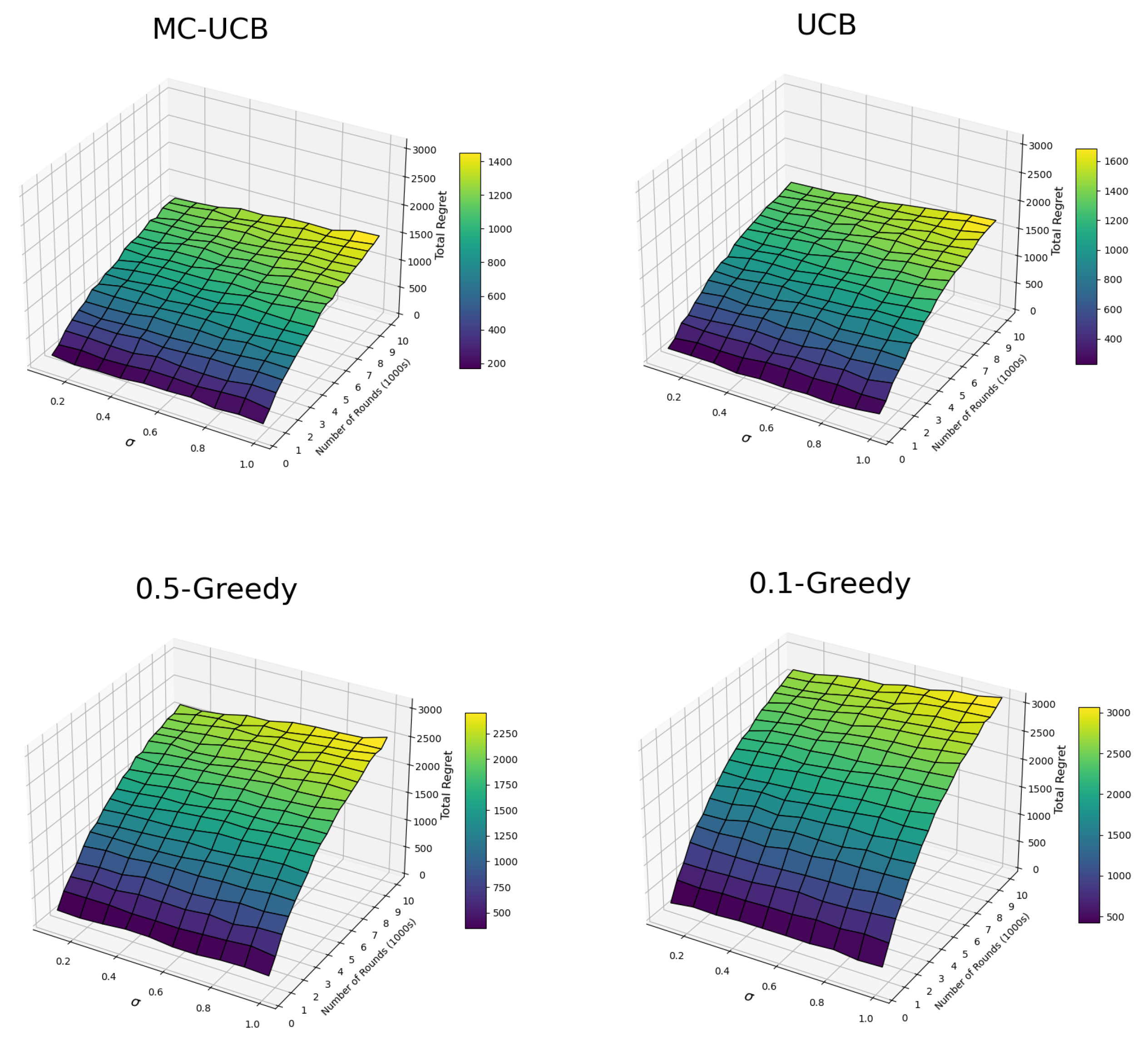
Figure 3 provides a three-dimensional view of the total regret for each algorithm as a function of $\sigma$ and the number of rounds. The plots reveal a clear trend: while all algorithms experience regret growth with increasing $\sigma$, MC-UCB consistently maintains the smallest regret surface. In contrast, the classical UCB and $ϵ$-Greedy algorithms exhibit higher regret surfaces, with $ϵ$-Greedy particularly struggling under larger $\sigma$ values.

6.4. Robustness and Sensitivity to System Variations

Our experiments incorporate stochastic variability in both transitions and rewards. While we have maintained fixed distributions for sampling these parameters, the repeated randomization and large number of runs ensure that the results are not tailored to a single contrived example. Over thousands of simulations, the MC-UCB algorithm consistently outperforms the baselines, indicating that its theoretical properties are robust to different random initializations and transitions. However, we must emphasize that these simulations remain limited in scale and scope. Larger state spaces could invalidate our current theoretical guarantees and cause the underlying assumptions of our derivations to fail.

6.5. Additional Markovian Network Scenario and Results

To further illustrate the flexibility of MC-UCB under a Markovian reward structure, we also conduct a complementary numerical experiment wherein the arms represent network links transitioning among three distinct quality states (High, Medium, and Low). The rewards are interpreted as throughput (in Mbps), reflecting the link’s capacity at each time step. Unlike the fully randomized approach in the previous settings, here we fix the transition matrices and reward means (sampled from the dataset [44]) to highlight how variability in observation noise (i.e., the standard deviation $\sigma$) impacts each algorithm’s performance.

We consider a simple network setting that translates to $K=3$ arms, each with a three-state Markov chain. The probability of remaining in or transitioning between these states is encoded by a fixed transition matrix $P^{\left(i\right)}$ for each arm $i\in \{1,2,3\}$. For example, an arm in a High state remains there with probability $0.80$, transitions to Medium with probability $0.15$, and drops to Low with probability $0.05$. We interpret the per-round reward $r_t^{\left(i\right)}$ as a throughput measurement drawn from a Gaussian distribution with mean ${\mu }_u^{\left(i\right)}$ (the average throughput for state u of arm i) and variance ${\sigma }^2$. Thus, higher reward corresponds to higher link throughput. We vary the standard deviation $\sigma \in \{2.0,3.0,4.0\}$ to simulate increasingly fluctuating network conditions.

We employ the same core policy classes introduced previously, with the key difference being that we now deal with throughput (Mbps) as reward:

• MC-UCB: Our proposed Markovian UCB policy that can exploit knowledge of the transition probabilities.
• Classical UCB: A reference baseline assuming iid rewards.
• Baseline-Greedy: A purely greedy strategy, always picking the arm with the highest observed average so far.

We set the horizon to T = 10,000 rounds. At each round, the selected arm yields a random throughput sample from $\mathcal{N}({\mu }_u^{\left(i\right)},{\sigma }^2)$ for its current state u, and all arms then transition. Our performance metric is the time-averaged throughput achieved by each policy, since throughput is a key measure of network performance.

For each fixed $\sigma$, we run three numerical evaluations on the network simulations (one for each policy) and compute the running average throughput over time. We then plot the final average–throughput curves for each policy. The transition matrices, state means, and values of $\sigma$ remain consistent in all runs to isolate the effect of observation noise (reward variability).

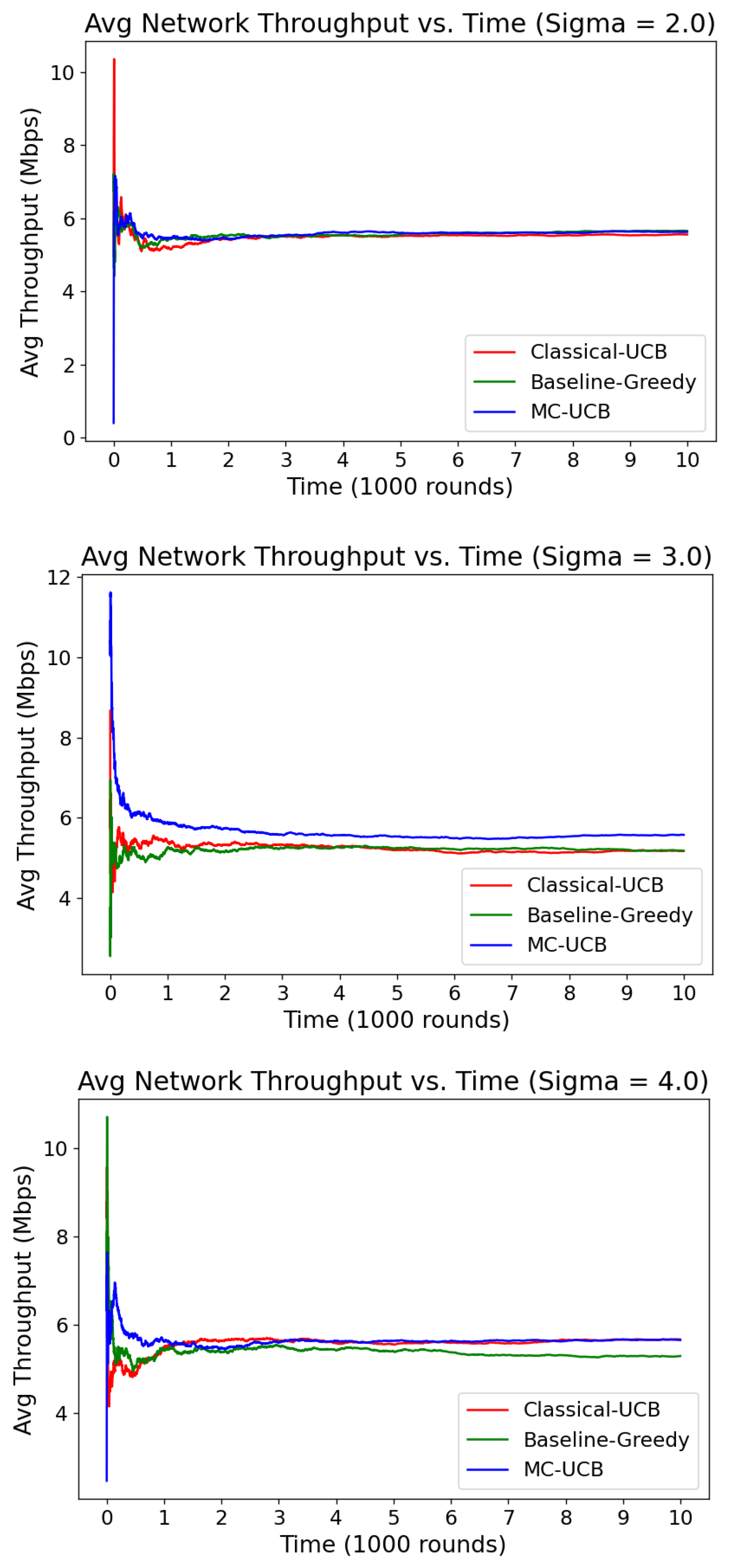
Figure 4 illustrates the key results for each $\sigma .$ The results clearly demonstrate the consistent superiority of the MC-UCB algorithm across all tested noise levels ($\sigma$). For $\sigma =2.0$, MC-UCB quickly stabilizes around 6 Mbps, outperforming both classical UCB and Baseline-Greedy, which exhibit slower convergence and slightly lower steady-state throughput. As the noise level increases to $\sigma =3.0$, MC-UCB maintains a noticeable advantage, achieving higher initial throughput and stabilizing at a value above 6 Mbps, whereas the other algorithms lag behind, converging closer to 5.5 Mbps. Even under the highest noise level, $\sigma =4.0$, MC-UCB continues to outperform its counterparts, demonstrating faster convergence and sustaining higher throughput near 6 Mbps, while classical UCB and Baseline-Greedy fall short. These results highlight the robustness and adaptability of MC-UCB, making it the most effective approach in scenarios with varying noise conditions.

6.6. Simulation Summary

Using purely synthetic data, the simulation results validate the effectiveness of the proposed MC-UCB algorithm within Markovian MAB settings, where it consistently surpasses classical UCB and $ϵ$-Greedy algorithms under various experimental conditions. Specifically, MC-UCB exhibits a $15\%$ lower cumulative regret on average compared to classical UCB for the specified settings. This demonstrates that MC-UCB successfully leverages the Markovian structure for efficient adaptation to state transitions. This is particularly evident as the reward variability increases (with a larger $\sigma$), where MC-UCB shows superior adaptability and maintains its performance advantage. This shows the robust adaptability of MC-UCB across scenarios with both low and high variability compared to the other baseline algorithms. The algorithm’s scalability is confirmed as MC-UCB’s regret curves ascend at a slower rate over increasing rounds, which showcases its long-term efficiency. The $ϵ$-Greedy algorithms, especially at $ϵ=0.1$, encounter issues with excessive exploitation in a way that leads to significantly higher regret. In contrast, while classical UCB performs better than $ϵ$-Greedy, it fails to match MC-UCB’s performance due to its inefficiency in handling state transitions. Overall, MC-UCB’s integration of the Markovian structure allows it to effectively balance exploration and exploitation.

Furthermore, in this supplemental experiment that we conducted on the simulated network and that was derived from the dataset in [44], the Markovian perspective allows our MC-UCB algorithm to handle state transitions adeptly, which translates to more stable performance in highly variable settings (large $\sigma$) and to higher throughput overall. This supplemental experiment thus complements the more extensive randomized evaluations by focusing on a single, fixed set of state transitions under network settings, which further highlights MC-UCB’s efficacy in network-like applications.

7. Conclusions

In this study, we have addressed the multi-armed bandit (MAB) problem with a Markovian rewards structure where each arm can transition between up to three states, which simulates dependencies often seen in networked systems. We demonstrated that a sample mean-based index policy, when adjusted for the complexity of our model, achieves logarithmic regret uniformly over time. This effectiveness depends on setting the exploration constant large enough relative to the eigenvalue gaps of the arms’ stochastic matrices. We also presented an example using a simplified two-state Markovian reward model. The numerical analysis suggests that the index policy remains near optimal even if the exploration constant does not strictly meet the theoretical sufficiency condition. This robustness indicates that our policy can be effective in a wide range of practical scenarios, including applications with network-like dependencies.