A Computationally Efficient Gradient Algorithm for Downlink Training Sequence Optimization in FDD Massive MIMO Systems

Abstract

Future wireless networks will require advance physical-layer techniques to meet the requirements of Internet of Everything (IoE) applications and massive communication systems. To this end, a massive MIMO (m-MIMO) system is to date considered one of the key technologies for future wireless networks. This is due to the capability of m-MIMO to bring a significant improvement in the spectral efficiency and energy efficiency. However, designing an efficient downlink (DL) training sequence for fast channel state information (CSI) estimation, i.e., with limited coherence time, in a frequency division duplex (FDD) m-MIMO system when users exhibit different correlation patterns, i.e., span distinct channel covariance matrices, is to date very challenging. Although advanced iterative algorithms have been developed to address this challenge, they exhibit slow convergence speed and thus deliver high latency and computational complexity. To overcome this challenge, we propose a computationally efficient conjugate gradient-descent (CGD) algorithm based on the Riemannian manifold in order to optimize the DL training sequence at base station (BS), while improving the convergence rate to provide a fast CSI estimation for an FDD m-MIMO system. To this end, the sum rate and the computational complexity performances of the proposed training solution are compared with the state-of-the-art iterative algorithms. The results show that the proposed training solution maximizes the achievable sum rate performance, while delivering a lower overall computational complexity owing to a faster convergence rate in comparison to the state-of-the-art iterative algorithms.

1. Introduction

The rapid growth in the number of smart devices and the emergence of the Internet of Everything (IoE) applications, which require an ultra-reliable and low-latency communication, will result in a substantial burden on the current wireless networks [1]. As such, the data rate that could be supplied by current wireless networks will be unlikely to sustain the enormous ongoing data traffic explosion. In addition, the latest statistics revealed that by 2023 nearly two-thirds of the global population will have Internet access with around 5.3 billion Internet users (66 percent of the global population), and by 2025 more than 80 billion devices will require communication connectivity [2]. Therefore, this will create the requirements for massive communication systems and networks. These requirements and demands for data traffic have motivated research into continuing to advance the existing networks in addition to the innovation of new physical-layer techniques for the future generation of cellular systems. Massive MIMO (m-MIMO) is introduced as a key physical layer technique for the next generation wireless networks that is required to support the huge increasing demand for data traffic [3,4,5], whilst improving the energy efficiency [6]. In particular, the m-MIMO system is considered a potential solution for fifth generation (5G) wireless communications and beyond [7]. However, from an information theoretic point of view, the performance of the m-MIMO system depends on the accuracy and availability of the channel state information (CSI) estimation. Obtaining the CSI at the BS depends on the duplexing operation mode, i.e., either frequency division duplex (FDD) or time division duplex (TDD) mode. Despite the promising results of TDD operation with m-MIMO when it comes to the CSI estimation, the vast majority of the currently deployed cellular networks operates in FDD mode. For example, over 85% of the current commercial long term evolution (LTE) wireless mobile networks operate in FDD mode [8]. Therefore, this paper focuses on FDD systems, as the CSI can only be obtained by a dedicated training sequence in the downlink (DL). In particular, to obtain the CSI in FDD systems, the BS needs to optimize the DL training sequence and transmit it to the users [9,10]. However, the expansion of a number of antenna elements at the BS in the m-MIMO system makes the DL training sequence optimization for fast CSI estimation, i.e., with limited coherence time, in FDD systems very challenging.

To overcome the CSI estimation challenge in FDD m-MIMO systems, several studies have investigated the optimization of DL training sequences by considering the scenario where the users exhibit common spatial correlation at the BS under different system model assumptions; namely, refs. [11,12,13,14,15,16,17,18] exploit correlations in the spatial domain and correlations both in the time and spatial domains, respectively. However, in practice, users could exhibit distinct spatial correlation patterns, which arise due to independent propagation conditions and scattering geometries; hence, the optimization framework of the training sequences developed in [11,12,13,14,15,16,17,18] does not hold in general multiuser scenarios with K distinct spatial correlations. Another line of research has focused on the channel estimation by using compressed sensing (CS) based techniques [19,20,21,22,23,24]. However, due to the unknown sparse nature of the channels, CS based approaches cannot be applied in practice to predict the DL achievable sum rate of an FDD m-MIMO system. Another development for CSI estimation is to use a hybrid two-stage precoding approaches, see e.g.,  [25,26,27,28]. However, the aforementioned research works do not address the single-stage precoding scenario with K independent user covariance matrices.

To address the challenge of having distinct correlated channels and to find a more realistic solution with single-stage precoding scheme, several studies have investigated the design of training sequences by utilizing different iterative algorithms. For example, in [29] the DL training sequences are optimized iteratively based on the average sum rate loss due to CSI estimation with zero forcing (ZF) precoding. In refs. [30,31] the DL training sequences are optimized iteratively as a solution to a sum conditional mutual information (SCMI) maximization problem and a sum mean square error (SMSE) minimization problem, respectively. While the investigations in refs. [30,31] have optimized the DL training sequences iteratively, the algorithms used in the optimization exhibit slow convergence speed, and thus, deliver high latency and computational complexity. However, in real-time systems, the CSI estimation must be obtained more frequently with an acceptable latency from channel estimation to precoding, especially when the channel exhibits a shorter coherence time. Therefore, there is an essential requirement for developing a new efficient iterative algorithm for the FDD m-MIMO systems that optimizes the DL training sequence, i.e., maximizes the sum rate, while at the same time exhibits the fast convergence rate so as to obtain the CSI estimation more quickly over a limited coherence time. Note that the design principles in refs. [30,31] are more general compared with [29] since they do not enforce a specific precoding structure and do not consider a heuristic approximate upper bound of the sum rate loss for CSI estimation. This makes the approaches in refs. [30,31] more rigorous than the approach in [29] for DL sequences optimization.

This paper addresses the challenge of CSI DL channel estimation in the FDD m-MIMO systems with limited coherence time considering the users have different correlations. We propose a conjugate gradient descent (CGD) optimization algorithm over the Riemannian manifold for optimizing the DL training sequences. The proposed algorithm is essentially required to speed up the convergence rate by lessening the required number of iterations for achieving fast CSI estimation and hence reduces the overall computational complexity. This proposed algorithm is also very useful for massive communication systems and networks. In this paper, a random matrix theory (RMT) method [32,33] is used to validate our Monte-Carlo simulations. This allows the achievement of a straightforward methodology without resorting to a computationally demanding exhaustive search. In addition, the computational complexity analyses of the proposed CGD algorithm and the state-of-the-art SCMI [30] and SMSE [31] iterative algorithms are provided. 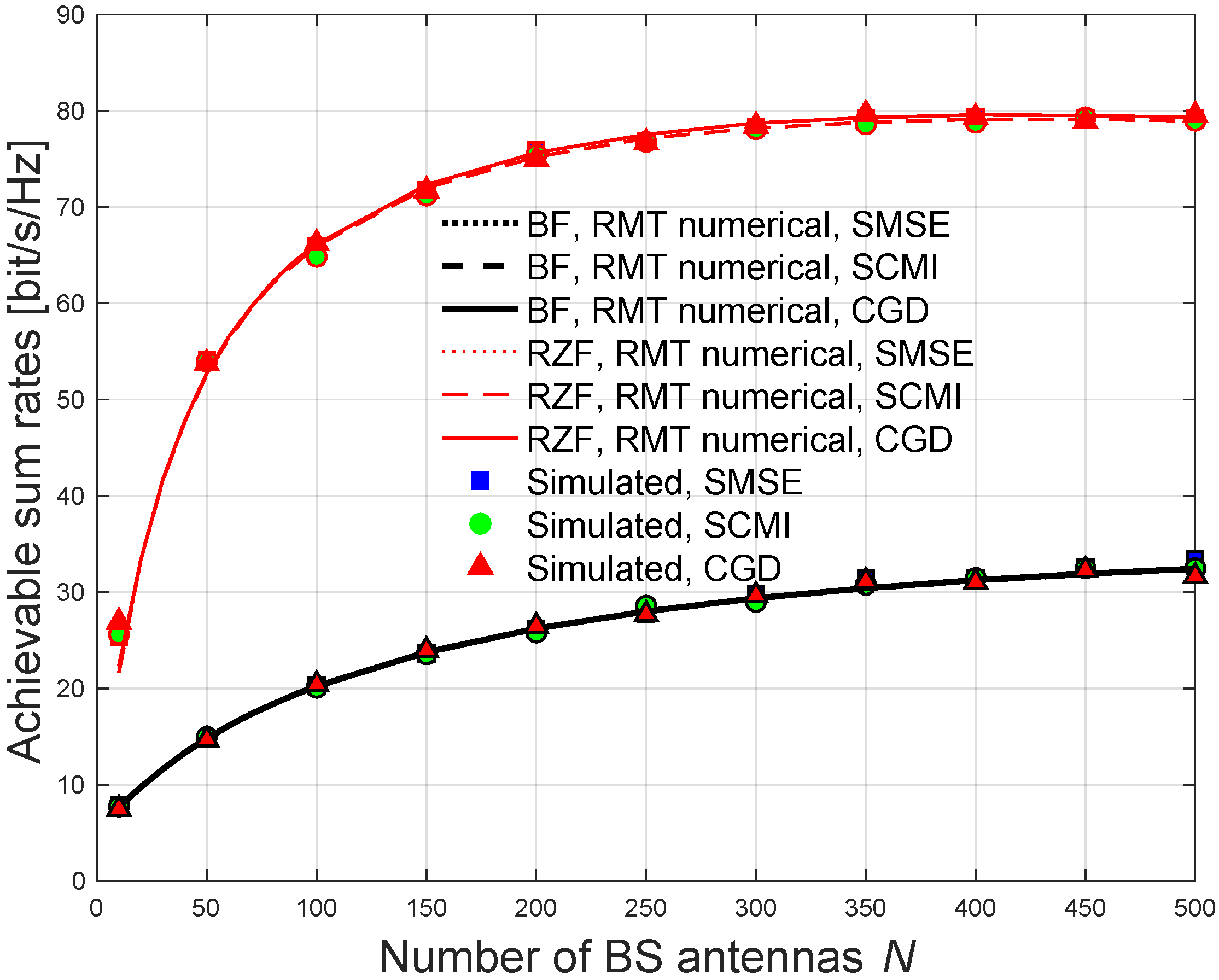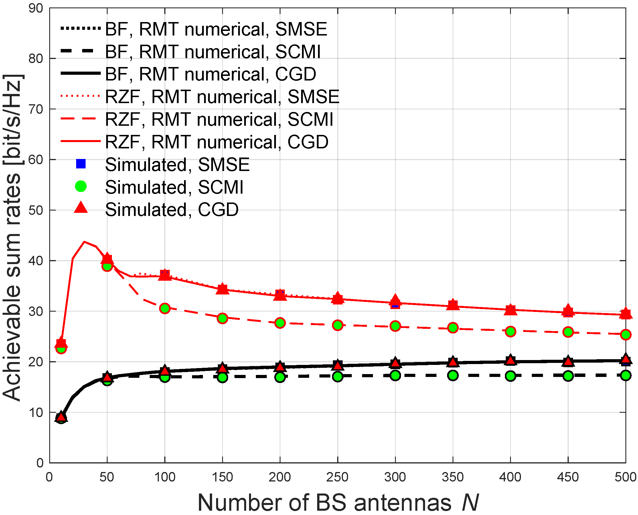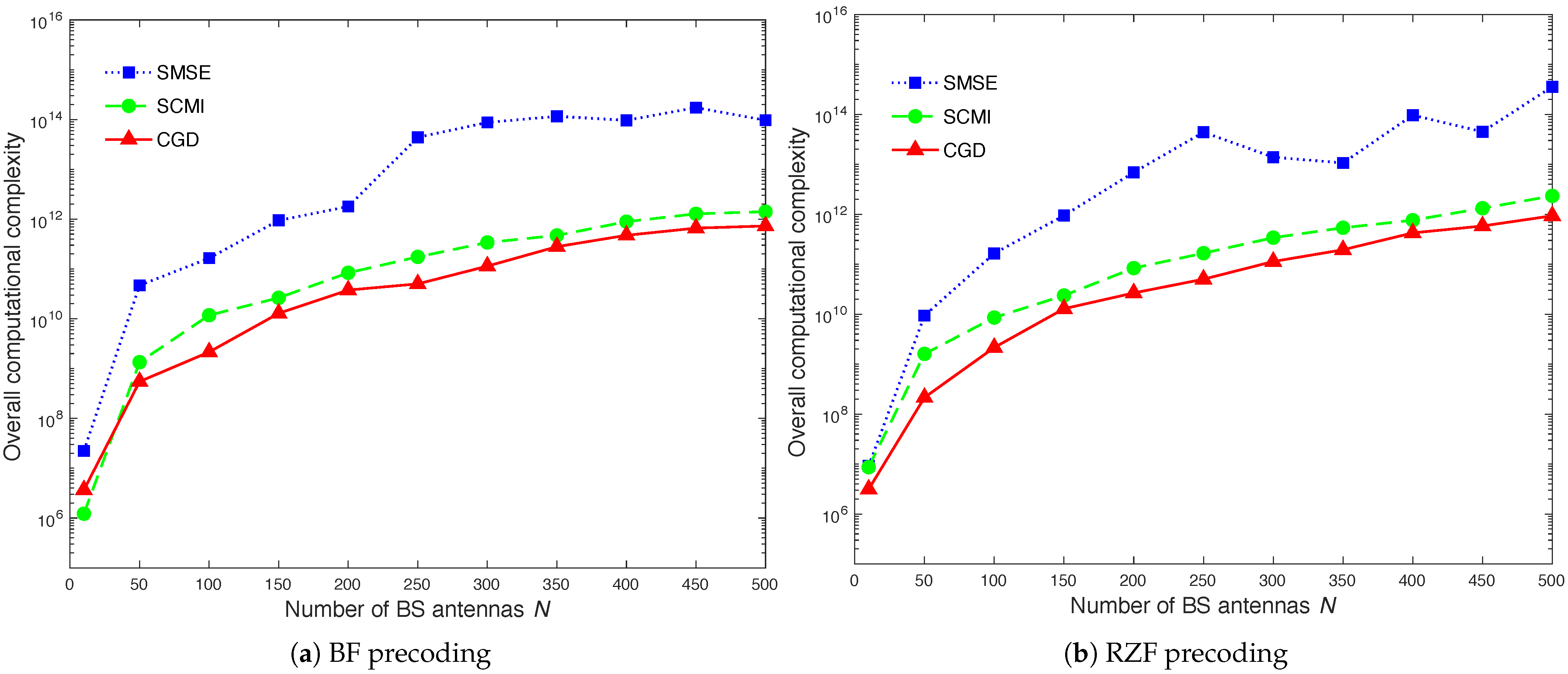Comparisons are presented for the sum rate and overall complexity performances between the proposed CGD algorithm and existing SCMI [30] and SMSE [31] iterative algorithms for DL sequence optimization in both eigenbeamforming (BF) and the regularized ZF (RZF) precoding. The aforementioned algorithms are considered the best known state-of-the-art iterative algorithms. The results demonstrate that the RZF precoder under correlated channels achieves a significant gain in the DL sum rate in comparison to the BF precoder. The results show that the proposed CGD algorithm achieves more or less the same rate performances as the state-of-the-art iterative algorithms for training designs, while reducing the computational complexity in both BF and RZF precoding. This computational complexity reduction is due to the use of matrix exponential search over the Riemannian manifold, which results in an optimized DL training sequence for fast CSI estimation in the FDD m-MIMO systems. These findings create a pathway for realizing FDD m-MIMO with massive communication systems. Finally, the results demonstrate that the analytical solution using the RMT method tightly agrees with the simulation, which underpins the contributions of this paper.

The present paper is organized as follows: in Section 2, the system model is described. In Section 3, the training sequence design in an FDD m-MIMO system is investigated. In Section 4, the CGD iterative algorithm is developed. In Section 5, the expressions that accurately approximate the SINR and the DL achievable sum rate are introduced. In Section 6, the results are presented and discussed. Finally, in Section 7, the conclusions are drawn.

Notation: In this paper, an upper boldface symbol denotes a matrix whereas a lower boldface symbol denotes a vector. The term $\mathbb{E}[·]$ refers to the expectation operator. The operators trace, transpose, Hermitian transpose, inverse and absolute value are denoted by $\mathrm{tr}(·)$, ${(·)}^{\mathrm{T}}$, ${(·)}^{\mathrm{H}}$, ${(·)}^{-1}$, and $|·|$, respectively.

2. System Model Description

This paper considers a single-cell wireless communications system, where the BS is equipped with an N transmit antenna that serves K single antenna users. We consider a non-line-of-sight (NLOS) Rayleigh fading channels over a single-frequency band with an overall coherence time denoted by $T_{}\in {\mathbb{Z}}^{+}$ and enumerated in symbols per transmission block. Figure 1 demonstrates a BS with m-MIMO system and illustrates the DL and UL transmissions within each coherence block length. The  received signal during the data transmission phase at the k-th user is given as:

$$\begin{array}{c}\hfill y_k^{}=\sqrt{{\rho }_{\mathrm{d}}^{}\lambda }{\mathbf{h}}_k^{\mathrm{H}}\mathbf{V}\mathbf{s}+z_k^{}\end{array}$$

(1)

where ${\rho }_{\mathrm{d}}$ denotes the per-user signal-to-noise-ratio (SNR) during the data transmission phase and $\lambda$ refers to the normalization constant, which is defined as $\lambda =K/\mathbb{E}\left[\mathrm{tr}\left({\mathbf{VV}}^{\mathrm{H}}\right)\right]$, and $\mathbf{V}=[{\mathbf{v}}_1,\dots ,{\mathbf{v}}_K]\in {\mathbb{C}}^{N\times K}$ is the precoding matrix. The term $\mathbf{s}={[s_1,\dots ,s_K]}^{\mathrm{T}}\in {\mathbb{C}}^K$ is independently and identically distributed (IID) with a zero mean circularly symmetric complex Gaussian (CSCG) vector of data symbols, which satisfies $\mathbb{E}\left[\mathbf{s}{\mathbf{s}}^{\mathrm{H}}\right]={\mathbf{I}}_K$, and $z_k$ denotes the additive noise, which is modeled as a zero mean unit variance CSCG random variable. The DL instantaneous channel vector is given by ${\mathbf{h}}_k={\mathbf{R}}_k^{1/2}{\tilde{\mathbf{h}}}_k^{}$, where the elements of ${\tilde{\mathbf{h}}}_k\in {\mathbb{C}}^N$ are IID with zero mean and unit variance and k-th user’s correlation matrix, ${\mathbf{R}}_k$ satisfies ${\mathbf{R}}_k=\mathbb{E}\left[{\mathbf{h}}_k^{}{\mathbf{h}}_k^{\mathrm{H}}\right]\in {\mathbb{C}}^{N\times N}$. It is worth noting that ${\mathbf{R}}_k$ depends on large-scale statistics, i.e., angles of arrival and departure or spatial/temporal correlation, which are considered to be frequency-invariant, and thus, can be efficiently obtained in the FDD or TDD systems [34]. To this end, the received signal-to-interference-plus-noise ratio ($\mathrm{SINR}$), denoted ${\gamma }_k$, is given as:

$${\gamma }_k=\frac{\lambda \mid \mathbb{E}\left[{\mathbf{h}}_k^{\mathrm{H}}{\mathbf{v}}_k^{}\right]{\mid }^2}{\frac{1}{{\rho }_{\mathrm{d}}^{}}+\lambda \mathbb{E}\left[|{\mathbf{h}}_k^{\mathrm{H}}{\mathbf{v}}_k^{}-\mathbb{E}\left[{\mathbf{h}}_k^{\mathrm{H}}{\mathbf{v}}_k^{}\right]{|}^2\right]+\lambda {\sum }_{l\ne k}^K\mathbb{E}\left[|{\mathbf{h}}_k^{\mathrm{H}}{\mathbf{v}}_l^{}{|}^2\right]}$$

(2)

Accordingly, the DL achievable sum rate, $C_{}^{}$, for an FDD m-MIMO system under consideration can be expressed as:

$$C_{}^{}=\left(1-\frac{T_{\mathrm{tr}}^{}}{T_{}^{}}\right)\sum _{k=1}^K{\log }_2^{}\left(1+{\gamma }_k^{}\right)[\mathrm{bit}/\mathrm{s}/\mathrm{Hz}]$$

(3)

where parameter $T_{\mathrm{tr}}$ represents the training sequence length used during the training-phase. This paper uses $T_{\mathrm{tr}}$ that maximizes the achievable sum rate. The received SINR term in (2) depends on the channel statistics, the channel estimates, and the linear precoding technique used at the BS. We consider two commonly prevailing types of linear precoders, named the BF and the RZF, as defined in [33]. The expectation (i.e., the averaging process) in (2) is taken with respect to different channel realizations, which are obtained separately by means of Monte Carlo simulation. As the purpose of the present paper is to concentrate on the DL training sequence design, the UL feedback time and associated error rate are assumed to be zero. Efficient feedback schemes can be considered in the future, see, e.g., [35,36,37,38]. Besides, advanced signal processing techniques can also be considered for feedback, see e.g., [39,40]. A large system limit based on random matrix theory methods is used to provide asymptotic expressions that accurately approximate the SINR and achievable sum rate for the BF and RZF precoders.

3. CSI Estimation Using DL Training Sequences

To gain further insight into the problem of DL CSI estimation, this section investigates the training sequence design in an FDD m-MIMO system. To estimate the DL channel, the BS transmits a predetermined training sequence of length $T_{\mathrm{tr}}$ during the training-phase. The DL pilot sequences, collected by each user and returned to the BS, provide instantaneous channel realizations at the BS, which in turn implement regular BF or RZF precoding based on channel estimates. As such, the training sequences for channel estimation [41] are updated according to the dynamics of each ${\mathbf{R}}_k$, which in turn is updated at every coherence time interval. To this end, the received signal during training-phase, ${\mathbf{y}}_k^{}\in {\mathbb{C}}^{T_{\mathrm{tr}}}$, at the k-th user is given by:

$${\mathbf{y}}_k^{}=\sqrt{{\rho }_{\mathrm{tr}}^{}}{\mathbf{S}}_{\mathrm{tr}}^{\mathrm{H}}{\mathbf{h}}_k^{}+{\mathbf{z}}_k^{}$$

(4)

where ${\mathbf{S}}_{\mathrm{tr}}^{}\in {\mathbb{C}}^{N\times T_{\mathrm{tr}}^{}}$ is the training matrix. The receiver noise ${\mathbf{z}}_k\in {\mathbb{C}}^{T_{\mathrm{tr}}}$ exhibits a CSCG distribution $\mathcal{CN}\left(\mathbf{0},{\mathbf{I}}_{T_{\mathrm{tr}}}\right)$.

Extensive research has been carried out to address the challenge of CSI estimation, see e.g., [11,12,13,14,15,16,17,18]. In these investigations, a special scenario when the users exhibit common spatial correlation at the BS is considered. However, a more general scenario when the users exhibit distinct spatial correlation at the BS is needed. Besides, compressed sensing based approaches for CSI estimation have been used in [19,20,21,22,23,24]. In these works, the sparsity structure on the virtual angular domain is used to reduce the training length required for the CSI estimation. However, the compressed sensing based approaches cannot be applied in practice due to the unknown sparsity nature of the channels that cannot be predicted in these approaches. Another area of research on CSI estimation is to exploit the hybrid two-stage precoding based approaches, see e.g.,  [25,26,27,28]. In particular, the hybrid based approaches exploit correlation in the spatial domain, where the users within each group exhibit the same spatial correlation, and a linear superposition of each group correlation matrix is utilized to perform the first of two stages of precoding, thus forming a beam for each group. However, sophisticated scheduling and clustering algorithms of the user groups, and of the users inside each group, are required in these hybrid approaches. Hence, these works cannot be applied to predict the achievable sum rate performance in a more general single-stage scenario with K independent user covariance matrices. To address the challenge of CSI estimation in the more general single-stage precoding scenario when the users exhibit distinct correlated channels, several studies have been carried out, see, e.g.,  [30,31,42,43]. Specifically, the training sequences in [30,31,42,43] are designed by exploiting different iterative algorithms as a solution to an SCMI maximization criterion and an SMSE minimization criterion, respectively. However, the limited coherence time interval in practice implies that the CSI estimation should be determined more frequently, and thus, iterative-based solutions for the DL training sequence design may be infeasible. In addition, the algorithms used in the aforementioned optimizations exhibit slow convergence speed, and thus, deliver high latency and computational complexity. Hence, there is a crucial need to develop a lower complexity iterative algorithm solution for the FDD m-MIMO systems, which has the ability to optimize the DL training sequence, i.e., maximizes the achievable sum rate, while at the same time exhibits a fast convergence rate so that obtaining a fast CSI estimation when a limited coherence time is considered.

This paper proposes a computationally efficient CGD iterative algorithm, described in detail in Section 4, to optimize ${\mathbf{S}}_{\mathrm{tr}}$ for pre-selected training length $T_{\mathrm{tr}}$, and training power ${\rho }_{\mathrm{tr}}^{}$. The proposed algorithm aims to achieve a robust sum rate performance when the users exhibit different correlations while at the same time reducing the computational complexity. Let $f\left({\mathbf{S}}_{\mathrm{tr}}\right)\in \mathbb{R}$ denote the sum MSE of the channel estimate cost function, which needs to be minimized with respect to the DL training matrix ${\mathbf{S}}_{\mathrm{tr}}$, as 

$$f\left({\mathbf{S}}_{\mathrm{tr}}\right)=\sum _{k=1}^K\mathrm{tr}\left({\mathbf{R}}_k\right)-\sum _{k=1}^K\mathrm{tr}\left({\mathsf{\Phi }}_k\right)$$

(5)

where ${\mathsf{\Phi }}_k={\mathbf{R}}_k^{}{\mathbf{S}}_{\mathrm{tr}}^{}{\left({\mathbf{S}}_{\mathrm{tr}}^{\mathrm{H}}{\mathbf{R}}_k^{}{\mathbf{S}}_{\mathrm{tr}}^{}+\frac{1}{{\rho }_{\mathrm{tr}}^{}}{\mathbf{I}}_{T_{\mathrm{tr}}^{}}^{}\right)}^{-1}{\mathbf{S}}_{\mathrm{tr}}^{\mathrm{H}}{\mathbf{R}}_k^{}$, which denotes the k-th user’s covariance matrix with minimum mean square error (MMSE) channel estimation. To this end, the formulation of the CSI estimation optimization problem is provided. Minimizing the sum MSE over the training sequence ${\mathbf{S}}_{\mathrm{tr}}^{}$ for a given training-phase duration $T_{\mathrm{tr}}$ in the FDD m-MIMO system equates to the optimization problem defined in (6).

$$\begin{array}{cc}\hfill & \underset{{\mathbf{S}}_{\mathrm{tr}}}{\mathrm{minimize}}f\left({\mathbf{S}}_{\mathrm{tr}}\right)\hfill \\ \hfill & \mathrm{subject}\mathrm{to}{\mathbf{S}}_{\mathrm{tr}}^{\mathrm{H}}{\mathbf{S}}_{\mathrm{tr}}^{}={\mathbf{I}}_{T_{\mathrm{tr}}}\hfill \end{array}$$

(6)

The sum MSE cost function, which corresponds to a function of the subspace that is spanned by the pilot matrix ${\mathbf{S}}_{\mathrm{tr}}$, is invariant to the unitary rotation, i.e., $f\left({\mathbf{S}}_{\mathrm{tr}}\mathbf{U}\right)=f\left({\mathbf{S}}_{\mathrm{tr}}\right)$.

This property allows the CGD algorithm over the Riemannian manifold to be effectively used to solve the optimization problem in (6). To apply the CGD optimization algorithm on a Riemannian manifold, the partial derivative of the sum MSE cost function in (5) needs to be determined with respect to ${\mathbf{S}}_{\mathrm{tr}}$. To this end, the partial derivative $\mathsf{\Gamma }\in {\mathbb{C}}^{N\times T_{\mathrm{tr}}}$ is given by [31]:    

$$\begin{array}{c}\hfill \mathsf{\Gamma }=2\sum _{k=1}^K(-{\mathbf{R}}_k^2{\mathbf{S}}_{\mathrm{tr}}^{}{\left({\mathbf{S}}_{\mathrm{tr}}^{\mathrm{H}}{\mathbf{R}}_k^{}{\mathbf{S}}_{\mathrm{tr}}^{}+\frac{1}{{\rho }_{\mathrm{tr}}^{}}{\mathbf{I}}_{T_{\mathrm{tr}}^{}}^{}\right)}^{-1}+{\mathbf{R}}_k^{}{\mathbf{S}}_{\mathrm{tr}}^{}\times \\ \hfill {\left({\mathbf{S}}_{\mathrm{tr}}^{\mathrm{H}}{\mathbf{R}}_k^{}{\mathbf{S}}_{\mathrm{tr}}^{}+\frac{1}{{\rho }_{\mathrm{tr}}^{}}{\mathbf{I}}_{T_{\mathrm{tr}}^{}}^{}\right)}^{-1}{\mathbf{S}}_{\mathrm{tr}}^{\mathrm{H}}{\mathbf{R}}_k^2{\mathbf{S}}_{\mathrm{tr}}^{}{\left({\mathbf{S}}_{\mathrm{tr}}^{\mathrm{H}}{\mathbf{R}}_k^{}{\mathbf{S}}_{\mathrm{tr}}^{}+\frac{1}{{\rho }_{\mathrm{tr}}^{}}{\mathbf{I}}_{T_{\mathrm{tr}}^{}}^{}\right)}^{-1})\end{array}$$

(7)

where the right hand side in (7) is obtained by differentiating the cost function in (6) with respect to pilot matrix, (i.e., $\partial f\left({\mathbf{S}}_{\mathrm{tr}}\right)/\partial {\mathbf{S}}_{\mathrm{tr}}^{*}$).

4. Training Sequence Optimization Based on CGD Algorithm over the Riemannian Manifold

Optimization on manifolds means finding an optimum solution of a desired function using a smooth finite-dimensional Riemannian manifold. The Riemannian gradient is simply the orthogonal projection of the classical gradient. Conceptually, the key point is to perform as unconstrained nonlinear optimization. Exploiting the Riemannian makes it easy to deal with various types of constraints, which arise in low rank matrices. In particular, optimization on manifolds is a powerful scheme to address the nonlinear optimization problems such as the problem of finding the training sequence matrix that maximizes the achievable sum rate of the FDD massive MIMO systems, which is considered in this present paper. In wireless communication systems and array signal processing, several studies have considered various optimization problems under a unitary matrix constraint [44,45,46,47]. Consequently, advanced gradient-based iterative algorithms have been developed to find efficient solutions with fast convergence rate to such optimization problems [48,49,50,51]. Some of those efficient solutions have been obtained using a geometrical approach based on the smooth parameter space known as the Riemannian manifold. The potential of the Riemannian manifold has motivated the author of this paper to explore the application of such a geometrical approach for optimising the training sequence in an FDD massive MIMO system when the users exhibit distinct spatial correlations. In this section, the CGD iterative algorithm based on the Riemannian manifold is explored to optimize the DL pilot matrix ${\mathbf{S}}_{\mathrm{tr}}$ iteratively across multiple users with independent channel covariance matrices. In optimizing (6) for ${\mathbf{S}}_{\mathrm{tr}}$, the CGD method uses the almost periodic property of the matrix exponential search [52,53] over the Riemannian manifold to increase the algorithm convergence speed by lessening the required number of iterations. In particular, the introduction of matrix exponential on the Riemannian manifold aids the proposed CGD algorithm to operate over a smaller dimensional search space and thus provide a fast convergence behaviour. In addition, the existence of matrix exponential parametrization in the proposed CGD method is a sufficient condition to satisfy the semi-unitary matrices ${\mathbf{S}}_{\mathrm{tr}}^{\mathrm{H}}{\mathbf{S}}_{\mathrm{tr}}^{}={\mathbf{I}}_{T_{\mathrm{tr}}}$. Further details on the matrix exponential property on the Riemannian manifold can be found in [52,53,54]. This algorithm can also be used to increase the capacity with interference channel [55]. Algorithm 1 summarizes the proposed CGD iterative algorithm. The following steps explain Algorithm 1 in further detail.

Algorithm 1 Iterative CGD optimization algorithm.

1: $\mathrm{Initialization}:t=0\mathrm{and}\mu =1, {\mathbf{S}}_t={\mathbf{I}}_{}\in {\mathbb{C}}^{N\times T_{\mathrm{tr}}}$ 2: Determine the gradient using (8), and set ${\mathbf{G}}_t={\mathbf{D}}_t.$ 3: $\mathrm{If}\langle {\mathbf{D}}_t,{\mathbf{D}}_t\rangle <ϵ,\mathrm{then}\mathrm{break}.$ 4: $\mathrm{Determine}\mathrm{the}\mathrm{matrix}\mathrm{exponential}:{\mathbf{P}}_t=\exp (-\mu {\mathbf{D}}_t).$ 5: $\mathrm{If}f\left({\mathbf{S}}_t\right)-f\left({\mathbf{P}}_t{\mathbf{S}}_t\right)\ge \mu \langle {\mathbf{D}}_t,{\mathbf{D}}_t\rangle ,\mathrm{double}{\mathbf{P}}_t,\mu :=2\mu .$ 6: $\mathrm{If}f\left({\mathbf{S}}_t\right)-f\left({\mathbf{P}}_t{\mathbf{S}}_t\right)<0.5\mu \langle {\mathbf{D}}_t,{\mathbf{D}}_t\rangle ,\mathrm{halve}{\mathbf{P}}_t,\mu :=0.5\mu .$ 7: $\mathrm{Update}{\mathbf{S}}_{t+1}:={\mathbf{P}}_t{\mathbf{S}}_t$. 8: $\mathrm{Update}{\mathbf{G}}_{t+1}={\mathbf{D}}_{t+1}+{\upsilon }_t{\mathbf{G}}_t,t:=t+1,\mathrm{and}\mathrm{go}\mathrm{to}\mathrm{step}2$.

• Step 1—Initial step: The proposed iterative gradient algorithm starts by selecting an initial training sequence matrix ${\mathbf{S}}_{\mathrm{tr}}\in {\mathbb{C}}^{N\times T_{\mathrm{tr}}}$. For the sake of notational simplicity, in the algorithm, the training sequence matrix notation ${\mathbf{S}}_{\mathrm{t}}$ is used instead, where the subscript t corresponds to the number of iterations.
• Step 2—Gradient evaluation and projection on the Riemannian parameter space: In this step, the gradient of the sum MSE cost function defined in (5) is determined, and the projection on the Riemannian manifold is computed to find the descent direction and set ${\mathbf{G}}_t={\mathbf{D}}_t$.

  $${\mathbf{D}}_t={\mathsf{\Gamma }}_t^{}{\mathbf{S}}_t^{\mathrm{H}}-{\mathbf{S}}_t^{}{\mathsf{\Gamma }}_t^{\mathrm{H}}$$

  (8)

  where ${\mathbf{D}}_t$ is the descent direction for iteration t and ${\mathsf{\Gamma }}_t$ corresponds to the Euclidean gradient with respect to the training sequence matrix as given in (7).
• Step 3—Stopping criteria: Check the gradient on the Riemannian parameter space (i.e., ${\mathbf{D}}_t$) whether it reaches convergence or not according to:

  $$\langle {\mathbf{D}}_t,{\mathbf{D}}_t\rangle =\frac{1}{2}\mathrm{Re}\left\{\mathrm{tr}\left({\mathbf{D}}_t^{\mathrm{H}}{\mathbf{D}}_t^{}\right)\right\}$$

  (9)

  where Re stands for the real value and $ϵ$ in step 3 of Algorithm 1 denotes the error tolerance. If the steepest direction is sufficiently small, which implies a close to local minimum value of the cost function the algorithm stops.
• Step 4—Matrix exponential computation: Determine the local parametrisation based on the matrix exponential on the Riemannian manifold, i.e., ${\mathbf{P}}_t=\exp (-\mu {\mathbf{D}}_t)$, where $\mu$ corresponds to the step size that controls the steepest direction. The complex matrix exponential is determined by the convergent power series [52,53], where a Matlab function expm is used for this purpose.
• Steps 5 and 6—Step size evaluation: The step size $\mu$ is required to be tuned in order to ensure an appropriate steepest direction movement towards the training solution. In particular, in steps 5 and 6, the sum MSE cost function of different sequences are evaluated based on different possibilities of $\mu$. If $\mu$ is too small and the condition of the cost function is not met, then $\mu$ is doubled, as given in step 5. If $\mu$ is too large and the condition of the cost function is not met, then $\mu$ is halved, as provided in step 6.
• Step 7—Updating the training sequence and the gradient direction: In this step, the pilot matrix and the gradient direction are updated according to the obtained matrix exponential ${\mathbf{P}}_t$. Due to the unitary invariant rotation of the cost function, the obtained training sequence has unitary columns.
• Step 8—The new conjugate gradient direction is obtained by updating ${\mathbf{G}}_{t+1}={\mathbf{D}}_{t+1}+{\upsilon }_t{\mathbf{G}}_t$, where ${\mathbf{D}}_{t+1}$ is determined by substituting the obtained sequence matrix into (8), and the parameter ${\upsilon }_t$ is given as [53]:

  $${\upsilon }_t=\frac{\langle {\mathbf{D}}_{t+1}-{\mathbf{D}}_t,{\mathbf{D}}_{t+1}\rangle }{\langle {\mathbf{D}}_t,{\mathbf{D}}_t\rangle }$$

  (10)

  where ${\upsilon }_t$ denotes the Polak–Ribièrre formula, as defined in [53]. If the stopping criteria is met, the algorithm is executed and the sequence is optimized. In contrast, if the stopping criteria is not met, a new iteration $(t+1)$ is started.

We provide the flops calculation (obtained by counting the number of multiplications and additions per iteration) for the proposed CSD algorithm and the existing SCMI and SMSE algorithms.

Table 1. Computational complexity analysis.

Algorithms	Complexity in Flops per Iteration
SCMI [30]	$T_{\mathrm{tr}}^{3}K+T_{\mathrm{tr}}^2\left(N(4K-2)-1)\right)+4N^2{T}_{\mathrm{tr}}(K-1)+N{T}_{\mathrm{tr}}(7-3K)-1$
SMSE [31]	$N{T}_{\mathrm{tr}}^{}\left(2K(8N-5)+23N(t_d+t_h)+80N+13\right)-1+(K-1)X$
Proposed CGD	$N{T}_{\mathrm{tr}}+1/3N^2\left(T_{\mathrm{tr}}(3t_{dg}+4t_{hg}+44)-3\right)-1+(K-1)B$

summarises the complexity analysis in flops [56] per iteration for the three training designs considered. Parameters ($t_{dg}$, $t_{hg}$) and ($t_d$, $t_h$) represent the number of iterations required for doubling and halving the step size in the proposed CGD method and the SMSE iterative algorithm, respectively. In this paper, the gradient descent based approach is applied, which can be defined as a first-order iterative optimization solution. This approach is useful for finding a local minimum of the MSE differentiable function with respect to the pilot matrix. In particular, the proposed solution exploits the doubling or halving of the gradient direction to direct steps proportional to the negative of the gradient in order to find the local minimum of the MSE function using a gradient descent based approach. The subscript $dg$ denotes doubling the step size in the proposed CGD method, whereas subscript $hg$ refers to halving the step size in the proposed CGD, where the letter g stands for the gradient. The variable X is given as $X=\left(5T_{\mathrm{tr}}^3+2T_{\mathrm{tr}}^2(7N-1)\right)$ for SMSE and the variable B is given as $B=\left(5T_{\mathrm{tr}}^3+16N^2{T}_{\mathrm{tr}}+14N{T}_{\mathrm{tr}}^2-2T_{\mathrm{tr}}^2-10N{T}_{\mathrm{tr}}\right)$ for CGD. The flops calculations show that all three gradient algorithms grow with the number of training sequences as $\mathcal{O}\left(T_{\mathrm{tr}}^3\right)$, with the number of antennas as $\mathcal{O}\left(N^2\right)$, and with the number of users as $\mathcal{O}\left(K\right)$.

• The complexity of calculating the gradient in step 2 of Algorithm 1, so that the term ${\sum }_{k=1}^K{\mathbf{R}}_k^2{\mathbf{S}}_{\mathrm{tr}}^{}{\left({\mathbf{S}}_{\mathrm{tr}}^{\mathrm{H}}{\mathbf{R}}_k^{}{\mathbf{S}}_{\mathrm{tr}}^{}+{\mathbf{I}}_{T_{\mathrm{tr}}^{}}^{}\right)}^{-1}+{\mathbf{R}}_k^{}{\mathbf{S}}_{\mathrm{tr}}^{}\times {\left({\mathbf{S}}_{\mathrm{tr}}^{\mathrm{H}}{\mathbf{R}}_k^{}{\mathbf{S}}_{\mathrm{tr}}^{}+{\mathbf{I}}_{T_{\mathrm{tr}}^{}}^{}\right)}^{-1}{\mathbf{S}}_{\mathrm{tr}}^{\mathrm{H}}{\mathbf{R}}_k^2{\mathbf{S}}_{\mathrm{tr}}^{}{\left({\mathbf{S}}_{\mathrm{tr}}^{\mathrm{H}}{\mathbf{R}}_k^{}{\mathbf{S}}_{\mathrm{tr}}^{}+{\mathbf{I}}_{T_{\mathrm{tr}}}^{}\right)}^{-1}$ requires $(K-1)\left(5T_{\mathrm{tr}}^3+16N^2{T}_{\mathrm{tr}}+14N{T}_{\mathrm{tr}}^2-2T_{\mathrm{tr}}^2-10N{T}_{\mathrm{tr}}\right)$ flops.
• Calculating the matrix exponential requires $2(2/3)N^2{T}_{\mathrm{tr}}$ flops [52,53].
• Checking the gradient convergence in step 3 using the squared Frobenius norm of an $N\times T_{\mathrm{tr}}$ matrix requires $2N{T}_{\mathrm{tr}}^{}-1$ flops [56].
• Calculating the term step size adaptation in step 5 and step 6 of Algorithm 1 requires $\left(2(2/3)N^2{T}_{\mathrm{tr}}+(t_d+3)N^2{T}_{\mathrm{tr}}+t_h\left(2(2/3)N^2{T}_{\mathrm{tr}}\right)+3N^2{T}_{\mathrm{tr}}\right)$ flops [52].
• Multiplying an $N\times N$ matrix with an $N\times T_{\mathrm{tr}}$ matrix, entails $2N^2{T}_{\mathrm{tr}}-N{T}_{\mathrm{tr}}$ flops.
• Multiplying a $T_{\mathrm{tr}}\times N$ matrix with an $N\times T_{\mathrm{tr}}$ matrix, entails $2N{T}_{\mathrm{tr}}^2-T_{\mathrm{tr}}^2$ flops.
• Multiplying a $T_{\mathrm{tr}}\times N$ matrix with an $N\times N$ matrix, entails $2N^2{T}_{\mathrm{tr}}-N{T}_{\mathrm{tr}}$ flops.
• Multiplying a $T_{\mathrm{tr}}\times T_{\mathrm{tr}}$ matrix with a $T_{\mathrm{tr}}\times T_{\mathrm{tr}}$ matrix requires $2T_{\mathrm{tr}}^3-T_{\mathrm{tr}}^2$ flops.
• Multiplying an $N\times N$ matrix with an $N\times N$ matrix, entails $2N^3-N^2$ flops.
• Multiplying an $N\times T_{\mathrm{tr}}$ matrix with a $T_{\mathrm{tr}}\times T_{\mathrm{tr}}$ matrix, entails $2N{T}_{\mathrm{tr}}^2-N{T}_{\mathrm{tr}}$ flops.
• Multiplying an $N\times T_{\mathrm{tr}}$ matrix with a $T_{\mathrm{tr}}\times N$ matrix, entails $2N^2{T}_{\mathrm{tr}}-N^2$ flops.
• The scalar matrix multiplication with an $N\times T_{\mathrm{tr}}$ matrix needs $N{T}_{\mathrm{tr}}$ flops.
• Adding an $N\times T_{\mathrm{tr}}$ matrix to an $N\times T_{\mathrm{tr}}$ matrix requires $N{T}_{\mathrm{tr}}$ flops.
• Inverting of a $T_{\mathrm{tr}}\times T_{\mathrm{tr}}$ matrix requires $T_{\mathrm{tr}}^3$ flops.

5. Achievable Sum Rate Analysis Using RMT Method

This section provides the expressions that accurately approximate the SINR and DL achievable sum rate based on the asymptotic RMT approach in [32,33]. In particular, asymptotically tight approximations of ${\gamma }_k$ for the BF and RZF precoders are obtained when N and K grow without bounds while the ratio $K/N>0$ is kept constant. To this end, the asymptotic expression for BF precoding is given as:

$${\overline{\gamma }}_k^{\mathrm{BF}}=\frac{\overline{\xi }{\left(\mathrm{tr}\left({\mathsf{\Phi }}_k\right)\right)}^2}{\frac{1}{{\rho }_{\mathrm{d}}}+{\sum }_{i=1}^K\overline{\xi }\mathrm{tr}\left({\mathbf{R}}_k{\mathsf{\Phi }}_i\right)}$$

(11)

where $\overline{\xi }={\left(\frac{1}{K}{\sum }_{k=1}^K\mathrm{tr}\left({\mathsf{\Phi }}_k\right)\right)}^{-1}$. The SINR approximation for the RZF precoder is given as:

$${\overline{\gamma }}_k^{\mathrm{RZF}}=\frac{N\overline{\xi }{\delta }_k^2}{\frac{{(1+{\delta }_k)}^2}{{\rho }_{\mathrm{d}}K}+\overline{\xi }{\sum }_{i=1}^K{\left(\frac{1+{\delta }_k}{1+{\delta }_i}\right)}^2{\overline{\mu }}_{k,i}}$$

(12)

where the term $\overline{\xi }\in \mathbb{R}$ is determined later in (20). Defining a recursion on integer t, where $t=1,2,\dots ,$

$${\delta }_k^{\left(t\right)}=\frac{1}{N}\mathrm{tr}\left({\mathsf{\Phi }}_k{\left(\frac{1}{N}\sum _{i=1}^K\frac{{\mathsf{\Phi }}_i}{1+{\delta }_i^{(t-1)}}+\zeta {\mathbf{I}}_N^{}\right)}^{-1}\right)$$

(13)

with an initial value ${\delta }_k^{\left(0\right)}=1/\zeta$ for all k with $\zeta =1/{\rho }_{\mathrm{d}}$, the variable ${\delta }_k\in \mathbb{R}$ is found numerically by the standard fixed-point algorithm as

$${\delta }_k^{}=\underset{t\to \infty }{lim}{\delta }_k^{\left(t\right)}$$

(14)

After the solution of the fixed-point equations in (13) and (14) is numerically obtained, it is substituted into:

$$\mathbf{T}={\left(\zeta {\mathbf{I}}_N^{}+\frac{1}{N}\sum _{k=1}^K\frac{{\mathsf{\Phi }}_k}{1+{\delta }_k}\right)}^{-1}$$

(15)

to obtain random matrix $\mathbf{T}\in {\mathbb{C}}^{N\times N}$. Auxiliary matrix $\overline{\mathbf{T}}\in {\mathbb{C}}^{N\times N}$ is given by

$$\overline{\mathbf{T}}=\mathbf{T}\left({\mathbf{I}}_N^{}+\frac{1}{N}\sum _{k=1}^K\frac{{\mathsf{\Phi }}_k{\overline{\delta }}_k}{{(1+{\delta }_k)}_{}^2}\right)\mathbf{T}$$

(16)

and $\overline{\mathit{\delta }}\stackrel{\Delta }{=}{[{\overline{\delta }}_1\dots {\overline{\delta }}_K]}^{\mathrm{T}}$ is given as:

$$\overline{\mathit{\delta }}={\left({\mathbf{I}}_K-\mathbf{J}\right)}^{-1}\overline{\mathbf{v}}$$

(17)

where $\mathbf{J}\in {\mathbb{C}}^{K\times K}$ and $\overline{\mathbf{v}}\in {\mathbb{C}}^K$ are obtained from the expressions given in (18) and (19).

$${\left[\mathbf{J}\right]}_{k,l}^{}=\frac{\mathrm{tr}\left({\mathsf{\Phi }}_k\mathbf{T}{\mathsf{\Phi }}_l\mathbf{T}\right)}{{\left(N(1+{\delta }_k)\right)}^2},1\le k,l\le K,$$

(18)

$${\left[\overline{\mathbf{v}}\right]}_k^{}=\frac{1}{N}\mathrm{tr}\left(\mathbf{T}{\mathsf{\Phi }}_k\mathbf{T}\right),1\le k\le K.$$

(19)

Parameter $\overline{\xi }\in \mathbb{R}$ in (12) is obtained by substituting the matrices $\mathbf{T}$ and $\overline{\mathbf{T}}$ into:

$$\overline{\xi }={\left(\mathrm{tr}\left(\mathbf{T}\right)-\zeta \mathrm{tr}\left({\overline{\mathbf{T}}}^{}\right)\right)}^{-1}$$

(20)

The auxiliary variable ${\overline{\mu }}_{k,i}\in \mathbb{R}$ in (12) is obtained from the expressions given in (21)–(23),

$$\begin{array}{cc}\hfill {\overline{\mu }}_{k,i}& =\frac{1}{N}\mathrm{tr}\left({\mathbf{R}}_k^{}{\mathbf{T}}_i^{\prime }\right)\hfill \\ \hfill & -\frac{2\mathrm{Re}\left(\mathrm{tr}\left({\mathsf{\Phi }}_k^{}\mathbf{T}\right)\mathrm{tr}\left({\mathsf{\Phi }}_k^{}{\mathbf{T}}_i^{\prime }\right)\right)\left(1+{\delta }_k\right)-\mathrm{tr}{\left({\mathsf{\Phi }}_k^{}\mathbf{T}\right)}^2{\delta }_i^{\prime }}{{\left(N(1+{\delta }_k)\right)}^2}\hfill \end{array}$$

(21)

$$\begin{array}{cc}\hfill {\mathbf{T}}_i^{\prime }& =\mathbf{T}\left({\mathsf{\Phi }}_i^{}+\frac{1}{N}\sum _{k=1}^K\frac{{\mathsf{\Phi }}_k^{}{\delta }_k^{\prime }}{{(1+{\delta }_k)}_{}^2}\right)\mathbf{T}\hfill \end{array}$$

(22)

$$\begin{array}{cc}\hfill {\mathit{\delta }}^{\prime }& ={\left({\mathbf{I}}_K-\mathbf{J}\right)}^{-1}{\mathbf{v}}^{\prime }\hfill \end{array}$$

(23)

where ${\mathbf{v}}^{\prime }\in {\mathbb{C}}^K$ denotes

$${\left[{\mathbf{v}}^{\prime }\right]}_k^{}=\frac{1}{N}\mathrm{tr}\left(\mathbf{T}{\mathsf{\Phi }}_k\mathbf{T}{\mathsf{\Phi }}_k\right),1\le k\le K.$$

(24)

The aforementioned analyses of BF and RZF precoding with the RMT method can be very useful for validating our work.

6. Results and Discussion

In the first part of this section, we provide comparisons between the sum rates of the CGD training design and the sequences designed based on the SCMI/SMSE iterative algorithms. In the second part of this section, results that characterise the overall computational complexity of the proposed CGD training design and the state-of-the-art SCMI/SMSE designs are presented. For a fair comparison, the same tolerance $ϵ=0.001$ is used for all the training designs. This comparison is carried out based on the scattering one ring (OR) channel model [30], which is frequently encountered in the open literature on MIMO evaluation. The system parameters in the OR model are determined by the angular spread $\omega$, angles of arrival ${\theta }_k$, and antenna spacing D as described in [30].

Table 2. Simulation parameters.

Parameters	Symbol	Value
Number of BS antennas	N	1–500
Number of users	K	10
Azimuth standard deviation	$\omega$	$2.5^{\circ },{25}^{\circ }$
Antenna distance spacing	D	$\lambda /2$, 1
Coherence time	T	100 symbols

is provided to summarize the simulation parameters that are used in the performance evaluation.

6.1. Achievable Sum Rate Performance Evaluation

In this subsection, the curves for the BF and RZF precoding are obtained numerically based on the random matrix theory method as in [10], while simulated curves are plotted based on Equation (3). The number of incidences of the channel realizations used in the Monte Carlo simulations is given as ${10}^4$. The results are presented with ${\theta }_k=\{-57.5^{\circ },-{45}^{\circ },-41.5^{\circ },-{23}^{\circ },-7.5^{\circ },7.5^{\circ },23.5^{\circ },41.5^{\circ },{45}^{\circ },57.5^{\circ }\}$, [30,57]. The other salient system parameters are $T_{}=100$ symbols, ${\rho }_{\mathrm{d}}$ = 10 dB and $K=10$ users. The results in Figure 2 demonstrate that the proposed CGD training design achieves the best rate performances. The results in Figure 2 confirm that significant improvement in the rate performances are obtained for both the BF and RZF precoders when the channels are strongly correlated, i.e., ${\omega }_{}=2.5^{\circ }$, $D=1/2$.

Figure 3 examines the achievable sum rate comparing different training sequence designs under a weak channel correlation, i.e., ${\omega }_{}={25}^{\circ }$, $D=1$. Figure 3 shows that, with weak channel correlation, some loss in the rate performances is obtained for both the BF and RZF precoders with the SCMI training sequence design, which uses a Lagrangian multiplier iterative algorithm, in comparison with the SMSE and the proposed CGD training designs. The degradation in the achievable sum rate performance with the SCMI training design can be justified as the Lagrangian-based iterative algorithm does not consider the spatial properties of the parameter space such as a Grassmannian space or Riemannian manifold in the training sequences optimization. In particular, using the smooth parameter spaces in the sequences optimization allows for an efficient precoding design to be achieved, hence maximizing the sum rate performance of the FDD m-MIMO systems.

6.2. Computational Complexity Evaluation

The results from Figure 4, Figure 5, Figure 6, Figure 7 and Figure 8 show plots of the overall computational complexity versus the number of BS antennas N, comparing the proposed CGD training sequence design with the SMSE and SCMI training designs using the pilot length for BF and RZF precoding. The number of iterations each algorithm required to converge are provided in

Table 3. The number of iterations per each training sequence algorithm required to converge with respect to the number of BS antennas N for the pilot length in BF and RZF precoding in the OR model with ${\omega }_{}=2.5^{\circ }$, $D=1/2$, $T_{}=100$ symbols, ${\rho }_{\mathrm{d}}=10$ dB and $K=10$ users.

N	SCMI	SMSE	CGD	N	SCMI	SMSE	CGD
(a) BF precoding				(b) RZF precoding
10	85	120	66	10	151	40	66
50	3151	767	201	50	3151	413	54
100	4593	786	226	100	5660	166	84
150	4210	669	190	150	3376	669	190
200	4120	1276	182	200	4120	1276	182
250	2816	2172	223	250	2816	2172	223
300	2915	1909	315	300	2915	1909	315
350	2655	2341	316	350	2849	1562	316
400	5557	1419	343	400	2851	2261	309
450	5727	3766	420	450	5727	2500	326
500	5245	2637	379	500	4893	2022	336

,

Table 4. The number of iterations per each training sequence algorithm required to converge with respect to the number of BS antennas N for the pilot length in BF and RZF precoding in the OR model with $\omega ={25}^{\circ }$, $D=1$, $T_{}=100$ symbols, ${\rho }_{\mathrm{d}}=10$ dB and $K=10$ users.

N	SCMI	SMSE	CGD	N	SCMI	SMSE	CGD
(a) BF precoding				(b) RZF precoding
10	316	25	23	10	163	3	3
50	13742	394	129	50	5865	136	64
100	15806	1278	162	100	11823	870	270
150	8449	1606	217	150	10546	1416	238
200	10297	1392	311	200	7824	844	309
250	7069	2298	310	250	7069	2127	267
300	6401	2437	332	300	7568	2833	271
350	7360	1958	313	350	6618	2563	287
400	7897	2294	317	400	6959	2655	273
450	6484	2264	278	450	6448	2483	296
500	9592	2106	358	500	9920	2483	292

,

Table 5. The number of iterations per each training sequence algorithm required to converge with respect to the number of BS antennas N for the pilot length in BF and RZF precoding in the OR model with $\omega =5^{\circ }$, $D=1/2$, $T_{}=100$ symbols, ${\rho }_{\mathrm{d}}=5$ dB and $K=10$ users.

N	SCMI	SMSE	CGD	N	SCMI	SMSE	CGD
(a) BF precoding				(b) RZF precoding
10	62	119	100	10	253	56	71
50	2589	866	258	50	2465	337	106
100	3189	602	165	100	2044	602	165
150	2417	836	272	150	1979	836	272
200	3485	822	354	200	3485	1583	268
250	4161	3028	269	250	3711	3028	269
300	4787	3078	342	300	4787	1298	338
350	4455	3110	473	350	4833	884	358
400	5933	2384	544	400	4845	2384	470
450	6808	2800	583	450	6451	1338	494
500	6156	1803	508	500	8930	3277	553

,

Table 6. The number of iterations per each training sequence algorithm required to converge with respect to the number of BS antennas N for the pilot length in BF and RZF precoding in the OR model with $\omega =5^{\circ }$, $D=1/2$, $T_{}=100$ symbols, ${\rho }_{\mathrm{d}}=10$ dB and $K=6$ users.

N	SCMI	SMSE	CGD	N	SCMI	SMSE	CGD
(a) BF precoding				(b) RZF precoding
10	49	55	50	10	209	60	24
50	1763	288	117	50	1763	155	73
100	4545	318	140	100	2177	188	102
150	2689	747	155	150	2281	747	155
200	2391	1091	165	200	2679	853	161
250	5800	1041	200	250	4789	1225	264
300	5831	1355	280	300	4776	1126	263
350	5627	1428	298	350	6494	1580	263
400	7380	1763	303	400	8822	1490	346
450	9942	1739	403	450	9942	1739	403
500	6266	1633	347	500	7171	1917	400

and

Table 7. The number of iterations per each training sequence algorithm required to converge with respect to the number of BS antennas N for the pilot length in BF and RZF precoding in the OR model with $\omega =5^{\circ }$, $D=1/2$, $T_{}=100$ symbols, ${\rho }_{\mathrm{d}}=10$ dB and $K=12$ users.

N	SCMI	SMSE	CGD	N	SCMI	SMSE	CGD
(a) BF precoding				(b) RZF precoding
10	74	49	47	10	348	49	26
50	7154	469	163	50	7154	220	88
100	4979	1574	234	100	5385	348	135
150	4882	2149	237	150	4291	836	238
200	4139	3654	385	200	4321	1001	250
250	5099	7357	533	250	3796	3087	329
300	5539	7101	616	300	5686	7113	537
350	5508	6428	785	350	6008	6428	584
400	5409	6772	827	400	5850	7133	761
450	8468	3089	886	450	10823	6915	588
500	9564	2901	974	500	7536	7736	703

, which are used to obtain the simulated results from Figure 4, Figure 5, Figure 6, Figure 7 and Figure 8, respectively. The results are presented based on the scattering OR channel model, when the system parameters K, N, $T_{\mathrm{c}}$, SNR, angle of arrivals (AoAs), normalised antenna spacing D, and angular spread ${\omega }_{}$ are used. The AoAs are distributed in the range $[-{60}^{\circ },{60}^{\circ }]$, i.e., ${\theta }_k=\{-57.5^{\circ },-{45}^{\circ },-41.5^{\circ },-{23}^{\circ },-7.5^{\circ },7.5^{\circ },23.5^{\circ },41.5^{\circ },{45}^{\circ },57.5^{\circ }\}$, [30,57]. The overall computational complexity of the proposed training optimization algorithm and the state-of-the-art SCMI [30] and SMSE [31] algorithms are obtained based on multiplying the number of iterations each algorithm needs to converge by the number of flops involved per iteration.

The results show that the proposed CGD iterative algorithm for the DL training sequence optimization achieves a faster convergence rate in comparison with the state-of-the-art iterative algorithms. This is clearly indicated by the number of iterations given in Table 3, Table 4, Table 5, Table 6 and Table 7. The fast convergence speed provided by the proposed CGD algorithm arises from the use of matrix exponential search over the Riemannian manifold. Specifically, the proposed CGD iterative algorithm exhibits fewer iterations to converge due to the significant advantages of the almost periodic property of the matrix exponential search over the smooth Riemannian manifold. This signifies the feasibility of the proposed CGD algorithm to optimize the achievable sum rate of the FDD m-MIMO systems with limited coherence time in comparison with state-of-the-art iterative algorithms. Although the proposed CGD provides fast convergence speed, the results demonstrate that as the number of BS antennas N increases, the SCMI and proposed CGD iterative algorithms exhibit almost the same overall computational complexity. For example, the results in Figure 4 show that at $N=350$, the proposed CGD iterative algorithm offers a comparable overall computational complexity to the SCMI algorithm, which implies that the SCMI iterative algorithm requires fewer flops at this BS array size. Nonetheless, the proposed CGD iterative algorithm still provides a larger achievable sum rate performance than the SCMI algorithm under a relatively weak correlated channels, see e.g., Figure 3. In addition, the SMSE algorithm grows asymptotically at about the same rate at large N, since it exhibits the same order of complexity $\mathcal{O}\left(N^2\right)$ as other algorithms. However, the $N^2$ term for SMSE has a much higher multiplier, which gives the large gap above the SCMI and the proposed CGD algorithms. The results provided in this subsection indicate that the relative ratio between the three iterative algorithms for the training sequence optimization depends on the number of BS antennas N and the levels of spatial correlation. Noting that the non smooth curves associated with different iterative algorithms occur because the number of iterations each algorithm requires to converge are different for different values of N. In addition, the results show that the performance of the SMSE based approach is decreased when N is increased as indicated by Figure 6b and Figure 8a. This is attributed to the fact that the convergence rate of the SMSE algorithm is not propositional to the number of BS antenna N. These results are linked to Table 5 and Table 7, which clearly show that the convergence rates are not propositional to the number of BS antenna (N). Overall, the results show that the proposed training algorithm maximizes the achievable sum rate performance, while delivering a lower overall computational complexity owing to a faster convergence rate in comparison to the state-of-the-art iterative algorithms.

Table 8. Comparison between the methods to compare the fundamental characteristics of the proposed method with the state-of-the-art-methods.

Algorithms	Fundamental Characteristics
SCMI [30]	Training sequences optimization based on a sum conditional mutual information (SCMI) maximization problem. Uses gradient with Karush-Kuhn-Tucker (KKT) conditions of the Lagrangian dual problem based approach. Requires high number of iterations to converges. The complexity is still high in comparison to the proposed CGD.
SMSE [31]	Training sequences optimization based on a sum conditional mutual information (SCMI) maximization problem. Uses a Grassmannian manifold based approach. Requires a highest number of iterations to converges. Delivers a highest overall computational complexity.
Proposed CGD	Training sequences optimization based on a sum achievable sum rate maximization problem. Uses a Riemannian manifold based approach. Requires a lowest number of iterations to converges. Delivers a lower overall computational complexity.

presents a comparison of the fundamental characteristics of the proposed method with the state-of-the-art-methods.

7. Conclusions

This paper explained that optimizing the DL training sequences for CSI estimation in a general scenario with single-stage precoding and K independent channel correlation matrices is very challenging. To overcome this issue, this paper investigated a geometrical optimization approach, which utilizes a computationally efficient Riemannian manifold, with an aim to maximize the achievable sum rate performance, while improving the convergence rate to achieve a fast CSI estimation for an FDD m-MIMO system. To this end, a new computationally efficient gradient-based iterative algorithm, which uses the matrix exponential search on the Riemannian manifold, is proposed to optimize the DL training sequence in an FDD m-MIMO system, while delivering a lower overall computational complexity owing to a faster convergence rate. The sum rate performance of the proposed CGD algorithm is also compared with the rates achieved by the best known state-of-the-art iterative algorithms. Additionally, the computational complexity is analyzed and compared with the state-of-the-art SCMI and SMSE iterative algorithms. The number of convergence iterations of the proposed CGD training design is also provided. Consequently, the overall computational complexity of the proposed CGD training design is compared with the state-of-the-art iterative algorithms. Importantly, the results demonstrated that, under relatively weakly correlated channels, over a 5 bit/s/Hz improvement in the achievable sum rate is obtained using the proposed CGD iterative algorithm in comparison to the SCMI algorithm. This achievement signifies the advantages of the proposed approach for the training sequence optimization of FDD m-MIMO systems compared with the SCMI approach. The results indicated that the proposed CGD algorithm is able to achieve the best sum rate performance owing to a faster convergence rate. This is attributed to the efficient matrix exponential search on the Riemannian manifold, which allows the algorithm to converge faster with fewer iterations. The results showed that the proposed CGD algorithm maximized the achieved sum rate of FDD m-MIMO systems with a reduced overall computational complexity.