Abstract
Most modern communication systems, such as those intended for deployment in IoT applications or 5G and beyond networks, utilize multiple domains for transmission and reception at the physical layer. Depending on the application, these domains can include space, time, frequency, users, code sequences, and transmission media, to name a few. As such, the design criteria of future communication systems must be cognizant of the opportunities and the challenges that exist in exploiting the multi-domain nature of the signals and systems involved for information transmission. Focussing on the Physical Layer, this paper presents a novel mathematical framework using tensors, to represent, design, and analyze multi-domain systems. Various domains can be integrated into the transceiver design scheme using tensors. Tools from multi-linear algebra can be used to develop simultaneous signal processing techniques across all the domains. In particular, we present tensor partial response signaling (TPRS) which allows the introduction of controlled interference within elements of a domain and also across domains. We develop the TPRS system using the tensor contracted convolution to generate a multi-domain signal with desired spectral and cross-spectral properties across domains. In addition, by studying the information theoretic properties of the multi-domain tensor channel, we present the trade-off between different domains that can be harnessed using this framework. Numerical examples for capacity and mean square error are presented to highlight the domain trade-off revealed by the tensor formulation. Furthermore, an application of the tensor framework to MIMO Generalized Frequency Division Multiplexing (GFDM) is also presented.
1. Introduction
As Internet of Things (IoT) gains prominence, the massive increase in the number of devices requiring wireless connectivity along with extremely high data rates present significant challenges for future communication systems and networks, such as 5G and beyond. To meet such competitive objectives, various technologies are being proposed including Large multiple-input multiple-output (MIMO) [1], Millimeter-Wave [2], non-orthogonal multiple-access schemes [3,4], machine-to-machine communications, and network densification [5]. These trends create the need for communication systems with transceivers that incorporate an eclectic mix of domains. Addressing physical layer issues, such as modulation, coding, waveform selection, equalization, etc., while keeping in mind the gamut of transmission domains available, will be a major challenge. Accounting for the distinct features of such domains in the design process of future communication systems will be crucial.
Various multi-antenna and multi-carrier techniques are continuously being researched to improve spectral efficiency and link reliability through space–time–frequency coding methods that exploit diversity in all spatial, temporal, and frequency domains. A detailed survey of various multi-carrier candidate waveforms considered for 5G and beyond systems can be found in [6]. Furthermore, spectral efficiency can be increased with multiple access schemes such as Power Domain Non-orthogonal Multiple Access (PD-NOMA) or Sparse Code Multiple Access (SCMA) [7,8]. Thus, in addition to space, time, and frequency, it could be useful to incorporate users or code sequences as additional domains in the transceiver design process. The associated signal processing and coding required at the transceivers will invariably span more than one domain of communication. Signals that span multiple domains can be mathematically represented using multi-way arrays, more commonly known as tensors [9]. A generic unified mathematical framework that allows the modeling of multi-domain communication systems can be developed using tensors.
A traditional method of mathematically representing multiple domains is via concatenation of various domain signals into a vector and treating the associated channel as a matrix, thereby creating a virtual, albeit large, MIMO system model. However, the distinction between the domains is obscured in such a matrix-based degeneration and hence does not allow for easy identification of the mutual coupling that may exist between the various domains. A tensor-based approach maintains the natural multi-domain structure of the system, and the inter-domain interactions are therefore retained and easily identified. Recently, a tensor framework for multi-linear complex MMSE estimation has been developed in [10], which bypasses the need of any restructuring of the tensor signals for estimation purposes.
In the past decade, the use of tensors for modeling communication systems has gained much attention for analysis and the improvement of system performance, as it allows a consolidated representation of multiple signaling domains [9,10,11,12,13,14]. In this paper, we show that tensors can be used for signals and systems representation, and tools from multi-linear algebra, such as the Einstein product, can be employed for developing a generic system model. The framework developed using the Einstein product leads to multi-domain channel modeling and aids in developing simultaneous signal processing techniques across all domains. The Einstein product is a form of tensor contracted product [15]. Using the properties of the Einstein product, several well-known linear algebra relations can be extended to a multi-linear setting without the requirement of any tensor to vector/matrix transformation. The multi-linear algebra notions developed using the Einstein product preserves the natural tensor structure of the associated quantities and therefore has various applications in engineering disciplines [10,15,16,17,18]. In our work, we consider a multi-linear tensor framework that reveals the latent trade-off that exists between multiple domains. The proposed tensor formulation also leads to joint domain signal processing to control and combat interference across all domains. In [9], a multi-domain extension to Nyquist’s criterion for zero interference is introduced. In this work, we explore the addition of controlled inter-domain interference to manipulate the spectrum and cross-spectrum of the transmitted tensor signals in the form of tensor partial response signaling (TPRS).
The objective of this paper is two-fold. Firstly, it presents original contributions in the form of TPRS and it reveals the domain trade-off in communication systems via a tensor information theoretic perspective. Secondly, in order to convey a more holistic state-of-the-art picture, we also present an overview of closely related tensor concepts and techniques used in communications from recent literature. Essentially, the primary goals of this paper can be briefly summarized as follows:
- Propose a general tensor framework using the Einstein product to model multi-domain communication systems with examples.
- Develop tensor partial response signaling for addition of controlled inter- and intra-tensor domain interference for the purpose of spectral and cross-spectral shaping.
- Reveal the trade-off between multiple domains and develop a multi-domain beamforming approach through an information theoretic analysis of the tensor channel.
- Provide a review of some related tensor applications in communications found in literature to further motivate the tensor perspective.
The organization of this paper is as follows: In Section 2, we present a generic system model using the Einstein product for a multi-domain communication system where the channel is characterized using a higher order tensor. Several examples from multi-carrier, multi-antenna, and multi-user systems are presented which can be modeled using the proposed framework. In Section 3, we develop the notion of TPRS as a signal processing technique to control the spectrum and cross-spectrum of transmitted signals. In addition, we present a brief review of other tensor-based signal processing techniques found in the literature. Section 4 presents an information theoretic analysis of the tensor channel, a few numerical examples that illustrate the trade-off behavior between domains, and a multi-domain beamforming approach for MIMO Generalized Frequency Division Multiplexing (GFDM). The paper is concluded in Section 5.
2. Tensor System Model for Multi-Domain Communication Systems
Arrays whose elements are indexed by multiple indices are called tensors. The various indices of a tensor are also known as modes. The order of a tensor is the number of its modes. Thus, matrices where elements are indexed by 2 indices (row and column modes) can be seen as an order 2 tensor, and vectors where elements are indexed by a single index can be seen as order 1 tensors. A quick summary of basic tensor notations which we will use in this paper are included in Table 1.

Table 1.
Tensor notations used in this paper.
The Einstein product of tensors is a form of contracted product where two tensors of orders and contract over their N common modes to generate a tensor of order . For any N, the Einstein product is defined using the symbol as [15]:
where and . For and , the outer product is an order tensor defined as:
Using properties of the Einstein product, many linear algebra concepts such as inversion, identity, hermitian, trace, determinant, rank, and eigenvalue decomposition (EVD) can be extended to a multi-linear setting. A detailed treatment of such tensor algebra results can be found in [9,15,16,17,19,20,21]. The Einstein product can be effectively used for representing multi-linear systems of equations, and has been recently employed to develop the notion of multi-linear system theory [18,22]. In the following section, we use the Einstein product to develop a system model for a multi-domain communication system.
2.1. A Generic System Model
The modes of a tensor can represent various domains of transmission and reception in a communication system. The input (transmit signal) and output (received signal) of a multi-domain communication system with N transmit domains and M receive domains can be defined as order N and M tensors, respectively. Let the input be represented by where the dimension (size) of the ith input domain is . Let the output be represented by where the dimension of the jth output domain is . The channel , defined as a multi-linear operator spanning all the transmit and receive domains, can be represented using a tensor of size . Each element in the receive tensor is a linear combination of all the elements of the transmit tensor , where the coefficients of the combination are the elements of the channel tensor . Hence, the output can be written in terms of the Einstein product between the channel and the input as . In the presence of noise, we can represent a generic system model as:
where represents the order M received noise tensor. The conventional MIMO matrix model can be seen as a specific case of (3) where the input and output are order 1 tensors (vectors) and the channel is an order 2 tensor (matrix) [10]. In such a case, the Einstein product between the channel and the input by definition reduces to standard matrix multiplication. System models for three different cases (in the absence of noise) are illustrated in Figure 1. Each white block in the figure represents an input/output element, while the yellow blocks represent the channel components. In the first case, the input and output are order 1 tensors (vectors) of size 2, and the channel is an order 2 tensor (matrix) of size , as used in conventional MIMO systems. This model can be evolved further to incorporate additional domains as illustrated in the second and third cases. In the second case, the input and output are order 2 tensors of size each, while the channel is an order 4 tensor of size . Further, in the third case, the input and output are order 3 tensors of size and the channel is an order 6 tensor of size . The input indices are represented using and the output indices using . The multi-domain nature of the tensor channel and its coupling with the input through the Einstein product in the system model allow us to perceive (3) as an evolution of the MIMO matrix channel model, where the latter is just a special case of the former.
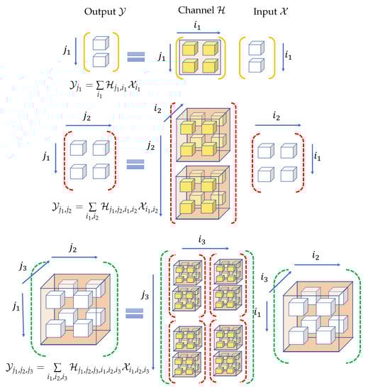
Figure 1.
The tensor system model and its evolution with the increase in order.
2.2. Examples of Practical Systems
A few examples of domains that may exist in a system include space, time, frequency, users, spreading sequence, channel multipath, and device index. Incorporating any additional domain of transmission in the unified system model can be carried out in an intuitive and comprehensible manner using the tensor framework. For instance, it is shown in [19] that a MIMO Orthogonal Frequency Division Multiplexing (OFDM) system can be represented using order 2 input and output tensors where both antenna and sub-carrier domains are considered. Thereby, the effective channel can be represented using an order 4 tensor with its domains corresponding to receive antenna, receive sub-carrier, transmit antenna, and transmit sub-carrier. The output is then given using (3) where the Einstein product is taken over the two transmit modes between the channel and the input. Such a representation allows us to jointly consider both inter-carrier and inter-antenna interference in a single framework. Similarly, a MIMO Filter Bank multi-carrier (FBMC) system can also be represented using order 2 input and output tensors and an order 4 channel tensor where the antenna and sub-carrier domains are considered [9].
The system model can further be used for Generalized Frequency Division Multiplexing (GFDM) as well. GFDM is a flexible filtered multi-carrier modulation scheme where out of band radiation of the transmit signal is controlled using pulse shaping filters on each sub-carrier. GFDM uses a block-based transmission scheme where data symbols are transmitted over a time–frequency block having K sub-carriers and M timeslots called sub-symbols [23]. The traditional OFDM can be seen as a special case of GFDM when and the modulator matrix is a DFT matrix. GFDM can also be seen as a generalization of single carrier FDM under suitable pulse shaping filter options [23]. Since GFDM is a generalization of other FDM schemes, it is called ‘Generalized’ FDM. A detailed comparison of GFDM with OFDM and single carrier FDM can be found in [24].
For single antenna transmission, since components in each GFDM transmit block have separate dependence on the sub-carrier and sub-symbol indices, it is more convenient to represent the data symbols using an order 2 tensor of size . Further, in a MIMO GFDM system, the input and output can be represented as order 3 tensors indexed by antenna/stream, sub-carrier, and sub-symbol indices. Consider a MIMO GFDM system where S independent streams of data are transmitting data symbols each. The transmit data symbols can be arranged in an order 3 tensor where corresponds to the complex symbol on the kth sub-carrier, mth sub-symbol, and sth transmit stream. Similarly the received signal and noise tensors can be represented using third order tensors and . Subsequently, the channel that couples the input with the output can be seen as an order 6 tensor . Let and denote the number of transmit and receive antennas, respectively. The tensor channel considered here is the equivalent channel obtained from the cascading of the transmit filter tensor , physical channel , and the receive filter tensor , i.e., . The overall system model is represented using (3) as
A detailed derivation of this system model for MIMO GFDM along with characterization of and can be found in [25]. The model in (4) shows the innate ability of the tensor framework from (3) to incorporate additional domains in the system model.
In addition to spatial, temporal, and frequency domains, different users can also be considered as a domain in the system model. Consider the uplink of a multi-user MIMO system where a base station (BS) equipped with antennas is receiving information from K users, each having antennas. Using the standard matrix notation, the received signal vector at the base station can be written as
where is the signal transmitted by the kth user, is the received noise vector, and is the channel matrix between the kth user and the BS. Such a system can be equivalently represented in the tensor framework using a third order channel tensor. We define the multi-user MIMO tensor channel as an order 3 tensor where each forms a slice of the third order tensor as . The input signal can be defined as an order 2 tensor , where each forms a column of the matrix . Hence, the system model in (5) can be equivalently represented as:
Furthermore, in cellular networks, the notion of domains in the system model can be expanded to include the cell index as well. In such a case, the channel tensor will incorporate terms corresponding to the inter-cell interference also. Consider a K cell MIMO interfering broadcast channel (IBC) as in [26], where each cell consists of a base station with M antennas and U users with L antennas each. The channel matrix between the kth base station to the uth user in the ith cell is denoted by a matrix . Let be the broadcast transmitted signal vector by the kth base station intended to be received by all the users within its cell. Then, the received signal vector at the uth user in the ith cell is given as [26]:
where denotes additive noise vector for the uth user in the ith cell. Note that the summation in (7) includes the desired term (corresponding to ), and also the interference terms received by a user from a base station outside its cell (inter-cell interference corresponding to ). The system model in (7) can be represented using the tensor framework from (3). Consider the transmit signal corresponding to K base stations, each with M antennas as an order 2 tensor , where each vector forms a column of the matrix . Similarly, the output and noise received by U users in each of the K cells with L antennas per user can be defined as order 3 tensors and , respectively such that and . The channel can subsequently be defined as an order 5 tensor such that . Thus, the system model from (7) can be equivalently written using the Einstein product as:
Other examples of using tensors to represent multi-domain signals can be found in the literature. For example, a Direct-Sequence Code Division Multiple Access (DS-CDMA) system [11] uses an order 3 tensor for signal representation accounting for antenna, temporal and spreading domains. Furthermore, [12] represents the signals using order 5 tensors in a MIMO OFDM CDMA system with antenna, data streams, sub-carriers, time blocks, and chips as the domains. Multi-domain index modulation as advocated in [27], uses transmission over spatial, temporal, frequency, coding, as well as a hybrid combination of such domains to exploit all the indices of transmit resources. Thus tensors are an effective tool for multi-domain signal representation.
Note that several such multi-domain communication systems can also be represented using a degenerate setup employing vectors and matrices. The signals corresponding to different domains can be concatenated to be represented as vectors, and the channel can be modeled as a matrix. Since multiple indices of signals are collapsed into a single index using such concatenations, it leads to a cluttered and not an intuitive system model. The ease of representation through the tensor framework becomes even more prominent as the number of domains required to be incorporated in the system model increases. Furthermore, since the tensor representation preserves the structure of the signals, it helps in developing signal processing schemes which harness the structural properties of the signals. In addition, there can be cases where signals or data are represented as tensors for storage efficiency using the Tensor Train (TT) format [28], thereby restricting the flexibility to reshape the tensors into a vector or matrix. We elaborate on such advantages of the tensor formulation in the next section. We present some signal processing techniques that make use of various tools from multi-linear algebra to simultaneously exploit all the domains that exist within a communication system.
3. Simultaneous Signal Processing Across Domains
Signals and systems representation using tensors leads to the notion of tensor-based multi-domain filtering. The structure of the tensor plays a key role in such operations. A square tensor is an even order tensor of order where the dimensions of the first N domains are the same as that of the last N domains. A square tensor of size , whose elements are indexed by variables , is called pseudo-diagonal if non-zero elements occur only when . Note that this structure is different from a diagonal tensor, where non-zero elements only occur when all the indices are equal. Hence, diagonal elements are a subset of the pseudo-diagonal elements. An illustration of the pseudo-diagonal elements of a fourth order tensor is presented in Figure 2. The green blocks, where and , are the pseudo-diagonal elements. The diagonal elements, where , are represented by green blocks marked with a white X. More details on pseudo-diagonal tensors can be found in [9]. An identity tensor denoted as is a pseudo-diagonal tensor with all non-zero entries being 1. The pseudo-diagonal structure helps us classify TPRS and understand its spectrum and cross-spectrum shaping capabilities, as discussed in the next sub-section. As a precursor to TPRS, we first explain the notion of spectrum and cross-spectrum in tensor framework.
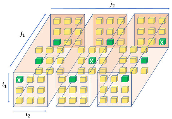
Figure 2.
Pseudo-diagonal elements of a tensor of size .
Consider a tensor sequence which is a function tensor with discrete argument k. The D transform of is a tensor function defined as:
with components , where D is the delay operator.
A tensor is said to be random if its components are random variables. Similarly, a tensor sequence is called a random tensor sequence if its components are random processes indexed by variable k. The expected value (mean) of such a tensor sequence is defined as where . In addition, the auto-correlation of the tensor sequence denoted as is defined as an order function tensor where each component is a function of two discrete variables k and i. It can be described using the outer product as:
which can be written component wise as:
where denotes complex conjugate. Subsequently, a tensor sequence is called wide sense stationary (WSS) if its mean is independent of k and its auto-correlation depends only on i. The spectrum tensor of a WSS is an order tensor function where each component is a function of the variable . The D transform of the auto-correlation is given as:
and the spectrum tensor is defined as:
where T is the tensor symbol interval. Thus, the spectrum tensor corresponding to is a tensor function of order whose pseudo-diagonal elements are the spectrum of each component of and the off pseudo-diagonal elements are the cross-spectrum between two different components and .
3.1. Tensor Partial Response Signaling
Correlative coding, otherwise known as Partial Response Signaling, is a transmission method where correlation is introduced between successive symbols through the addition of a controlled amount of inter-symbol interference [29]. The objective is to shape the spectrum of the signal using correlative codes to achieve desirable properties. Frequency domain correlative coding has been also applied in MIMO OFDM systems to mitigate the effects of time-selective fading [30].
In such a system, the correlation introduced is restricted to one domain. Using the tensor framework, it is possible to extend this concept to a multi-domain system and control both the spectrum as well as the cross-spectrum of the transmitted signal tensor. Such a method, dubbed Tensor Partial Response Signaling (TPRS), makes use of tensor correlative codes to introduce a controlled amount of inter-tensor interference (between successive tensor symbols) and intra-tensor interference (between the domains of one tensor symbol).
Consider a WSS discrete sequence of zero mean uncorrelated data tensors with the corresponding as an identity tensor of order . To introduce correlation and alter the input spectrum tensor, we pass through a linear discrete time invariant system . Hence, the output of the system, denoted by is given using discrete contracted convolution between and , defined as [9]:
which in the D transform domain can be written as:
The objective of is to introduce correlation in the transmitted data tensor; hence, we refer to as a TPRS system. Since the data tensor sequence is assumed WSS, we can relate the tensor to by:
A detailed derivation of (16) can be found in [31]. The relation in (16) when evaluated at shows that the spectrum tensor of the transmit data tensor can be manipulated to alter both the spectrum and the cross spectrum among all the components by suitably changing the structure of the TPRS system . The data streams in most digital communication systems consist of independent and identically distributed (i.i.d) symbols drawn from a specific constellation, implying that such sequences have a flat spectrum. For a tensor system with data tensors whose components are i.i.d, all components of the spectrum are the same. The cross-spectrum is zero as the individual components are not correlated, making a multiple of identity tensor. In this case, (16) reduces to . Hence, by using a TPRS system, it is possible to shape the spectrum and cross-spectrum of the different components of the data tensor by employing distinct codes. This means that the components of the transmitted signal tensor can have different spectral shapes even though the original data tensor has components that are i.i.d.
Depending on how the interference is introduced, TPRS systems can be broadly classified into different classes. Controlled interference from within the same tensor symbol (intra-tensor interference) changes the level of the spectrum and cross-spectrum while maintaining a flat spectral power density. Such systems are dubbed Degenerate TPRS systems and are used in multi-carrier transmission schemes where some inter-carrier interference is allowed in order to achieve better error performance without compromising the spectral efficiency of the overall system [30]. On the other hand, pseudo-diagonal TPRS systems contain controlled interference from successive data tensors (inter-tensor interference) only and can be used to change the shape of the spectrum and cross-spectrum of the transmitted signal tensor. When combining these two classes of TPRS systems it is possible to create spectrum tensors where certain components have a desired spectral shape while others have a flat spectrum at a desired height.
In Figure 3 and Figure 4, we illustrate the spectral components of transmitted signal tensor for two different cases. The transmitted signal is a matrix and the corresponding spectrum tensor is of size . Each box in Figure 3 and Figure 4 corresponds to a particular component of the transmitted signal tensor denoted by the row and column indices . The x-axis labeled as index in the figures represents the indices corresponding to the components of the spectrum tensor, the y-axis labeled as represents the angular frequency, and the z-axis labeled as represents the spectrum magnitude. The green line represents the spectrum of component and other colors represent the cross-spectrum between and another component of the transmitted signal. For example, the shape at index represents the cross-spectrum between component and of the matrix. The degenerate TPRS system contains only intra-tensor interference. Hence, all the components of the spectrum tensor are flat. In contrast, for TPRS with both inter- and intra-tensor interference, the spectral components have different shapes due to the addition of controlled inter-tensor interference. The corresponding correlative codes for Figure 3 and Figure 4 are included in Table 2. The TPRS system for these examples is an order 4 tensor , where each component corresponding to Figure 3 and Figure 4, is listed in the second and third columns of Table 2, respectively.
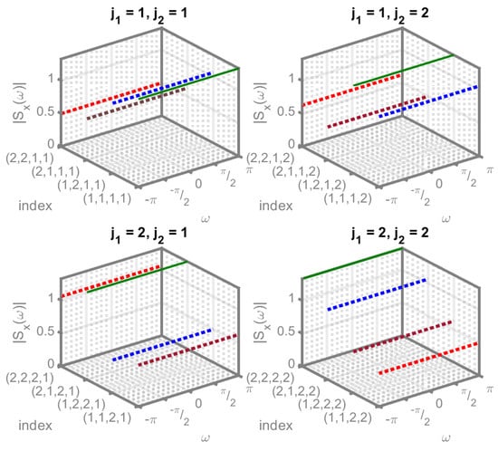
Figure 3.
Degenerate TPRS.
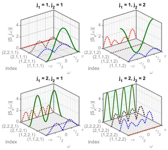
Figure 4.
TPRS with inter- and intra-tensor interference.
Table 2.
Structure of the TPRS system.
3.2. Tensor-Based Receiver Designs
Tensor equalization has been considered in [9] as a technique of reducing interference in multi-domain communication systems. In particular, [9] presents multi-linear minimum mean square error (MMSE) and zero forcing equalizers, while [31] also presents tensor-based decision feedback equalizers. Such techniques can be used to design receivers which simultaneously combat the effects of interference from different domains (Multi-Domain Interference) such as inter-carrier interference (ICI), inter-symbol interference (ISI), inter-antenna interference (IAI), and inter-user interference (IUI). An application of such a tensor-based equalizer in a multi-user MIMO GFDM receiver is considered in [9], where it is shown that such tensor-based equalizers outperform the per-domain equalizers which do not exploit the information on interfering terms from other domains.
The tensor framework can also be used to develop estimation techniques for receiver design in communication systems. In (3), if the channel tensor is known, a multi-linear receiver which operates on the received signal tensor producing , can be used to provide an estimate of the transmitted tensor . We can find the tensor such that the mean square error between and , defined as
is minimized. The notation denotes Frobenius norm. This leads to a tensor multi-linear MMSE receiver which is specified by:
where and are order and covariance tensors of input and noise, respectively (assuming that and are zero mean). A detailed derivation of (18) can be found in [19]. An application of such a tensor-based receiver in a MIMO OFDM system is considered in [10] where a comparison with per sub-carrier estimation which ignores the inter-carrier interference terms for estimation is presented. It is shown that as interference from other sub-carriers becomes dominant, the performance of per sub-carrier receiver deteriorates significantly, while the tensor receiver’s is significantly better since it makes use of the interference terms for data estimation.
3.2.1. Complexity of Tensor Multi-Linear MMSE Receiver
The process of finding the multi-linear MMSE operator using (18) involves performing the Einstein product and tensor inversion. We now assess the computational complexity of finding . We refer to a single floating point operation (addition, subtraction, multiplication, or division) as a flop. For simplicity of explanation, we assume the channel to be a square tensor, i.e., and . The Einstein product between two tensors of size each requires flops [19]. Note that if the number of flops required for any step is polynomial in variable n, we state the complexity as where p is the degree of the polynomial. The process of calculating can be broken down into sequential steps which are listed in Table 3 along with the computational cost of each step.
Table 3.
Computational complexity of a tensor multi-linear MMSE receiver.
The first step in Table 3 is calculating two Einstein products; hence, its complexity is . The next step performs an element-wise addition of two tensors with elements in each; hence, it requires operations. Note that in several cases where the noise tensor contains uncorrelated elements, the noise covariance will be a pseudo-diagonal tensor. In such a case, the number of non-zero elements in the noise covariance tensor would be ; hence, the cost of this step would become . Further, the next step calculates the inverse of an order tensor. Tensor inverse can be calculated using the Newton’s method which solves an iterative equation involving the Einstein product with a complexity of as described in [10]. The final step again requires two Einstein products, and therefore has a complexity of . If we add all the complexities in Table 3, we see that finding requires an overall operations, which is cubic in the number of input/output tensor elements, . It is to be noted that many of these operations can be computed using parallel processors to significantly reduce the time complexity of executing them. A detailed description of parallel and faster implementation of the Einstein product and the tensor inversion using Newton’s method can be found in ([10] Appendix D). Several other algorithms to compute tensor inverse, without any need of tensor transformation to matrix or vector, have been considered in literature [15,16] which rely on the Einstein product. For instance, [15] presents a higher order bi-conjugate gradient method, and [16] presents an elimination method using tensor triangular decompositions.
3.2.2. Application of Tensor Train Decomposition and Tensor Networks
Algorithms which allow to perform various tensor operations without reshaping the tensors provide an important feature as matrix or vector transformation of the tensors is not desirable in many applications. Very often, large data are stored using Tensor Train (TT) decomposition for reducing storage complexity [28,32]. In TT format, a higher order tensor is written in terms of a set of sparsely connected lower order tensors called cores. For a tensor of size , the TT decomposition is specified by:
where each core is a third order tensor of size and denote the TT ranks with and for [28]. Since the TT ranks determine the storage consumption of the tensor, the structure of the core tensors with low TT ranks is exploited for reducing the storage complexity. In such a process, rather than storing the entire tensor, only the tensor cores along with the information on the modes to be contracted are stored. Hence, any mathematical operation to be performed on the tensor should be able to act on the cores itself without reconstructing the entire tensor. This restricts any reshaping of the data. A tensor in TT format can be graphically represented through a Tensor Network (TN) containing nodes and edges [32]. Each core is represented by a node, and a contraction between two cores is represented by connecting the nodes through an edge. The free edges emerging from a core correspond to the modes which are not contracted. Any mathematical computation between two tensors can be expressed in terms of their TNs. For instance, contracted product between two different tensors can be achieved using TNs by connecting the free edges corresponding to the modes to be contracted of the two tensors. A detailed description and examples of different tensor operations using TN representation is provided in [32]. Consider the system model presented for order 3 input output tensors and order 6 channel tensors in Figure 1. A TN representation of this model is illustrated in Figure 5. It shows the representation of the Einstein product between the third order input and the sixth order channel in TT format. The operation can be written in terms of the cores of and as
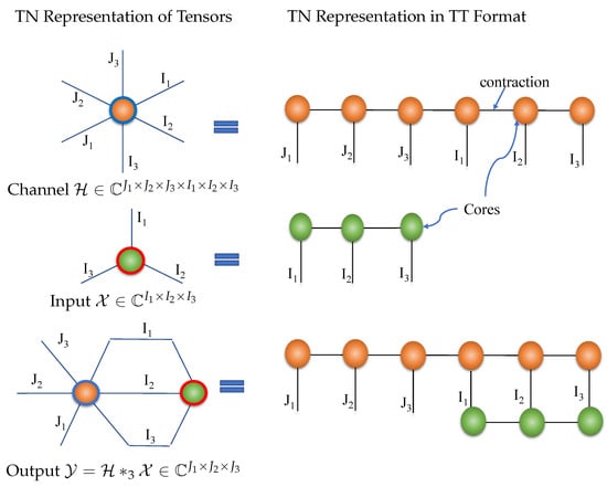
Figure 5.
TN representation of a multi-domain communication system model with sixth order channel tensor.
The summation over indices in (20) is reflected in the edges connecting the green and the orange nodes in Figure 5. Specific algorithms to compute the Einstein product, which act directly on the cores of the tensor train format are presented in [33].
More recently, the concept of tensor networks has been also considered for developing error-correcting codes such as a generalization of polar codes. The notion of polar codes was first introduced in [34] as a class of capacity-achieving codes for binary memoryless symmetric channels. The use of such channel codes can significantly enhance the transmission reliability of wireless communication systems. Hence, polar codes have found applications for channel coding in 5G wireless systems [35]. A family of codes, known as branching MERA codes, developed using tensor networks and tensor contraction which generalizes polar codes, has been presented in [36]. Essentially, the encoding sub-system is represented as an even order tensor. At the receiver, the sequential cancellation decoding operation is modeled as a contraction that is represented by a TN. Further, [36] shows that such a generalization of polar codes using TN outperforms traditional polar codes in its error-correcting ability. Another generalization is presented in [37] which develops the decoding algorithm using TN for polar and convolutional polar codes. The use of tensor formalism for the development of error-correcting encoding and decoding algorithms emerges as a novel and interesting research trend that integrates tensors and channel coding for communication systems.
3.2.3. Applications of Other Tensor Decompositions
A receiver based on (18) assumes that the channel is known. However, even in the absence of complete channel state information, the structure of the received signal can be exploited through several tensor decomposition schemes for designing blind/semi-blind receivers [11,12,14]. Such receivers can perform joint symbol and channel estimation. In fact, one of the initial applications of tensors for wireless communication signal processing was considered in [11] for a blind receiver design where the signal in a DS-CDMA system is modeled as a third order tensor. Information is extracted from the received signal using tensor canonical polyadic (CP) decomposition, also known as parallel factors (PARAFAC) decomposition. The CP decomposition breaks a tensor into a linear combination of rank one tensors. By making use of the uniqueness of the three-way PARAFAC decomposition, ref. [11] presents a blind receiver for user separation, equalization, and detection in a DS-CDMA system. The work in [11] and several other blind receiver design schemes rely on the uniqueness of the PARAFAC decomposition of third order tensors, and therefore cannot be accomplished in a degenerate setting comprising vector or matrix formulations. Another common tensor tool is the Tucker decomposition which has primary applications in finding low rank structures, classification, and feature extraction in high dimension data [32,38]. Some suitable variations of PARAFAC and Tucker decompositions lead to the development of many related tensor decompositions which can be used to model signals and develop coding techniques in multi-antenna communication systems as shown in [12,13] and references within. For instance, a tensor space–time–frequency coding technique for a MIMO OFDM CDMA system is developed in [12], where the coding tensor is represented using a fifth order tensor. The baseband equivalent received signal is also represented as a fifth order tensor which under some suitable assumptions on the channel admits a generalized PARATUCK (a combination of PARAFAC and Tucker) model. Based on this model, semi-blind receivers are then used for joint symbol and channel estimation. A short summary of a few of the important tensor tools along with some applications can be found in Table 4. More details on various tensor decompositions and their numerous applications can be found in [14,21,38,39]. A tensor singular value decomposition (SVD) is described in [15] which decomposes a tensor into two unitary tensors and a pseudo-diagonal tensor connected via the Einstein product. Note that both PARAFAC and Tucker decompositions can equivalently be represented using the Einstein product-based tensor SVD if the components of the unitary tensors are obtained using a product of the elements of the factor matrices in PARAFAC and Tucker decompositions as described in ([15] Lemma 3.20 and 3.22).
Table 4.
Tensor tools and applications.
All such tensor-based receiver designs rely on exploiting the received signal structure by simultaneously processing multiple domains. Simultaneous signal processing across domains reveals the trade-off between these domains, which can be used for efficient resource utilization, as discussed in the next section.
4. Harnessing the Domain Trade-Off
The trade-off between domains in a communication system can be explored through an information theoretic analysis of the tensor channel from (3) which is presented next.
4.1. Capacity of a Tensor Channel
The MIMO matrix channel can be decomposed into parallel non-interfering scalar channels using matrix eigenvalue decomposition (EVD). The optimum input power allocation is done by the classical water-filling solution applied to the decomposed parallel channels to achieve capacity [43]. The unitary matrix obtained from the channel EVD is used to prescribe a transmit precoding. However, these power allocation and precoding operations are restricted to the transformation of transmit vectors in the antenna domain only. The tensor framework extends these operations to multiple domains.
For the system model defined in (3), assuming and are zero mean independent and the channel tensor is known, the covariance tensor of the output denoted as can be written as:
where and are the input and noise covariance tensors, respectively. Assuming the noise tensor contains circular symmetric zero mean complex Gaussian entries with covariance tensor as identity, i.e., , it can be shown (using ([25] Lemma 1)) that the mutual information between input and output tensors satisfies:
where equality is achieved only if is Gaussian. Here we consider log to the base 2, and the det(.) operation is the tensor determinant of the enclosed entity, defined as the product of the tensor eigenvalues [16]. For a fixed channel, it can be shown that in the presence of zero mean circular symmetric Gaussian noise, the output from (3) will also be zero mean circular symmetric complex Gaussian if is so. Hence, for maximizing the mutual information, we consider to be circular complex Gaussian with covariance . The capacity of the tensor channel can be then found through the following convex optimization problem:
where denotes the sum of the pseudo-diagonal elements of . The inequality constraint represents a sum power constraint on the input, and means that the input covariance tensor is positive semi-definite. Such an optimization problem and can be solved using the Karush–Kuhn–Tucker (KKT) conditions resulting in the optimal input covariance and the capacity as:
More details on the derivation of (24) and (25) can be found in [25]. The unitary tensor and the pseudo-diagonal tensor are obtained from the tensor EVD of , given as . Such decomposition can be computed using tensor EVD methods presented in [15,16,17]. The eigenvalues of which are the pseudo-diagonal elements of are denoted by . The constant is chosen to satisfy the power constraints, and indicates that each element in the enclosed entity is non-negative, i.e., .
The solution in (24) can be seen as a higher order generalization of the classical water-filling solution for the MIMO channel to a tensor setting. Assigning the optimum covariance tensor to the input performs power allocation across all the domains and also prescribes a multi-domain input precoding strategy. Notice that the eigenvalues of depend on the multitude of domains in the tensor channel. This paves the way for certain flexibility to exploit the trade-off between different domains, depending on the specific tensor channel eigenvalues. The capacity is obtained by summation of a log function over all such multi-domain eigenvalues. The lack of resources in a specific domain can be compensated with resources in alternate domains, which would allow a more judicious and efficient resource allocation mechanism. In the next section, we elaborate on such a domain trade-off through numerical examples.
4.2. Numerical Examples
We find the capacity of a tensor channel with i.i.d zero mean and unit variance circular complex Gaussian entries, under total power constraint. We assume that the channel realizations are known at the transmitter and receiver. The results presented are averaged over 100 different channel realizations. Furthermore, we assume additive white Gaussian noise (AWGN) with zero mean. The signal to noise ratio (SNR) is defined as the ratio of the transmit power to the noise variance. Capacity is calculated at 8 dB SNR using (25). Both input and output are order 2 tensors of size each, where X and Y denote the dimensions of the individual domains. Thereby the channel is a fourth order tensor of size . Figure 6 presents the capacity of such a fourth order tensor channel against X and Y. As X and Y increase, the capacity of the tensor channel increases. It can be further observed that different configurations of X and Y can achieve same capacity, allowing a trade-off between available resources in the two domains. For instance, an input and output tensor of all achieve the same capacity. Each line curve on the surface plot in Figure 6 represents different configurations of which achieve similar capacity. The design of any multi-domain communication system needs to consider the restrictions on the size of individual domains due to bandwidth or antenna limitations or other domains specific constraints.
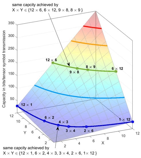
Figure 6.
Capacity vs. dimensions of order two input and output tensors.
The domain trade-off is further apparent in Figure 7 which illustrates the behavior of the capacity under sum-power constraint against SNR. The transmitter employs a vector input, i.e., a single domain of dimension 8 and the output is a tensor of various number of domains. The channel capacity curves show an increase in the capacity achieved when the number of receive domains is increased. It can also be observed that the capacity achieved by an channel is the same as that of the capacity achieved by an channel. This implies that even with limited resources in one domain, increasing the number of domains can give higher capacity by exploiting the trade-off between multiple domains.
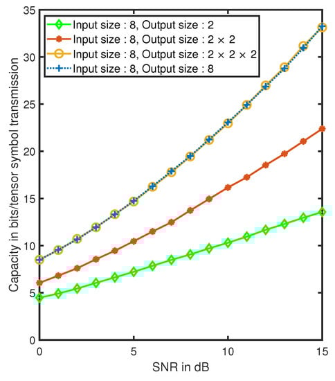
Figure 7.
Capacity vs. SNR for different domain configurations at the receiver.
Similar trade-off can be observed between domains in the mean square error (MSE) performance at the receiver when joint signal processing is performed across all the domains using the tensor multi-linear MMSE approach. Figure 8 shows the MSE results for different configurations of input and output. The transmit tensor has i.i.d. components drawn from a 4-QAM constellation with unit energy such that the transmit covariance is a scaled identity tensor , with . The channel entries are i.i.d zero mean unit variance circular complex Gaussian. Further, the channel is normalized to make the average received signal power the same as the total transmit power , where denotes the number of elements in the transmit tensor. We assume the noise tensor has i.i.d. zero mean and variance circular complex Gaussian entries. Since the channel is normalized to provide unit power gain, the signal to noise ratio is defined as , where denotes the number of elements in the output tensor. A tensor-based multi-linear MMSE receiver from (18) is employed to estimate the transmitted signal. With input and its estimate , the normalized mean square error is defined as MSE = . The plotted results are averaged over 100 different channel realizations, with 500 different noise and input realizations for each channel. The input has a single domain of dimension 8, and output has a variable number of domains. It can be observed that better MSE performance is achieved as the number of domains at the receiver is increased. When the output has a single domain of dimension 2, the MSE is fairly high as the number of elements in the output are far less than the number of transmit elements. As the number of domains at the receiver increases, we get better MSE performance. Further, the performance of a system with three domains of dimension 2 at the receiver is the same as the performance of a system with a single domain of dimension 8 at the receiver. Hence, performance improvements can be achieved by addition of domains rather than having to increase the dimensions of individual domains. Such domain trade-off is exploited through the tensor multi-linear MMSE receiver which jointly estimates the signal across all the domains.
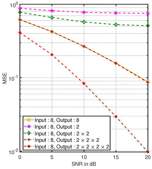
Figure 8.
MSE vs. SNR for different domain configurations at the receiver.
So far in these examples, we have observed that the individual domain’s dimensions can be flexibly interchanged if the overall size of input and output remains constant. However, it is important to note that such a behavior is observed over an average of 100 iterations when all the tensor channel entries are i.i.d. Gaussian, which has been the case in our numerical examples so far. For any two given channel tensors with the same overall size but different dimensions of individual domains, the capacity may not always be exactly same. The exact nature of such a domain trade-off would depend on the specific tensor channel eigenvalues. The example of a channel with i.i.d. Gaussian entries without tagging specific physical meaning to the domains incorporated was put forward only to illustrate the basic idea of trade-off. Further, to understand such trade-off in a more realistic set-up, we consider the example of a MIMO GFDM system from (4), where the channel is represented as an order 6 tensor of size . The system model follows the representation from (4) in Section 2.2. The model is further illustrated in Figure 9, where order 3 tensors are denoted using cubes and higher order tensors are denoted using double edge squares with the order mentioned on top right corner.
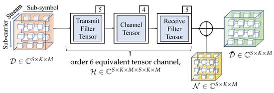
Figure 9.
Tensor system model for MIMO GFDM.
Let the number of transmit and receive antennas be and , respectively, with . Such an order 6 tensor channel associated with MIMO GFDM is considered in [25], where capacity behavior with respect to the different pulse shaping filter options is explored. Here, we use the simulation set-up from [25] and analyze the capacity for different number of data streams, sub-carriers, and sub-symbols, denoted by and M, respectively, to explore the trade-off between these domains. The channel is generated as a cascade of transmit filter, physical channel and receive filter. In this example, we use a raised cosine transmit pulse shaping filter with roll off factor 1 at the transmitter. The receive filter is matched to the transmit filter and the entries of the physical channel are generated using i.i.d. complex Gaussian with zero mean and unit variance. Furthermore, the entries of the equivalent channel are normalized to ensure that the average received power is same as the transmit power P. The noise tensor contains zero mean and unit variance circular symmetric Gaussian entries such that noise covariance is with . With channel gain normalized to one, the signal to noise ratio is defined as [44], where is the transmit energy per element defined as . We assume that is known at the receiver and the transmitter. The tensor framework gives us the capacity in bits/tensor symbol, where in this case a tensor symbol contains elements across all the sub-carriers, sub-symbols, and antennas. Hence, we normalize the capacity of the MIMO GFDM channel by the number of sub-carriers and sub-symbols as in [25,44]. Figure 10 shows the normalized capacity against SNR for different values of and M. It can be seen that for a fixed value of , as S increases we get higher capacity. In addition, for a fixed S, choosing different configurations of K and M, such that the product is constant, leads to almost similar capacity results. The capacity when is almost the same as the capacity with , and slightly lower than with . This exhibits the latent trade-off between the sub-carrier and sub-symbol domains, which can be harnessed using the tensor framework.
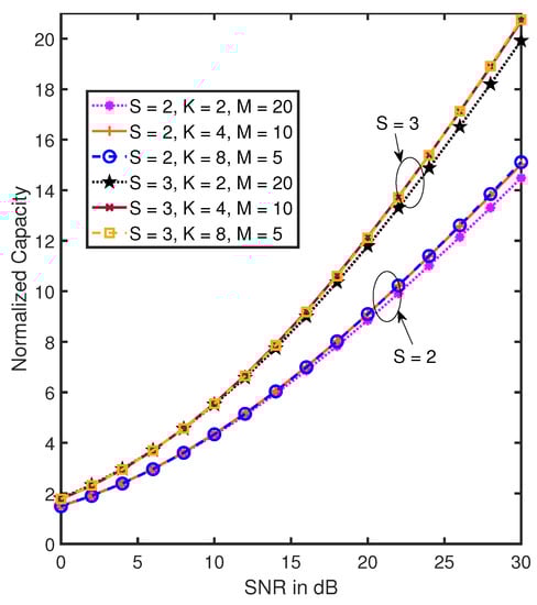
Figure 10.
Capacity vs. SNR for MIMO GFDM.
A domain trade-off can exist in many multi-domain communication systems. Another specific example of domain trade-off is presented in [45] which considers a layered maximum likelihood detection scheme for MIMO systems. Assuming a frequency selective fading channel, [45] considers a multipath component in every transmit–receive antenna pair as a virtual transmit antenna. Hence, the word ‘layer’ is used for the group of virtual antennas transmitting the same stream of data in its actual and delayed versions. The transmit signal is represented using a matrix (order 2 tensor) with domains corresponding to antennas and delay. Further, [45] uses over-sampling at the receiver which increases the dimension of the received signal to compensate for the lack of antennas, and thereby represents the output also as a matrix (order 2 tensor) corresponding to time and space domains. Thus, by harnessing the trade-off between the space and time domains at both the input and the output, [45] develops a maximum likelihood receiver for a MIMO OFDM system, which leads to an improved error rate performance.
4.3. Multi-Domain Beamforming (Precoding)
Assigning the optimal covariance to the input based on (24) can be seen as comprising of two parts: power allocation and transmit precoding. It performs a multi-domain power allocation using tensor water-filling based on the pseudo-diagonal tensor . It also performs transmit precoding using the unitary tensor to multi-linearly transform the input signal. The tensors and are essentially the pseudo-diagonal and the unitary tensors in the tensor EVD of the optimal covariance, respectively. Assume an input tensor which has zero mean unit variance i.i.d elements. To generate the transformed input tensor with the optimal covariance given by (24), we perform:
where denotes the square root of a tensor [46]. For a pseudo-diagonal tensor with real non-negative elements, the square root is simply an element wise square root. Since has zero mean and identity covariance tensor, it can be readily verified that the covariance of from (26) is indeed given by (24).
The unitary tensor is obtained via the tensor EVD of , and it is the same as the right unitary tensor obtained from the tensor singular value decomposition (SVD) of . For details on tensor SVD, please refer to [15,47]. The multi-linear transformation of the input through the tensor can be seen as multi-domain beamforming, where is the beamformer tensor. The traditional beamforming approach makes use of the unitary matrix from MIMO matrix channel SVD which leads to beamforming in spatial (antenna) domain only, and hence can be seen as single domain beamforming. Multi-domain beamforming, which results naturally in the tensor framework, extends this operation to be performed jointly across all the transmission domains. For instance, consider the MIMO GFDM system from (4). The multi-domain beamformer will be obtained by solving for optimal input covariance which achieves the capacity of the MIMO GFDM equivalent channel . Thus, the beamforming tensor operates across all the spatial, temporal, and frequency domains and accounts for not just the physical channel but also the transmit and receive filter parameters. The choice of the optimal covariance depends on the power constraint at the input. Under a sum-power constraint, the solution is given by (24). However, in a practical system we may have constraints on each transmit antenna [48]. Such per antenna power constraints can be naturally accounted for in the tensor framework.
In a practical MIMO system, each antenna may be connected to a separate power amplifier with finite dynamic range on the individual RF chain, creating the need for per antenna power constraints. Another scenario where such constraints are common is distributed MIMO which has transmit antennas located at different physical locations that do not share the same power source [48]. Hence, in a MIMO system, per antenna power constraints rather than a sum-power constraint is an important consideration which is of practical interest [48,49]. Consider a MIMO GFDM system represented by (4) with 2 transmit and receive antennas. For simplicity of explanation, we assume . Rather than a sum-power constraint P on the entire input symbol, we may have different power budgets and for the transmit antennas separately. In a MIMO system model where the input is a vector corresponding to a single domain (antenna), this constraint becomes a per element power constraint on the input vector. However, in a multi-domain system such as MIMO GFDM, corresponding to each antenna we have data symbols over K sub-carriers and M sub-symbols. The tensor framework defines the input as a third order tensor, and thereby its covariance as a sixth order tensor . Hence, the per antenna power constraints can be defined as a set of constraints on the pseudo-diagonal elements of the covariance:
Subsequently, finding the optimal covariance with per antenna power constraints to achieve capacity requires finding a positive semi-definite covariance tensor subject to (27) such that is maximized. Since the constraints from (27) are linear, finding the optimal still remains a convex optimization problem that can be solved using the KKT conditions. Such solution yields a multi-domain beamformer with per antenna power constraints.
Several beamforming techniques are suggested in [50] for MIMO GFDM systems using matrix SVD. The system model in [50] combines all the domains of transmission to form vectorized signals, and represents the channel using a matrix. Using such a model, ref. [50] suggests a scheme where beamforming is performed after GFDM modulation. The input, which is represented as a vector with symbols, is first modulated using a modulator matrix and then multiplied by a transmit beamforming matrix to generate the transmit vector as across all the transmit antennas. The model implicitly assumes that the same GFDM modulator matrix is used for all the antennas. The beamforming matrix is chosen based on the SVD of the matrix channel , where represents the channel between the output of the GFDM modulator and the received signal. Another scheme presented in [50] performs the beamforming before the GFDM modulator, thereby accounting for not just the physical channel but also the modulator matrix. In this scheme, the modulator matrix is defined as a block diagonal matrix where main diagonal blocks are . The input is generated using the beamformer matrix as , where the matrix is obtained using the SVD of matrix . In addition, a sub-optimal scheme presented in [50] considers single antenna selection for transmission without any beamforming across the sub-carriers and sub-symbols. The antenna selection is done such that the received SNR is maximized. The transmit beamformer matrix corresponding to the antenna selected is an identity matrix of size , denoted by , and for every other antenna it is an all zero matrix of size , denoted by . Hence, the structure of the beamformer matrix is given as , and the transmit signal is generated as . This can be seen as single domain degenerate beamforming.
The first two beamforming techniques presented in [50] can also be seen as multi-domain beamforming albeit in a vector/matrix framework. These account for all the domains of transmission by concatenating the input signals across various domains to form a vectorized input. Hence, as far as finding the beamforming operation under a sum-power constraint is concerned, the vectorized approach is conceptually equivalent to the tensor approach. However, under practical constraints such as per antenna power constraints, the tensor model has a significant advantage over the vectorized model. In the vectorized input signal various indices corresponding to all the antennas, sub-carriers, and sub-symbols have been reduced to a single index. This makes the incorporation of any per domain constraints difficult and not intuitive, as the domains are not separated by different indices. On the other hand, the tensor model allows to keep the structure of the channel and the input/output intact, and thus can easily incorporate practical constraints which are domain specific, as in (27), while designing the transceiver schemes. The proposed tensor framework is intuitive and flexible, allowing for convenient incorporation of such power constraints for any number of antennas, and even extend the constraints to per sub-carrier or per sub-symbol in MIMO GFDM or per user in a multi-user system.
5. Conclusions
This paper presents a tensor-based perspective on multi-domain communication systems. Multi-domain communication systems can be considered as an evolution of MIMO where the presented tensor framework leads to the exploitation of not only the space domain through multiple antennas, but also joint use of various other domains. A generic system model where the input and output are represented using tensors, which are linked through a tensor multi-linear channel using the Einstein product, was presented. The proposed system model can be used to model many practical communication systems. As a demonstration of the use of our framework for multi-domain signal processing in communication systems, we considered the notion of TPRS which allows the introduction of controlled inter-domain interference for shaping the spectrum and cross-spectrum of multi-domain signals. Further tensor-based multi-linear MMSE detection, which utilizes the interference terms for joint data estimation across all the domains, was also presented. It was shown that for a fixed transmit tensor, better MSE performance is achieved with an increase in the number of receive domains. In addition, the tensor framework is best suited to unravel the latent trade-off that exists among domains. This was illustrated through an information theoretic analysis of the tensor channel. We presented numerical examples demonstrating the domain trade-off benefits in the capacity and mean square error performance. It was shown that the dimensions of the individual domains can be mutually adjusted while maintaining the same performance, depending on the tensor channel eigenvalues. It was also shown that a multi-domain transmit precoding can be easily devised using the tensor framework which can be seen as a beamforming operation across all the domains under both sum-power and per antenna power constraints. While in this work we focus on the physical layer, this framework can be extended to include also higher layers, providing a convenient basis for communication system cross-layer design and signal processing. In particular, the use of such tensor framework for multi-domain resource allocation can be of considerable interest.
Author Contributions
D.P. and A.V. contributed part of their graduate thesis research to this paper. H.L. initiated the NSERC supported project on tensors. Furthermore, he served as a mentor and supervisor for the graduate students involved in this project. All authors have read and agreed to the published version of the manuscript.
Funding
This work was supported by grant RGPIN-2016-03647 entitled “Tensor modulation for space–time–frequency communication systems”, awarded by Natural Sciences and Engineering Research Council of Canada (NSERC).
Conflicts of Interest
The authors declare no conflict of interest.
References
- Chataut, R.; Akl, R. Massive MIMO Systems for 5G and Beyond Networks — Overview, Recent Trends, Challenges, and Future Research Direction. Sensors 2020, 20, 2753. [Google Scholar] [CrossRef]
- Li, Y.N.R.; Gao, B.; Zhang, X.; Huang, K. Beam Management in Millimeter-Wave Communications for 5G and Beyond. IEEE Access 2020, 8, 13282–13293. [Google Scholar] [CrossRef]
- Aldababsa, M.; Toka, M.; Gökçeli, S.; Kurt, G.K.; Kucur, O. A Tutorial on Nonorthogonal Multiple Access for 5G and Beyond. Wirel. Commun. Mob. Comput. 2018, 2018, 9713450. [Google Scholar] [CrossRef] [Green Version]
- Mathur, H.; Deepa, T. A Survey on Advanced Multiple Access Techniques for 5G and Beyond Wireless Communications. Wirel. Pers. Commun. 2021, 118, 1775–1792. [Google Scholar] [CrossRef]
- Kabalci, Y. 5G Mobile Communication Systems: Fundamentals, Challenges, and Key Technologies. In Smart Grids and Their Communication Systems; Springer: Singapore, 2019; pp. 329–359. [Google Scholar]
- Conceição, F.; Gomes, M.; Silva, V.; Dinis, R.; Silva, A.; Castanheira, D. A Survey of Candidate Waveforms for Beyond 5G Systems. Electronics 2021, 10, 21. [Google Scholar] [CrossRef]
- Dai, L.; Wang, B.; Yuan, Y.; Han, S.; Chih-Lin, I.; Wang, Z. Non-orthogonal Multiple Access for 5G: Solutions, Challenges, Opportunities, and Future Research Trends. IEEE Commun. Mag. 2015, 53, 74–81. [Google Scholar] [CrossRef]
- Ankarali, Z.E.; Peköz, B.; Arslan, H. Flexible Radio Access Beyond 5G: A Future Projection on Waveform, Numerology, and Frame Design Principles. IEEE Access 2017, 5, 18295–18309. [Google Scholar] [CrossRef]
- Venugopal, A.; Leib, H. A Tensor Based Framework for Multi-Domain Communication Systems. IEEE Open J. Commun. Soc. 2020, 1, 606–633. [Google Scholar] [CrossRef]
- Pandey, D.; Leib, H. A Tensor Framework for Multi-linear Complex MMSE Estimation. IEEE Open J. Signal Process. 2021, 1–21, early access version. [Google Scholar] [CrossRef]
- Sidiropoulos, N.D.; Giannakis, G.B.; Bro, R. Blind PARAFAC Receivers for DS-CDMA Systems. IEEE Trans. Signal Process. 2000, 48, 810–823. [Google Scholar] [CrossRef]
- Favier, G.; de Almeida, A.L.F. Tensor Space-Time-Frequency Coding with Semi-Blind Receivers for MIMO Wireless Communication Systems. IEEE Trans. Signal Process. 2014, 62, 5987–6002. [Google Scholar] [CrossRef] [Green Version]
- da Costa, M.N.; Favier, G.; Romano, J.M.T. Tensor modelling of MIMO communication systems with performance analysis and Kronecker receivers. Signal Process. 2018, 145, 304–316. [Google Scholar] [CrossRef] [Green Version]
- Chen, H.; Ahmad, F.; Vorobyov, S.; Porikli, F. Tensor Decompositions in Wireless Communications and MIMO Radar. IEEE J. Sel. Top. Signal Process. 2021, 15, 438–453. [Google Scholar] [CrossRef]
- Brazell, M.; Li, N.; Navasca, C.; Tamon, C. Solving Multilinear Systems via Tensor Inversion. SIAM J. Matrix Anal. Appl. 2013, 34, 542–570. [Google Scholar] [CrossRef]
- Liang, M.L.; Zheng, B.; Zhao, R.J. Tensor Inversion and its Application to the Tensor Equations with Einstein Product. Linear Multilinear Algebra 2019, 67, 843–870. [Google Scholar] [CrossRef]
- Cui, L.B.; Chen, C.; Li, W.; Ng, M.K. An Eigenvalue Problem for Even Order Tensors with its Applications. Linear Multilinear Algebra 2016, 64, 602–621. [Google Scholar] [CrossRef]
- Chen, C.; Surana, A.; Bloch, A.M.; Rajapakse, I. Multilinear Control Systems Theory. SIAM J. Control Optim. 2021, 59, 749–776. [Google Scholar] [CrossRef]
- Pandey, D.; Leib, H. Tensor Multi-linear MMSE Estimation Using the Einstein Product. In Advances in Information and Communication (FICC 2021); Arai, K., Ed.; Springer International Publishing: Cham, Switzerland, 2021; pp. 47–64. [Google Scholar]
- Kisil, I.; Calvi, G.G.; Dees, B.S.; Mandic, D.P. Tensor Decompositions and Practical Applications: A Hands-on Tutorial. In Recent Trends in Learning From Data; Springer: Cham, Switzerland, 2020; pp. 69–97. [Google Scholar]
- Sidiropoulos, N.D.; Lathauwer, L.D.; Fu, X.; Huang, K.; Papalexakis, E.E.; Faloutsos, C. Tensor Decomposition for Signal Processing and Machine Learning. IEEE Trans. Signal Process. 2017, 65, 3551–3582. [Google Scholar] [CrossRef]
- Chen, C.; Surana, A.; Bloch, A.; Rajapakse, I. Multilinear Time Invariant System Theory. In Proceedings of the 2019 Conference on Control and Its Applications, Chengdu, China, 19–21 June 2019; pp. 118–125. [Google Scholar] [CrossRef] [Green Version]
- Michailow, N.; Matthé, M.; Gaspar, I.S.; Caldevilla, A.N.; Mendes, L.L.; Festag, A.; Fettweis, G. Generalized Frequency Division Multiplexing for 5th Generation Cellular Networks. IEEE Trans. Commun. 2014, 62. [Google Scholar] [CrossRef]
- Michailow, N.; Fettweis, G. Low Peak-to-average Power Ratio for Next Generation Cellular Systems with Generalized Frequency Division Multiplexing. In Proceedings of the 2013 International Symposium on Intelligent Signal Processing and Communication Systems, Okinawa, Japan, 12–15 November 2013; pp. 651–655. [Google Scholar] [CrossRef]
- Pandey, D.; Leib, H. A Tensor Based Precoder and Receiver for MIMO GFDM Systems. In Proceedings of the IEEE International Conference on Communications, Montreal, QC, Canada, 14–23 June 2021. Held Virtually. [Google Scholar]
- Yang, H.J.; Shin, W.Y.; Jung, B.C.; Suh, C.; Paulraj, A. Opportunistic Downlink Interference Alignment for Multi-Cell MIMO Networks. IEEE Trans. Wirel. Commun. 2017, 16, 1533–1548. [Google Scholar] [CrossRef] [Green Version]
- Yang, P.; Xiao, Y.; Guan, Y.L.; Di Renzo, M.; Li, S.; Hanzo, L. Multidomain Index Modulation for Vehicular and Railway Communications: A Survey of Novel Techniques. IEEE Veh. Technol. Mag. 2018, 13, 124–134. [Google Scholar] [CrossRef]
- Oseledets, I.V. Tensor-Train Decomposition. SIAM J. Sci. Comput. 2011, 33, 2295–2317. [Google Scholar] [CrossRef]
- Pasupathy, S. Correlative Coding: A Bandwidth-efficient Signaling Scheme. IEEE Commun. Soc. Mag. 1977, 15, 4–11. [Google Scholar] [CrossRef]
- Zhang, Y.; Liu, H. Frequency-domain Correlative Coding for MIMO-OFDM Systems over Fast Fading Channels. IEEE Commun. Lett. 2006, 10, 347–349. [Google Scholar] [CrossRef]
- Venugopal, A. A Tensor Framework for Multi-Domain Communication Systems. Master’s Thesis, McGill University, Montreal, QC, Canada, 2019. Available online: https://escholarship.mcgill.ca/concern/theses/3197xr008 (accessed on 5 July 2021).
- Cichocki, A. Era of Big Data Processing: A New Approach via Tensor Networks and Tensor Decompositions. arXiv 2014, arXiv:1403.2048. [Google Scholar]
- Liu, H.; Yang, L.T.; Ding, J.; Guo, Y.; Yau, S.S. Tensor-Train-Based High-Order Dominant Eigen Decomposition for Multimodal Prediction Services. IEEE Trans. Eng. Manag. 2021, 68, 197–211. [Google Scholar] [CrossRef]
- Arikan, E. Channel Polarization: A Method for Constructing Capacity-Achieving Codes for Symmetric Binary-Input Memoryless Channels. IEEE Trans. Inf. Theory 2009, 55, 3051–3073. [Google Scholar] [CrossRef]
- Bioglio, V.; Condo, C.; Land, I. Design of Polar Codes in 5G New Radio. IEEE Commun. Surv. Tutorials 2021, 23, 29–40. [Google Scholar] [CrossRef] [Green Version]
- Ferris, A.J.; Poulin, D. Branching MERA Codes: A Natural Extension of Classical and Quantum Polar Codes. In Proceedings of the 2014 IEEE International Symposium on Information Theory, Honolulu, HI, USA, 29 June–4 July 2014; pp. 1081–1085. [Google Scholar] [CrossRef]
- Bourassa, B.; Tremblay, M.; Poulin, D. Convolutional Polar Codes on Channels with Memory using Tensor Networks. arXiv 2018, arXiv:1805.09378. [Google Scholar]
- Kolda, T.G.; Bader, B.W. Tensor Decompositions and Applications. SIAM Rev. 2009, 51, 455–500. [Google Scholar] [CrossRef]
- de Almeida, A.; Favier, G.; Javidi da Costa, J.P.; Mota, J. Overview of Tensor Decompositions with Applications to Communications. In Signals and Images: Advances and Results in Speech, Estimation, Compression, Recognition, Filtering, and Processing; CRC Press: Boca Raton, FL, USA, 2016; pp. 325–356. [Google Scholar] [CrossRef]
- Zniyed, Y.; Boyer, R.; de Almeida, A.L.F.; Favier, G. Tensor-Train Modeling for MIMO OFDM Tensor Coding-and-Forwarding Relay Systems. In Proceedings of the 2019 27th European Signal Processing Conference (EUSIPCO), A Coruna, Spain, 2–6 September 2019; pp. 1–5. [Google Scholar] [CrossRef] [Green Version]
- De Almeida, A.L.F. Tensor Modeling and Signal Processing for Wireless Communication Systems. Ph.D. Thesis, Université de Nice Sophia Antipolis, Nice, France, 2007. Available online: https://tel.archives-ouvertes.fr/tel-00460157/ (accessed on 5 July 2021).
- Buiquang, C.; Ye, Z.; Dai, J.; Sheikh, Y.A. CFO Robust Blind Receivers for MIMO-OFDM Systems Based on PARALIND Factorizations. Digit. Signal Process. 2017, 69, 337–349. [Google Scholar] [CrossRef]
- Telatar, I.E. Capacity of Multi-antenna Gaussian channels. Eur. Trans. Telecommun. 1999, 10, 585–595. [Google Scholar] [CrossRef]
- Zhang, D.; Mendes, L.L.; Matthé, M.; Gaspar, I.S.; Michailow, N.; Fettweis, G.P. Expectation Propagation for Near-Optimum Detection of MIMO-GFDM Signals. IEEE Trans. Wirel. Commun. 2016, 15. [Google Scholar] [CrossRef]
- So, D.K.C.; Cheng, R.S. Layered Maximum Likelihood Detection for MIMO Systems in Frequency Selective Fading Channels. IEEE Trans. Wirel. Commun. 2006, 5, 752–762. [Google Scholar] [CrossRef]
- Duan, X.F.; Wang, C.Y.; Li, C.M. Newton’s Method for Solving the Tensor Square Root Problem. Appl. Math. Lett. 2019, 98, 57–62. [Google Scholar] [CrossRef]
- Sun, L.; Zheng, B.; Bu, C.; Wei, Y. Moore–Penrose inverse of tensors via Einstein product. Linear Multilinear Algebra 2016, 64, 686–698. [Google Scholar] [CrossRef]
- Vu, M. MISO Capacity with Per-Antenna Power Constraint. IEEE Trans. Commun. 2011, 59, 1268–1274. [Google Scholar] [CrossRef]
- Vu, M. MIMO Capacity with Per-Antenna Power Constraint. In Proceedings of the 2011 IEEE Global Telecommunications Conference—GLOBECOM 2011, Houston, TX, USA, 5–9 December 2011; pp. 1–5. [Google Scholar] [CrossRef] [Green Version]
- Tabatabaee, S.A.; Towliat, M.; Rajabzadeh, M. Novel Transceiver Beamforming Schemes for a MIMO-GFDM System. Phys. Commun. 2021, 47, 101376. [Google Scholar] [CrossRef]
Short Biography of Authors
 | Divyanshu Pandey received the B.Tech degree in Communication and Computer Engineering from the LNM Institute of Information Technology, Jaipur, India, in 2011 and the M.S. degree in Electrical Engineering from University of Minnesota, Twin Cities, USA, in 2014. He worked as a Systems Engineer in WLAN PHY R&D team at Marvell Semiconductors Inc., Santa Clara, CA, USA from February 2015 to August 2017. He is currently pursuing the Ph.D. degree in Electrical Engineering from McGill University, Montreal, QC, Canada. His research interests include Information Theory, Wireless Communications, and Tensor Algebra with applications to communications and signal processing. |
 | Adithya Venugopal received the B.Tech degree in Electronics and Communications Engineering from the Manipal Institute of Technology, India, in 2016. He worked as a Network Engineer at Cisco Systems Inc., Bangalore, India from Jan 2016 to Aug 2016 and received the M.S. degree in Electrical and Computer Engineering from McGill University, Montreal, QC, Canada in 2019. He is currently working with Fortinet Inc., Burnaby, BC, Canada in Network Security. His research interests include Digital Communications, Networking and Tensor Algebra with applications to communications and signal processing. |
 | Harry Leib received the B.Sc. and M.Sc. degrees from the Technion—Israel Institute of Technology in 1977 and 1984. In 1987 he received the Ph.D. degree from the University of Toronto, Canada. After completing his Ph.D. studies, he was with the University of Toronto as a Post-doctoral Research Associate and as an Assistant Professor. Since 1989 he has been with the Department of Electrical and Computer Engineering at McGill University, where he is now a Full Professor teaching courses on Communication Systems, Information Theory, Detection, Estimation, and Probability Theory. His current research activities are in Digital Communications, Wireless Communication Systems, Global Navigation Satellite Systems, Statistical Signal Processing, and Information Theory. |
Publisher’s Note: MDPI stays neutral with regard to jurisdictional claims in published maps and institutional affiliations. |
© 2021 by the authors. Licensee MDPI, Basel, Switzerland. This article is an open access article distributed under the terms and conditions of the Creative Commons Attribution (CC BY) license (https://creativecommons.org/licenses/by/4.0/).