Iterated Crank–Nicolson Method for Peridynamic Models

Abstract

In this paper, we explore the iterated Crank–Nicolson (ICN) algorithm for the one-dimensional peridynamic model. The peridynamic equation of motion is an integro-differential equation that governs structural deformations such as fractures. The ICN method was originally developed for hyperbolic advection equations. In peridynamics, we apply the ICN algorithm for temporal discretization and the midpoint quadrature method for spatial integration. Several numerical tests are carried out to evaluate the performance of the ICN method. In general, the ICN method demonstrates second-order accuracy, consistent with the Störmer–Verlet (SV) method. When the weight is 1/3, the ICN method behaves as a third-order Runge–Kutta method and maintains strong stability-preserving (SSP) properties for linear problems. Regarding energy conservation, the ICN algorithm maintains at least second-order accuracy, making it superior to the SV method, which converges linearly. Furthermore, selecting a weight of 0.25 results in fourth-order superconvergent energy variation for the ICN method. In this case, the ICN method exhibits energy variation similar to that of the fourth-order Runge–Kutta method but operates approximately 20% faster. Higher-order convergence for energy can also be achieved by increasing the number of iterations in the ICN method.

1. Introduction

Peridynamics, introduced by Stewart Silling in 2000 [1], is a nonlocal theory designed to model structural deformations such as fractures [2,3,4]. Its applications extend beyond mechanics and material science to encompass fields like biology and multi-physics problems [5]. The peridynamic equation of motion is an integro-differential equation governing nonlocal wave interaction. Unlike classical continuum mechanics, which relies on partial differential equations and faces challenges in handling discontinuities, the peridynamic model employs summation of bond forces over a finite region known as the horizon. This unique feature enables the effective handling of discontinuous solutions. Numerical methods for solving nonlocal wave equations involve temporal discretization of derivatives and numerical integration in the spatial domain. Various numerical algorithms have been adopted into peridynamics, including the meshfree method [6], quadrature methods [7,8], the finite element method [9], the discontinuous Galerkin method [10], and spectral methods [11,12,13,14].

The Störmer–Verlet (SV) algorithm [15] is a popular temporal discretization method for peridynamics, implemented in software packages like PDMATLAB2D [16]. The SV method offers advantages such as time reversal and symplectic properties, leading to total energy conservation in a Hamiltonian system. However, as noted by [17], the magnitude of the energy variation being greater than zero is influenced by the choice of the numerical quadrature method.

The Crank–Nicolson (CN) algorithm [18] is another widely used numerical method capable of preserving the total energy of a Hamiltonian system. The CN method is second-order accurate, implicit, and unconditionally stable. Because it is implicit, the discretized equations can be solved using iterations, leading to the explicit iterated Crank–Nicolson (ICN) algorithm [19]. Originally developed for hyperbolic advection equations with applications in numerical relativity [20,21,22], the ICN method has been extended to other fields, including beam propagation equations [23,24] and Maxwell’s equations for electromagnetic waves [25,26].

In this paper, we explore the ICN method for peridynamics. We employ the weighted ICN algorithm for temporal discretization and the midpoint quadrature method to evaluate the integral in the spatial domain. Teukolsky [20] discovered that the number of iterations does not affect the convergence rate of the ICN method for hyperbolic advection equations. As long as the number of iterations is greater than one, the method maintains second-order accuracy. Nevertheless, employing a large number of iterations can enhance its energy conservation property, as it gradually converges to the energy-conserving solution of the CN method. To enhance stability, the ICN method is generalized by introducing a weight $\theta$, leading to the $\theta$-ICN method [27]. When the weight equals 0.5, the method reverts to the original ICN method. However, the $\theta$-ICN method degrades to first-order accuracy when $\theta$ is not equal to 0.5. In another study [28], the $\theta$-ICN method is refined to achieve second-order accuracy by employing two different weights in consecutive iterations, with the geometric mean of the two weights set to 0.5. Our investigation of the ICN method for peridynamics aims to identify an efficient method with enhanced performance in terms of energy conservation.

The paper is organized as follows: In Section 2, we review the peridynamic equation and its corresponding numerical algorithms. In Section 3, we present the ICN method. Numerical examples are presented in Section 4, followed by the conclusion.

2. Peridynamic Model

In this section, we briefly review the peridynamic equation and the corresponding numerical methods.

Consider a one-dimensional homogeneous and infinitely long bar. The peridynamic equation of motion can be written as

$$\rho \left(x\right)u_{tt}(x,t)={\int }_{-\infty }^{\infty }f(\tilde{x}-x,u(\tilde{x},t)-u(x,t))d\tilde{x}+b(x,t),$$

(1)

where u, $\rho$, b, and f represent the displacement field, the density, the external force, and the pairwise force function, respectively. The limits of the integral in (1) are usually replaced with finite numbers by ignoring the interaction between particles with a distance greater than the horizon $\delta$, or equivalently, $f=0$ when $|\tilde{x}-x|>\delta$. Equation (1) can be written as

$$u_{tt}=A(x,u)+B(x,t),$$

(2)

and a system of first-order equations

$$\begin{array}{cc}\hfill u_t& =v,\hfill \end{array}$$

(3)

$$\begin{array}{cc}\hfill v_t& =A(x,u)+B(x,t),\hfill \end{array}$$

(4)

where $A(x,u)=\frac{1}{\rho }{\int }_{-\infty }^{\infty }f(\tilde{x}-x,u(\tilde{x},t)-u(x,t))d\tilde{x}$ and $B=b/\rho$. If $A(x,u)$ is linear, then it can be written as $A(x,u)=\overline{A}u$, where $\overline{A}$ is a matrix that does not depend on u. For the linear case, the total energy of the system is given by [17]

$$E=\frac{1}{2}{v}^{T}v-\frac{1}{2}{u}^T\overline{A}u-u^{T}B.$$

(5)

By viewing the system (3) and (4) as a Hamiltonian system, we see that E is the Hamiltonian (energy), so it is a conserved quantity.

The system of peridynamic Equations (3) and (4) can be written as a vector equation:

$$U_t=F\left(U\right),$$

(6)

where $U={(u,v)}^T$ and $F\left(U\right)={(v,A(x,u)+B)}^T$. In the linear case, $A(x,u)=\overline{A}u$, and we obtain

$$U_t=LU,$$

(7)

where

$$L=\left(\begin{array}{cc}0& I\\ \overline{A}& 0\end{array}\right).$$

(8)

A numerical algorithm for the system (3) and (4) involves the evaluation of the integral $A(x,u)$ in the spatial domain and the temporal discretization of the derivatives $u_t$ and $v_t$. Using the Störmer–Verlet (SV) algorithm, we obtain the following discretized equations:

$$\begin{array}{cc}\hfill v^{n+1/2}& =v^n+\frac{\Delta t}{2}\left[A(x,u^n)+B(x,t_n)\right],\hfill \end{array}$$

(9)

$$\begin{array}{cc}\hfill u^{n+1}& =u^n+\Delta t{v}^{n+1/2},\hfill \end{array}$$

(10)

$$\begin{array}{cc}\hfill v^{n+1}& =v^{n+1/2}+\frac{\Delta t}{2}\left[A(x,u^{n+1})+B(x,t_{n+1})\right].\hfill \end{array}$$

(11)

Another popular method is the Runge–Kutta (RK) algorithm. A general s-stage RK method for Equation (6) can be written in the following standard form:

$$\begin{array}{cc}\hfill k_i& =\Delta tF\left(U^n+\sum _{j=1}^{i-1}{a}_{ij}{k}_j\right),i=1,2,\dots ,s\hfill \end{array}$$

(12)

$$\begin{array}{cc}\hfill U^{n+1}& =U^n+\sum _{i=1}^s{b}_i{k}_i,\hfill \end{array}$$

(13)

where $a_{ij}$ and $b_i$ are the coefficients in the Butcher tableau [29]. In particular, when $s=4$, $a_{21}=a_{32}=1/2$, $a_{43}=1$, $a_{31}=a_{41}=a_{42}=0$, $b_1=b_4=1/6$, and $b_2=b_3=1/3$, we obtain the classical fourth-order RK (RK4) method [30]

$$\begin{array}{cc}\hfill k_1& =\Delta tF\left(U^n\right),\hfill \end{array}$$

(14)

$$\begin{array}{cc}\hfill k_2& =\Delta tF(U^n+\frac{1}{2}{k}_1),\hfill \end{array}$$

(15)

$$\begin{array}{cc}\hfill k_3& =\Delta tF(U^n+\frac{1}{2}{k}_2),\hfill \end{array}$$

(16)

$$\begin{array}{cc}\hfill k_4& =\Delta tF(U^n+k_3),\hfill \end{array}$$

(17)

$$\begin{array}{cc}\hfill U^{n+1}& =U^n+\frac{1}{6}(k_1+2k_2+2k_3+k_4).\hfill \end{array}$$

(18)

To evaluate the integral $A(x,u)$, a commonly used method is the quadrature algorithm. For example, using the midpoint rule, we have

$$A(x,u)=\frac{1}{\rho }{\int }_{-\infty }^{\infty }f(\tilde{x}-x,u(\tilde{x},t)-u(x,t))d\tilde{x}\approx \frac{1}{\rho }\sum _{j=1}^N{f}_j\Delta x,$$

(19)

where $f_j=f(x_j-x,u(x_j,t)-u(x,t))$. In the linear case, using the midpoint method, the matrix $\overline{A}$ is symmetric and negative definite [17]. Other Newton–Cotes quadrature rules include the composite trapezoidal rule

$$A(x,u)\approx \frac{1}{2\rho }\left(f_1+2\sum _{j=2}^{N-1}{f}_j+f_N\right)\Delta x,$$

(20)

and the composite Simpson’s rule

$$A(x,u)\approx \frac{1}{3\rho }\left(f_1+4\sum _{j=1}^{(N-1)/2}{f}_{2j}+2\sum _{j=1}^{(N-3)/2}{f}_{2j+1}+f_N\right)\Delta x,$$

(21)

where $N\ge 3$ must be an odd number for Simpson’s rule.

In general, the SV method (9)–(11) is second-order in time, and the midpoint quadrature is second-order in space. Consequently, the resulting midpoint SV method attains second-order accuracy in both space and time. The SV method exhibits time reversal and symplectic properties. Therefore, it preserves the total energy of the Hamiltonian system.

In contrast, although commonly used RK methods have orders larger than two, they do not preserve the total energy. Let $E_0$ represent the energy at the initial time $t=0$ and $E_n$ the energy at time step $t_n$. For an energy-conserving method, we should have $|E_n-E_0|=0$ (or of the order of the machine round-off error), where $|E_n-E_0|$ is the total energy variation. However, it has been reported in [17] that $|E_n-E_0|>0$ for the SV method.

3. The Iterated Crank–Nicolson Method

In [19,20,27,28], the iterated Crank–Nicolson (ICN) and the weighted ICN algorithms are developed as predictor–corrector methods for hyperbolic partial differential equations. The peridynamic equation is a second-order integro-differential Equation (1), which can be expressed as a system of first-order differential Equations (3) and (4) and in its vector form (6).

In this section, we start with the Crank–Nicolson (CN) method for system of first-order differential equations and derive the ICN method as an iterative solver for the discretized equations from the CN algorithm.

There are two versions of the CN algorithms for the system (6):

$$U^{n+1}=U^n+\Delta t\frac{F\left(U^n\right)+F\left(U^{n+1}\right)}{2},$$

(22)

and

$$U^{n+1}=U^n+\Delta tF\left(\frac{U^n+U^{n+1}}{2}\right),$$

(23)

where $U^n$ and $U^{n+1}$ represent the solution at time $t_n=n\Delta t$ and $t_{n+1}=(n+1)\Delta t$, respectively. If the function F is linear in terms of the variable U, then Equations (22) and (23) are equivalent.

The implicit nature of the method requires the solution of a system of linear or nonlinear equations. When solved by iterations, it leads to the ICN method. In [28], the ICN method is developed using a predictor–corrector strategy, and it can also be derived using the CN Equation (23). Here, we use the CN Equation (22) to demonstrate the ICN method, and the other one can be derived following a similar procedure. The iterative solver is a fixed-point iteration. Replacing $U^{n+1}$ on the right-hand side of Equation (22) with the k-th approximation $U_k$ and letting the initial guess $U_0=U^n$, we obtain the following ICN solver:

$$\begin{array}{cc}\hfill U_0& =U^n,\hfill \end{array}$$

(24)

$$\begin{array}{cc}\hfill U_{k+1}& =U^n+\Delta t\left(\frac{F\left(U^n\right)+F\left(U_k\right)}{2}\right),k=0,1,2,\dots ,m\hfill \end{array}$$

(25)

$$\begin{array}{cc}\hfill U^{n+1}& =U_{m+1},\hfill \end{array}$$

(26)

where m is the number of iterations.

In the ICN Equations (24)–(26), if we use a weight $\theta$ when averaging $F\left(U_k\right)$ and $F\left(U^n\right)$ in Equation (25), then we obtain the $\theta$-ICN method:

$$\begin{array}{cc}\hfill U_0& =U^n,\hfill \end{array}$$

(27)

$$\begin{array}{cc}\hfill U_{k+1}& =U^n+\Delta t\left[(1-\theta )F\left(U^n\right)+\theta F\left(U_k\right)\right],k=0,1,2,\dots ,m\hfill \end{array}$$

(28)

$$\begin{array}{cc}\hfill U^{n+1}& =U_{m+1}.\hfill \end{array}$$

(29)

For hyperbolic equations, the stability region of the $\theta$-ICN method depends on the weight $\theta$. As a result, by changing the weight $\theta$, we can obtain more stable solutions. However, the $\theta$-ICN method is only first-order accurate [27]. In [28], the $\theta$-ICN method is improved to second-order accuracy by employing different weights at consecutive steps where the number of iterations is fixed at two. The modified $\theta$-ICN method can be written as

$$\begin{array}{cc}\hfill U_1& =U^n+\Delta tF\left(U^n\right),\hfill \end{array}$$

(30)

$$\begin{array}{cc}\hfill U_2& =U^n+2\theta \Delta t\left[(1-\theta )F\left(U^n\right)+\theta F\left(U_1\right)\right],\hfill \end{array}$$

(31)

$$\begin{array}{cc}\hfill U^{n+1}& =U^n+\Delta t\left[(1-\tilde{\theta })F\left(U^n\right)+\tilde{\theta }F\left(U_2\right)\right],\hfill \end{array}$$

(32)

and it is second-order accurate when $\tilde{\theta }=0.25/\theta$. This method is referred as the geometric-averaging (GA) $\theta$-ICN method as the geometric mean of $\theta$ and $\tilde{\theta }$ is 0.5. When $\theta =0.5$, it becomes the original ICN method. For simplicity, we call it the ICN method in the proceedings part of the paper.

The ICN algorithm (30)–(32) is a three-stage RK method and can be written in standard form as:

$$\begin{array}{cc}\hfill k_1& =\Delta tF\left(U^n\right),\hfill \end{array}$$

(33)

$$\begin{array}{cc}\hfill k_2& =\Delta tF(U^n+k_1),\hfill \end{array}$$

(34)

$$\begin{array}{cc}\hfill k_3& =\Delta tF(U^n+2\theta (1-\theta )k_1+2{\theta }^2{k}_2),\hfill \end{array}$$

(35)

$$\begin{array}{cc}\hfill U^{n+1}& =U^n+(1-\tilde{\theta })k_1+\tilde{\theta }{k}_3.\hfill \end{array}$$

(36)

A special case is when $\theta =1/3$:

$$\begin{array}{cc}\hfill U_1& =U^n+\Delta tF\left(U^n\right),\hfill \end{array}$$

(37)

$$\begin{array}{cc}\hfill U_2& =U^n+\frac{4}{9}\Delta tF\left(U^n\right)+\frac{2}{9}\Delta tF\left(U_1\right),\hfill \end{array}$$

(38)

$$\begin{array}{cc}\hfill U^{n+1}& =U^n+\frac{1}{4}\Delta tF\left(U^n\right)+\frac{3}{4}F\left(U_2\right),\hfill \end{array}$$

(39)

and it is a third-order RK method as it satisfies the criteria given in Gottlieb and Shu’s paper [31]. Furthermore, if F is linear, this method can further be written as

$$\begin{array}{cc}\hfill U^{\left(1\right)}& =U^n+\Delta tF\left(U^n\right),\hfill \end{array}$$

(40)

$$\begin{array}{cc}\hfill U^{\left(2\right)}& =U^{\left(1\right)}+\Delta tF\left(U^{\left(1\right)}\right),\hfill \end{array}$$

(41)

$$\begin{array}{cc}\hfill U^{n+1}& =\frac{1}{3}{U}^n+\frac{1}{2}{U}^{\left(1\right)}+\frac{1}{6}\left(U^{\left(2\right)}+\Delta tF\left(U^{\left(2\right)}\right)\right),\hfill \end{array}$$

(42)

which makes it a strong stability-preserving (SSP) method [32].

4. Numerical Examples

In this section, we evaluate the performance of the ICN method for peridynamics through a series of numerical simulations. Our computer codes were implemented in MATLAB and executed on a 64-bit computer equipped with a 12th generation Intel(R) Core(TM) i7-12700 CPU @ 2.10GHz.

For simplicity, we set $b(x,t)=0$ and $\rho \left(x\right)=1$. The initial condition is $u_0\left(x\right)=exp(-x^2)$ and $v_0=0$ unless otherwise specified. We consider the following pairwise force function:

$$f(\tilde{x}-x,u(\tilde{x},t)-u(x,t))=C(\tilde{x}-x){(u(\tilde{x},t)-u(x,t))}^r,$$

(43)

where the micromodulus function C is given by:

$$C\left(x\right)=\frac{4}{\sqrt{\pi }}{e}^{-x^2}.$$

(44)

The problem is linear when $r=1$ and nonlinear otherwise. We use a finite horizon $\delta$, so that $C\left(x\right)=0$, if $\left|x\right|>\delta$.

The computational spatial domain $[L_x,U_x]$ is divided into N grid cells so $\Delta x=(U_x-L_x)/N$. We let the solution be defined at the center of each cell, so $U_j^n=U(x_j,n\Delta t)$ where $x_j=L_x+(j-\frac{1}{2})\Delta x$, $j=1,2,\dots ,N$. Similar to [17], a periodic boundary condition is implemented to approximate the original problem of an infinitely long bar. The simulation stops before the solution reaches the boundaries.

To test the rate of convergence, we compute the $L_2$ error norm

$${ϵ}_{L_2}=\frac{\sqrt{{\sum }_{j=1}^N|u(x_j,t)-u_e(x_j,t){|}^2}}{N},$$

(45)

and the $L_{\infty }$ error norm

$${ϵ}_{L_{\infty }}=ma{x}_j|u(x_j,t)-u_e(x_j,t)|,$$

(46)

where $u_e$ is the exact solution.

In our simulations, we primarily test the ICN methods with three weights: $\theta =0.5$, $1/3$, and $0.25$. The original ICN method corresponds to the case when $\theta =0.5$. The number of iterations for the ICN method is fixed at two unless specified.

4.1. Linear Peridynamic Equation

In the linear case where $r=1$, the computational domain is chosen to be $[-20,20]$, and the mesh size is N. We let $\delta =5$ and $\Delta t=\Delta x$. The exact solution is given by [33]

$$u_e(x,t)=\frac{2}{\sqrt{\pi }}{\int }_0^{\infty }{e}^{-s^2}cos\left(2sx\right)cos\left(2t\sqrt{1-e^{-s^2}}\right)ds.$$

(47)

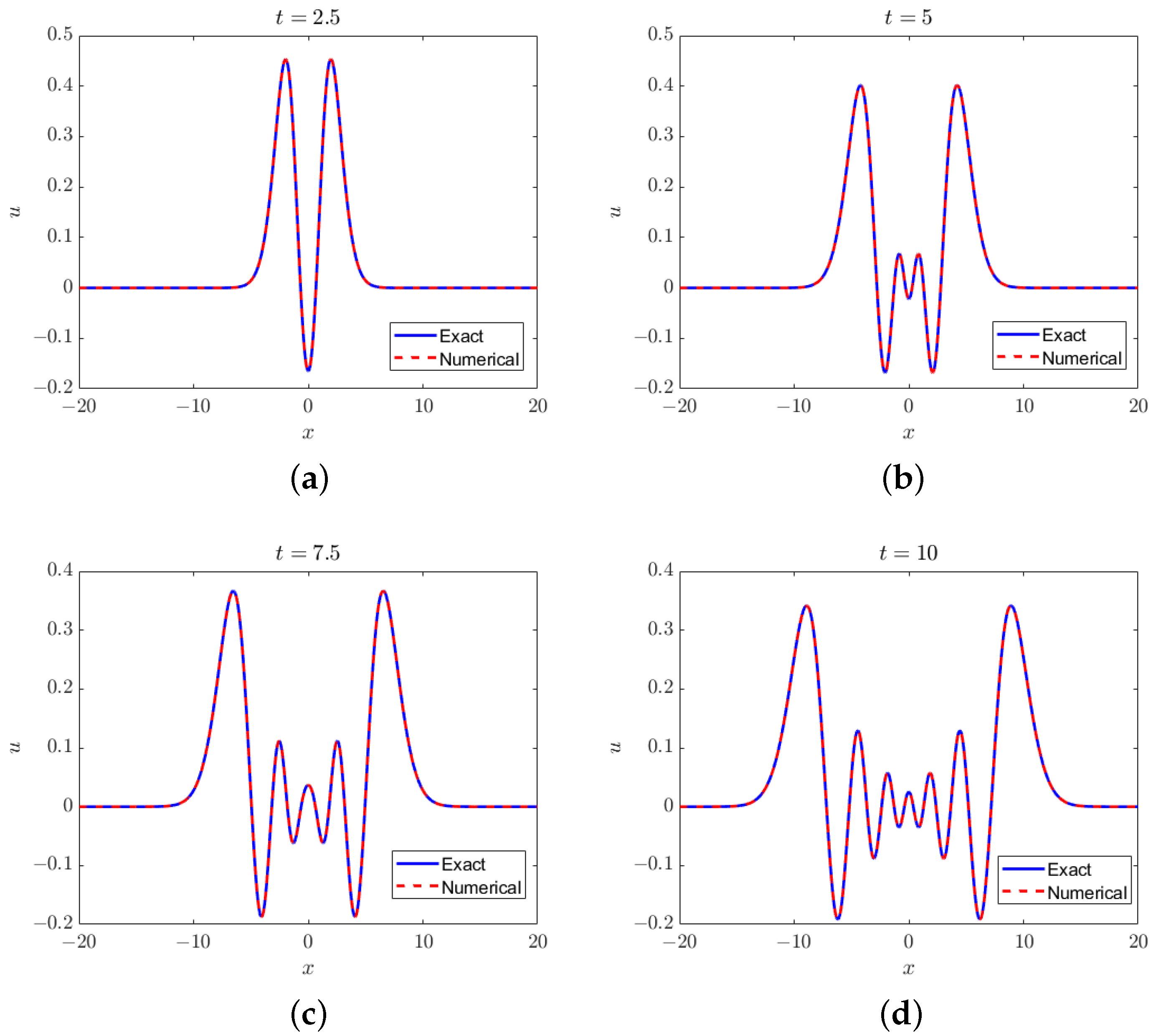
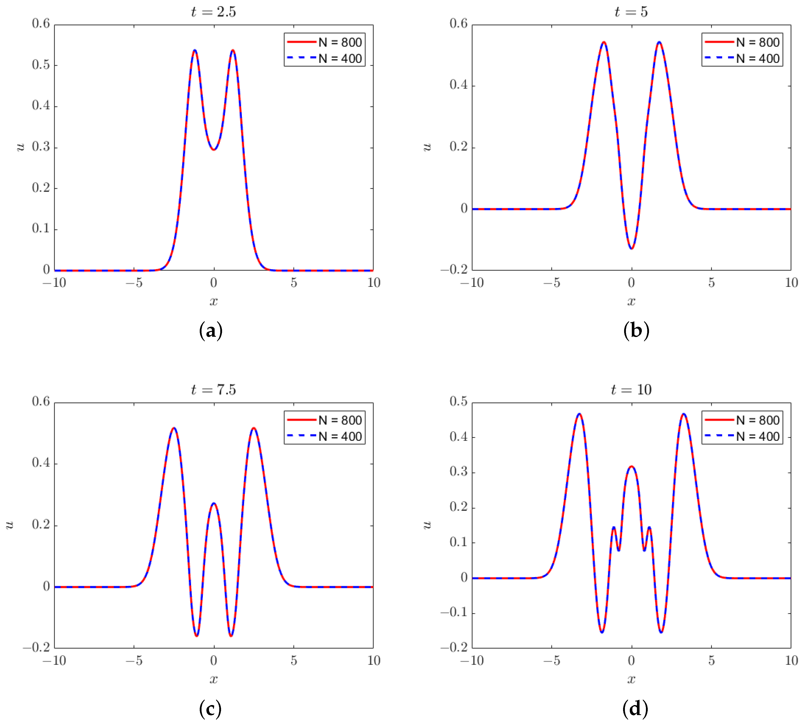
The solutions of the ICN method ($\theta =0.5$) at four time instances are shown in Figure 1. The results are very similar for other values of $\theta$ and the SV method. The grid size is $N=800$. We can see that the numerical solutions agree with the exact solutions very well.

Table 1. Comparison of the SV method and ICN methods with various weights for the linear peridynamic equation. ${ϵ}_{L_2}$ and ${ϵ}_{L_{\infty }}$ represent the numerical errors measured in the $L_2$ and $L_{\infty }$ norms, respectively. $|E_n-E_0|$ denotes the energy variation from $t=0$ to $t=10$.

Method	N	${\mathit{ϵ}}_{{\mathit{L}}_2}$	Rate	${\mathit{ϵ}}_{{\mathit{L}}_{\mathit{\infty }}}$	Rate	$|{\mathit{E}}_{\mathit{n}}-{\mathit{E}}_0|$	Rate
SV	100	1.36 × ${10}^{-3}$	-	3.65 × ${10}^{-2}$	-	3.67 × ${10}^{-2}$	-
	200	2.34 × ${10}^{-4}$	2.54	8.84 × ${10}^{-3}$	2.05	1.83 × ${10}^{-2}$	1.00
	400	4.10 × ${10}^{-5}$	2.51	2.19 × ${10}^{-3}$	2.01	9.18 × ${10}^{-3}$	1.00
	800	7.24 × ${10}^{-6}$	2.50	5.47 × ${10}^{-4}$	2.00	4.59 × ${10}^{-3}$	1.00
	1600	1.28 × ${10}^{-6}$	2.50	1.37 × ${10}^{-4}$	2.00	2.30 × ${10}^{-3}$	1.00
ICN ($\theta =0.5$)	100	2.34 × ${10}^{-3}$	-	6.18 × ${10}^{-2}$	-	3.87 × ${10}^{-1}$	-
	200	4.67 × ${10}^{-4}$	2.32	1.76 × ${10}^{-2}$	1.81	1.45 × ${10}^{-1}$	1.42
	400	8.27 × ${10}^{-5}$	2.50	4.42 × ${10}^{-3}$	2.00	3.89 × ${10}^{-2}$	1.90
	800	1.45 × ${10}^{-5}$	2.51	1.10 × ${10}^{-3}$	2.01	9.84 × ${10}^{-3}$	1.98
	1600	2.56 × ${10}^{-6}$	2.50	2.74 × ${10}^{-4}$	2.00	2.47 × ${10}^{-3}$	2.00
ICN ($\theta =\frac{1}{3}$)	100	7.59 × ${10}^{-4}$	-	2.11 × ${10}^{-2}$	-	1.60 × ${10}^{-1}$	-
	200	7.30 × ${10}^{-5}$	3.38	2.79 × ${10}^{-3}$	2.92	4.99 × ${10}^{-2}$	1.68
	400	6.57 × ${10}^{-6}$	3.47	3.56 × ${10}^{-4}$	2.97	1.30 × ${10}^{-2}$	1.94
	800	5.83 × ${10}^{-7}$	3.49	4.45 × ${10}^{-5}$	3.00	3.28 × ${10}^{-3}$	1.99
	1600	5.16 × ${10}^{-8}$	3.50	5.57 × ${10}^{-6}$	3.00	8.22 × ${10}^{-4}$	2.00
ICN ($\theta =0.25$)	100	1.45 × ${10}^{-3}$	-	3.91 × ${10}^{-2}$	-	1.58 × ${10}^{-2}$	-
	200	2.38 × ${10}^{-4}$	2.61	8.99 × ${10}^{-3}$	2.12	9.70 × ${10}^{-4}$	4.02
	400	4.12 × ${10}^{-5}$	2.53	2.20 × ${10}^{-3}$	2.03	6.06 × ${10}^{-5}$	4.00
	800	7.25 × ${10}^{-6}$	2.51	5.48 × ${10}^{-4}$	2.00	3.79 × ${10}^{-6}$	4.00
	1600	1.28 × ${10}^{-6}$	2.50	1.37 × ${10}^{-4}$	2.00	2.37 × ${10}^{-7}$	4.00

shows the rates of convergence of the solutions measured in the $L_2$ and $L_{\infty }$ norms, together with the energy variation $|E_n-E_0|$. In terms of $L_2$ and $L_{\infty }$ norms, the SV method converges quadratically, the same as the ICN methods with $\theta =0.5$ and $0.25$. When $\theta =1/3$, the ICN method is third-order.

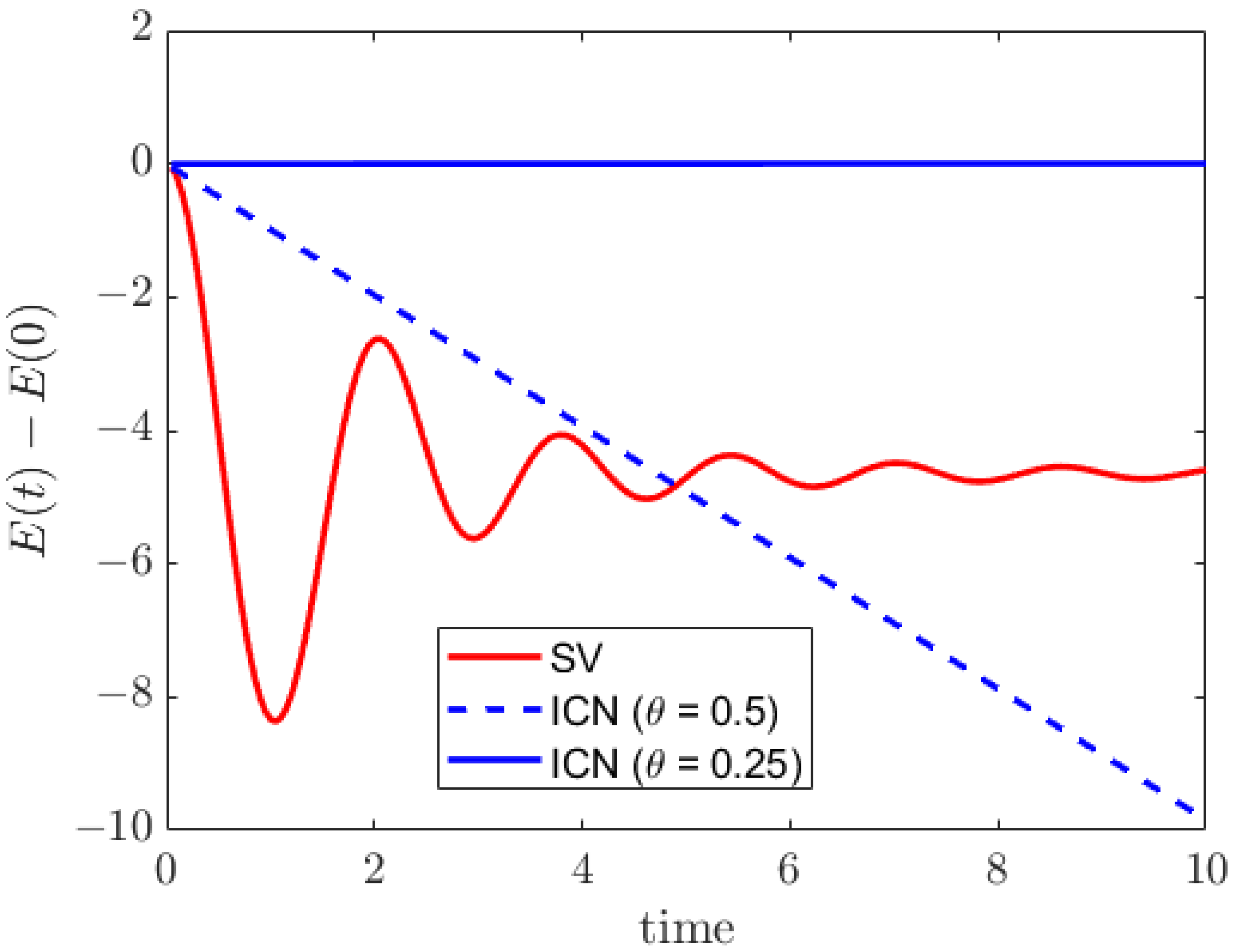
A symplectic method preserves the total energy, meaning the energy variation $|E_n-E_0|=0$ is ideally zero or is on the order of the machine round-off error. However, as shown in Figure 2, the energy variation of the SV method is approximately ${10}^{-3}$, and as illustrated in Table 1, besides being zero, it converges linearly. In the case of the ICN method with $\theta =0.5$, the magnitude of energy variation grows and reaches approximately ${10}^{-2}$ when $t=10$. On the other hand, when $\theta =0.25$, the energy variation grows much more slowly, with its magnitude around ${10}^{-6}$, several orders of magnitude lower than the other two methods. From Table 1, we have the following observations regarding the convergence of the energy variation. Firstly, the ICN method is at least second-order accurate, surpassing the linear convergence of the SV method. Secondly, when $\theta =0.5$, both the energy and the solution exhibit second-order convergence. Thirdly, when $\theta =1/3$, the energy variation converges quadratically, despite its third-order solution. Lastly, when $\theta =0.25$, the ICN method achieves fourth-order superconvergence.

Table 2. Comparison of energy variation and run time for three methods (SV, ICN, and RK4).

Method	$|{\mathit{E}}_{\mathit{n}}-{\mathit{E}}_0|$ ($\mathit{N}=1600$)	Run Time (s)	$|{\mathit{E}}_{\mathit{n}}-{\mathit{E}}_0|$ ($\mathit{N}=3200$)	Run Time (s)
SV	2.30 × ${10}^{-3}$	20	1.15 × ${10}^{-3}$	139
RK4	2.10 × ${10}^{-7}$	33	1.32 × ${10}^{-8}$	236
ICN ($\theta =0.25$)	2.37 × ${10}^{-7}$	26	1.48 × ${10}^{-8}$	184

compares the SV, the ICN with $\theta =0.25$, and the classical RK4 methods. For RK4, both the solution and the energy variation have fourth-order convergence, making it one of the optimal choices for temporal discretization. The energy variation of the SV method is four or five orders of magnitude larger than the other two methods. The ICN method operates approximately 30% slower than the SV method due to the additional evaluation of integrals in the updating equations. The ICN and RK4 methods yield similar energy variation for both resolutions $N=1600$ and $N=3200$, while the ICN solver runs approximately 20% faster than the RK4 method at both resolutions.

4.2. Energy Conservation for the ICN Method with Different Weights

In this test, we investigate the relationship between the energy variation and the weight $\theta$ in the ICN method. The simulation setup remains consistent with the previous section, where the grid size is fixed at $N=800$. The results presented in

Table 3. Energy variation of the ICN method with different weights.

$\mathit{\theta }$	${\mathit{E}}_{\mathit{n}}-{\mathit{E}}_0$
0.70	−1.77 × ${10}^{-2}$
0.60	−1.38 × ${10}^{-2}$
0.50	−9.84 × ${10}^{-3}$
0.40	−5.91 × ${10}^{-3}$
1/3	−3.28 × ${10}^{-3}$
0.30	−1.97 × ${10}^{-3}$
0.25	3.79 × ${10}^{-6}$
0.20	1.98× ${10}^{-3}$

demonstrate that as the weight $\theta$ decreases from 0.7 to 0.2, the energy variation $E_n-E_0$ increases from $-1.7\times {10}^{-2}$ to $1.9\times {10}^{-3}$. Notably, when $\theta =0.25$, the energy variation reaches its minimum amplitude of $3.7\times {10}^{-6}$.

4.3. The ICN Method with Multiple Iterations

In this example, we study the original ICN method ($\theta =0.5$) with a varying number of iterations. Firstly, we examine the relationship between the energy variation and the number of iterations in the ICN method. The simulation setup remains consistent with Section 4.1. We consider two grid sizes: $N=800$ and 1600. As shown in

Table 4. Energy variation of the ICN method when the number of iterations changes. $E_n$ is the total energy at $t=10$.

Number of Iterations m	${\mathit{E}}_{\mathit{n}}-{\mathit{E}}_0$ ($\mathit{N}=800$)	Run Time (s)	${\mathit{E}}_{\mathit{n}}-{\mathit{E}}_0$ ($\mathit{N}=1600$)	Run Time (s)
1	9.88 × ${10}^{-3}$	2.65	2.47 × ${10}^{-3}$	20.44
2	−9.84 × ${10}^{-3}$	3.56	−2.47 × ${10}^{-3}$	29.37
3	−1.51 × ${10}^{-5}$	4.37	−9.47 × ${10}^{-7}$	37.64
4	1.51 × ${10}^{-5}$	5.23	9.47 × ${10}^{-7}$	44.99
5	2.54 × ${10}^{-8}$	6.07	3.98 × ${10}^{-10}$	52.17
6	−2.54 × ${10}^{-8}$	6.92	−3.98 × ${10}^{-10}$	58.95
7	−4.55 × ${10}^{-11}$	7.72	−1.78 × ${10}^{-13}$	66.40
8	4.55 × ${10}^{-11}$	8.58	1.78 × ${10}^{-13}$	72.49
9	8.53 × ${10}^{-14}$	9.45	∼${10}^{-15}$	80.32
10	−8.70 × ${10}^{-14}$	10.27	∼${10}^{-15}$	89.71
11	∼${10}^{-15}$	11.15	∼${10}^{-15}$	95.04
12	∼${10}^{-15}$	11.97	∼${10}^{-15}$	101.81

, as m increases, the energy variation decreases. For $N=800$ and $N=1600$, the energy variations reach the order of the machine round-off error of ${10}^{-15}$ when m is greater than 10 and 8, respectively. This example illustrates that the ICN method can preserve energy up to machine precision by employing a large number of iterations. Furthermore, when the grid size increases, the energy variation reaches machine precision at a faster rate. For $N=1600$, achieving the order of ${10}^{-7}$ requires 3 iterations, with a CPU run time of approximately 37 s. This runtime is not substantially greater than that required for the ICN method with $\theta =0.25$ (26 s) and the RK4 method (33 s) in the previous test, as shown in Table 2.

From the previous multi-iteration test, we observe that when the number of iterations is three, the original ICN method exhibits an energy variation at the same order of magnitude as the RK4 method. This motivates us to conduct a convergence test for the three-iteration ICN method. The results are presented in

Table 5. The three-iteration ICN method ($\theta =0.5$) for linear peridynamic equation.

N	${\mathit{L}}_2$	Rate	${\mathit{L}}_{\mathit{\infty }}$	Rate	|${\mathit{E}}_{\mathit{n}}-{\mathit{E}}_0$|	Rate
100	3.11 × ${10}^{-3}$	-	7.78 × ${10}^{-2}$	-	−5.22 × ${10}^{-2}$	-
200	4.90 × ${10}^{-4}$	2.66	1.86 × ${10}^{-2}$	2.06	−3.77 × ${10}^{-3}$	3.79
400	8.31 × ${10}^{-5}$	2.56	4.44 × ${10}^{-3}$	2.07	−2.41 × ${10}^{-4}$	3.97
800	1.45 × ${10}^{-5}$	2.52	1.10 × ${10}^{-3}$	2.02	−1.51 × ${10}^{-5}$	3.99
1600	2.56 × ${10}^{-6}$	2.50	2.74 × ${10}^{-4}$	2.00	−9.47 × ${10}^{-7}$	4.00

. We find that the three-iteration ICN method demonstrates second-order convergence in terms of the $L_2$ and $L_{\infty }$ error norms, and fourth-order convergence in terms of energy conservation. Since both the three-iteration ICN and the RK4 methods are four-stage methods, they have comparable CPU run times.

Furthermore, we conduct a series of simulations to examine the rate of convergence of the ICN method with varying numbers of iterations, as shown in

Table 6. Energy convergence rate as a function of the number of iterations in the ICN method.

Number of Iterations m	Rate of Convergence of Energy
1	2.0
2	2.0
3	4.0
4	4.0
5	6.0
6	6.0
7	8.0
8	8.0

. We observe that as the number of iterations increases, the rate of convergence also increases. When the number of iterations is an even number, the rate of convergence remains the same as the number of iterations. However, for an odd number of iterations m, the rate of convergence is $m+1$. These results indicate that a higher order of convergence (in terms of energy conservation) can be achieved by increasing the number of iterations in the ICN method.

4.4. Comparison of Three Quadrature Formulas for Linear Peridynamics

As shown in [17], the choice of quadrature formula for integration impacts the accuracy of energy conservation. In this example, we examine three different Newton–Cotes quadrature formulas: the midpoint rule (Equation (19)), the composite trapezoidal rule (Equation (20)), and the composite Simpson’s rule (Equation (21)). For Simpson’s rule, we adjust the grid size to $N+1$, as N is an even number in our simulations. Results are presented in

Table 7. Comparison of three quadrature formulas for the peridynamic simulation using the SV method. ${ϵ}_{L_2}$ and ${ϵ}_{L_{\infty }}$ represent the numerical errors measured in the $L_2$ and $L_{\infty }$ norms, respectively. $|E_n-E_0|$ denotes the energy variation from $t=0$ to $t=10$.

Method	N	${\mathit{ϵ}}_{{\mathit{L}}_2}$	Rate	${\mathit{ϵ}}_{{\mathit{L}}_{\mathit{\infty }}}$	Rate	$|{\mathit{E}}_{\mathit{n}}-{\mathit{E}}_0|$	Rate
SV + midpoint	100	1.3626781938 × ${10}^{-3}$	-	3.6546374629 × ${10}^{-2}$	-	−3.6686416132 × ${10}^{-2}$	-
	200	2.3386240754 × ${10}^{-4}$	2.54	8.8420752239 × ${10}^{-3}$	2.05	−1.8341493309 × ${10}^{-2}$	1.00
	400	4.1038150512 × ${10}^{-5}$	2.51	2.1896453314 × ${10}^{-3}$	2.01	−9.1848205222 × ${10}^{-3}$	1.00
	800	7.2412556153 × ${10}^{-6}$	2.50	5.4733686142 × ${10}^{-4}$	2.00	−4.5945520876 × ${10}^{-3}$	1.00
	1600	1.2794967586 × ${10}^{-6}$	2.50	1.3681318781 × ${10}^{-4}$	2.00	−2.2975549644 × ${10}^{-3}$	1.00
SV + composite trapezoidal	100	1.3626781938 × ${10}^{-3}$	-	3.6546374631 × ${10}^{-2}$	-	−3.6686416132 × ${10}^{-2}$	-
	200	2.3386240741 × ${10}^{-4}$	2.54	8.8420752309 × ${10}^{-3}$	2.05	−1.8341493309 × ${10}^{-2}$	1.00
	400	4.1038150469 × ${10}^{-5}$	2.51	2.1896453350 × ${10}^{-3}$	2.01	−9.1848205222 × ${10}^{-3}$	1.00
	800	7.2412556001 × ${10}^{-6}$	2.50	5.4733686322 × ${10}^{-4}$	2.00	−4.5945520876 × ${10}^{-3}$	1.00
	1600	1.2794967533 × ${10}^{-6}$	2.50	1.3681318870 × ${10}^{-4}$	2.00	−2.2975549644 × ${10}^{-3}$	1.00
SV + composite Simpson	100	1.3532560898 × ${10}^{-3}$	-	3.6461913740 × ${10}^{-2}$	-	−3.6637130961 × ${10}^{-2}$	-
	200	2.3386240745 × ${10}^{-4}$	2.53	8.8420752291 × ${10}^{-3}$	2.04	−1.8341493309 × ${10}^{-2}$	1.00
	400	4.1038150476 × ${10}^{-5}$	2.51	2.1896453345 × ${10}^{-3}$	2.01	−9.1848205222 × ${10}^{-3}$	1.00
	800	7.2412556013 × ${10}^{-6}$	2.50	5.4733686308 × ${10}^{-4}$	2.00	−4.5945520876 × ${10}^{-3}$	1.00
	1600	1.2794967535 × ${10}^{-6}$	2.50	1.3681318867 × ${10}^{-4}$	2.00	−2.2975549644 × ${10}^{-3}$	1.00

and

Table 8. Comparison of three quadrature formulas for the peridynamic simulation using the ICN method ($\theta =0.25$). ${ϵ}_{L_2}$ and ${ϵ}_{L_{\infty }}$ represent the numerical errors measured in the $L_2$ and $L_{\infty }$ norms, respectively. $|E_n-E_0|$ denotes the energy variation from $t=0$ to $t=10$.

Method	N	${\mathit{ϵ}}_{{\mathit{L}}_2}$	Rate	${\mathit{ϵ}}_{{\mathit{L}}_{\mathit{\infty }}}$	Rate	$|{\mathit{E}}_{\mathit{n}}-{\mathit{E}}_0|$	Rate
ICN + midpoint	100	1.4531942146 × ${10}^{-3}$	-	3.9071358030 × ${10}^{-2}$	-	1.5796799025 × ${10}^{-2}$	-
	200	2.3797519266 × ${10}^{-4}$	2.61	8.9850019534 × ${10}^{-3}$	2.12	9.7041252646 × ${10}^{-4}$	4.02
	400	4.1222863495 × ${10}^{-5}$	2.53	2.1984031675 × ${10}^{-3}$	2.03	6.0617629614 × ${10}^{-5}$	4.00
	800	7.2494508340 × ${10}^{-6}$	2.51	5.4789636190 × ${10}^{-4}$	2.00	3.7885364605 × ${10}^{-6}$	4.00
	1600	1.2798591070 × ${10}^{-6}$	2.50	1.3684841395 × ${10}^{-4}$	2.00	2.3678339289 × ${10}^{-7}$	4.00
ICN + composite trapezoidal	100	1.4531942145 × ${10}^{-3}$	-	3.9071358029 × ${10}^{-2}$	-	1.5796799025 × ${10}^{-2}$	-
	200	2.3797519254 × ${10}^{-4}$	2.61	8.9850019605 × ${10}^{-3}$	2.12	9.7041252645 × ${10}^{-4}$	4.02
	400	4.1222863452 × ${10}^{-5}$	2.53	2.1984031712 × ${10}^{-3}$	2.03	6.0617629611 × ${10}^{-5}$	4.00
	800	7.2494508188 × ${10}^{-6}$	2.51	5.4789636369 × ${10}^{-4}$	2.00	3.7885364605 × ${10}^{-6}$	4.00
	1600	1.2798591017 × ${10}^{-6}$	2.50	1.3684841484 × ${10}^{-4}$	2.00	2.3678340710 × ${10}^{-7}$	4.00
ICN + composite Simpson	100	1.4433953589 × ${10}^{-3}$	-	3.8867087321 × ${10}^{-2}$	-	1.5770288980 × ${10}^{-2}$	-
	200	2.3797519257 × ${10}^{-4}$	2.60	8.9850019587 × ${10}^{-3}$	2.11	9.7041252645 × ${10}^{-4}$	4.02
	400	4.1222863459 × ${10}^{-5}$	2.53	2.1984031706 × ${10}^{-3}$	2.03	6.0617629612 × ${10}^{-5}$	4.00
	800	7.2494508201 × ${10}^{-6}$	2.51	5.4789636355 × ${10}^{-4}$	2.00	3.7885364570 × ${10}^{-6}$	4.00
	1600	1.2798591019 × ${10}^{-6}$	2.50	1.3684841481 × ${10}^{-4}$	2.00	2.3678339645 × ${10}^{-7}$	4.00

. We do not observe significant differences among the three quadrature formulas. All three methods exhibit the same order of convergence. The $L_2$, $L_{\infty }$, and energy variation are of comparable magnitudes across all three methods, with the differences being negligible. This example suggests that the degree of the Newton–Cotes quadrature formulas does not significantly affect the convergence rate.

4.5. Linear Peridynamic Model with Discontinuous Initial Condition

In this example, we explore our method’s capability for handling discontinuities, focusing on discontinuous initial conditions [34,35]. The simulation setup mirrors the previous linear example in Section 4.1, except for the initial condition.

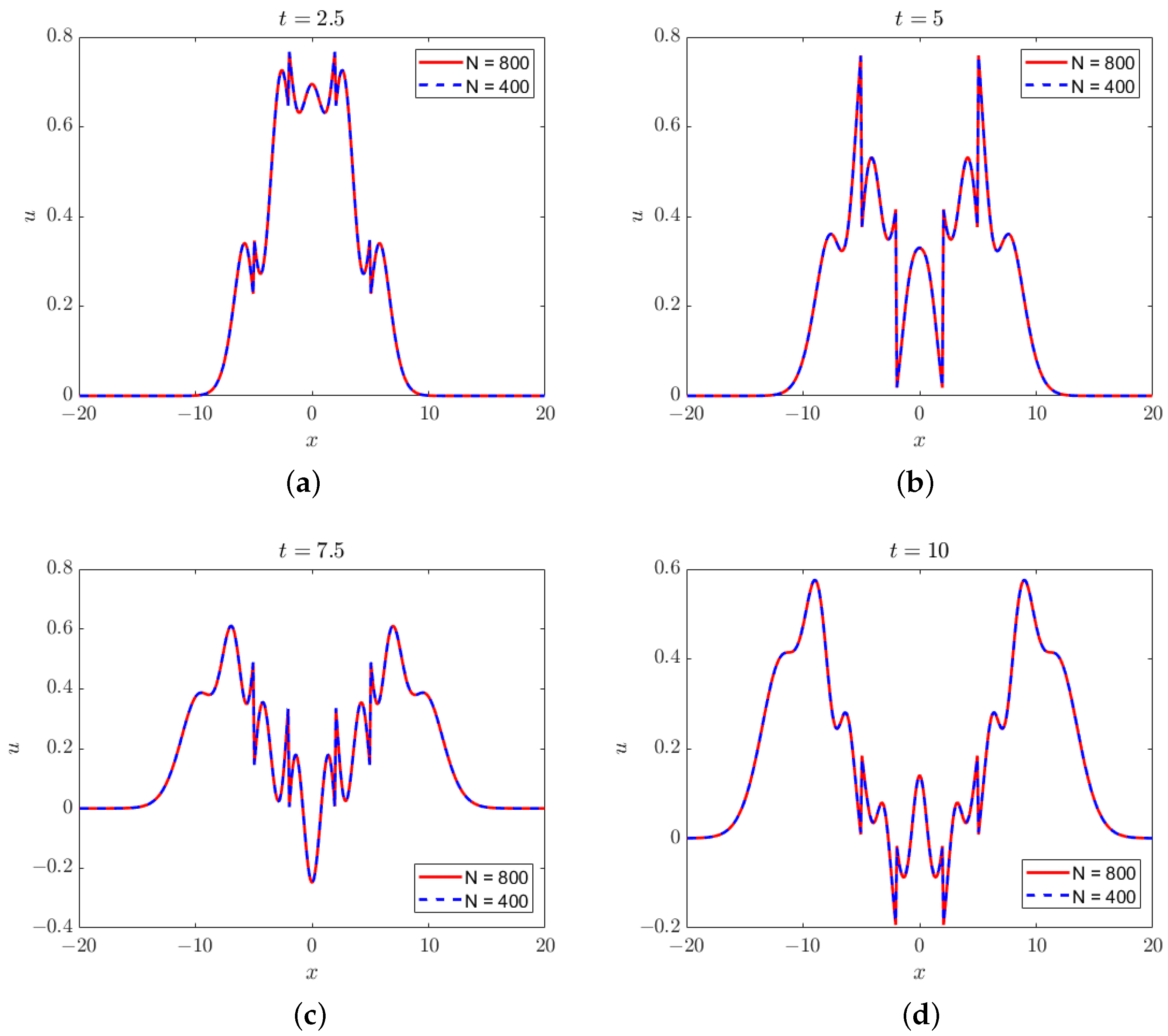
First, we utilize the following piecewise constant function as the initial displacement field $u_0$:

$$u_0\left(x\right)=\left\{\begin{array}{cc}1,& \left|x\right|<2\\ 0.5,& 2\le \left|x\right|<5\\ 0,& \mathrm{otherwise}.\end{array}\right.$$

(48)

The initial velocity field $v_0$ is set to zero. The solutions of the ICN method ($\theta =0.25$) at four time instances are shown in Figure 3, and the convergence rates are listed in

Table 9. Numerical errors and convergence rates of the SV and the ICN methods for the linear peridynamic equation with piecewise constant initial displacement field (48). ${ϵ}_{L_2}$ and ${ϵ}_{L_{\infty }}$ represent the numerical errors measured in the $L_2$ and $L_{\infty }$ norms, respectively. $|E_n-E_0|$ denotes the energy variation from $t=0$ to $t=10$.

Method	N	${\mathit{ϵ}}_{{\mathit{L}}_2}$	Rate	${\mathit{ϵ}}_{{\mathit{L}}_{\mathit{\infty }}}$	Rate	$|{\mathit{E}}_{\mathit{n}}-{\mathit{E}}_0|$	Rate
SV	100	3.31 × ${10}^{-3}$	-	1.03 × ${10}^{-1}$	-	6.40 × ${10}^{-2}$	-
	200	4.78 × ${10}^{-4}$	2.79	2.74 × ${10}^{-2}$	1.91	3.26 × ${10}^{-2}$	0.97
	400	8.17 × ${10}^{-5}$	2.55	7.53 × ${10}^{-3}$	1.86	1.63 × ${10}^{-2}$	1.00
	800	1.36 × ${10}^{-5}$	2.58	1.90 × ${10}^{-3}$	1.99	8.14 × ${10}^{-3}$	1.00
	1600	1.89 × ${10}^{-6}$	2.85	3.91 × ${10}^{-4}$	2.28	4.06 × ${10}^{-3}$	1.00
ICN ($\theta =0.25$)	100	3.53 × ${10}^{-3}$	-	1.09 × ${10}^{-1}$	-	3.13 × ${10}^{-2}$	-
	200	4.89 × ${10}^{-4}$	2.85	2.81 × ${10}^{-2}$	1.95	2.00 × ${10}^{-3}$	3.96
	400	8.22 × ${10}^{-5}$	2.57	7.59 × ${10}^{-3}$	1.89	1.26 × ${10}^{-4}$	3.99
	800	1.37 × ${10}^{-5}$	2.59	1.90 × ${10}^{-3}$	2.00	7.88 × ${10}^{-6}$	4.00
	1600	1.89 × ${10}^{-6}$	2.85	3.91 × ${10}^{-4}$	2.28	4.92 × ${10}^{-7}$	4.00

.

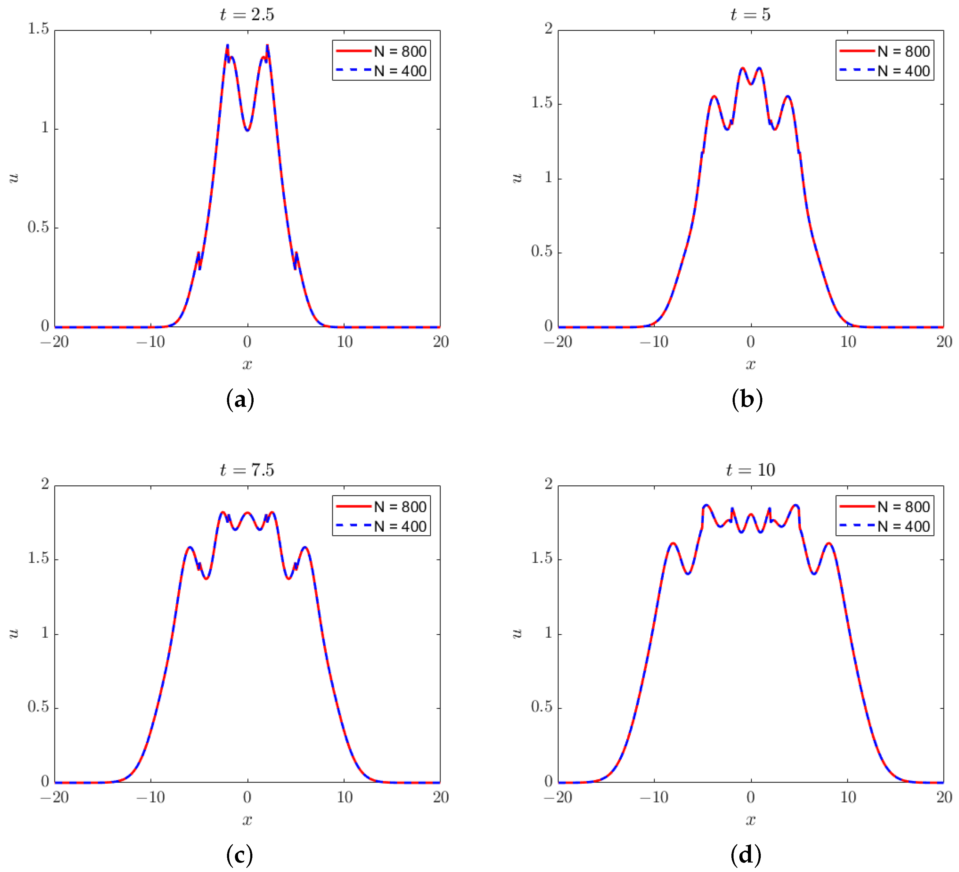
For the second experiment in this section, we apply a piecewise constant function as the initial velocity field $v_0$:

$$v_0\left(x\right)=\left\{\begin{array}{cc}0.5,& \left|x\right|<2\\ 0.25,& 2\le \left|x\right|<5\\ 0,& \mathrm{otherwise}.\end{array}\right.$$

(49)

The initial displacement field is a continuous function $u_0\left(x\right)=exp(-x^2)$. The results are presented in Figure 4 and in

Table 10. Numerical errors and convergence rates of the SV and the ICN methods for the linear peridynamic equation with piecewise constant initial velocity field (49). ${ϵ}_{L_2}$ and ${ϵ}_{L_{\infty }}$ represent the numerical errors measured in the $L_2$ and $L_{\infty }$ norms, respectively. $|E_n-E_0|$ denotes the energy variation from $t=0$ to $t=10$.

Method	N	${\mathit{ϵ}}_{{\mathit{L}}_2}$	Rate	${\mathit{ϵ}}_{{\mathit{L}}_{\mathit{\infty }}}$	Rate	$|{\mathit{E}}_{\mathit{n}}-{\mathit{E}}_0|$	Rate
SV	100	3.47 × ${10}^{-3}$	-	8.95 × ${10}^{-2}$	-	2.99 × ${10}^{-2}$	-
	200	2.69 × ${10}^{-4}$	3.69	9.93 × ${10}^{-3}$	3.17	1.51 × ${10}^{-2}$	0.99
	400	4.69 × ${10}^{-5}$	2.52	2.61 × ${10}^{-3}$	1.93	7.54 × ${10}^{-3}$	1.00
	800	7.93 × ${10}^{-6}$	2.56	6.62 × ${10}^{-4}$	1.98	3.76 × ${10}^{-3}$	1.00
	1600	1.15 × ${10}^{-6}$	2.78	1.41 × ${10}^{-4}$	2.23	1.88 × ${10}^{-3}$	1.00
ICN ($\theta =0.25$)	100	3.50 × ${10}^{-3}$	-	9.14 × ${10}^{-2}$	-	1.04 × ${10}^{-2}$	-
	200	2.64 × ${10}^{-4}$	3.73	9.78 × ${10}^{-3}$	3.22	6.35 × ${10}^{-4}$	4.03
	400	4.55 × ${10}^{-5}$	2.54	2.38 × ${10}^{-3}$	2.04	3.94 × ${10}^{-5}$	4.01
	800	7.67 × ${10}^{-6}$	2.57	5.81 × ${10}^{-4}$	2.04	2.45 × ${10}^{-6}$	4.01
	1600	1.11 × ${10}^{-6}$	2.78	1.25 × ${10}^{-4}$	2.22	1.53 × ${10}^{-7}$	4.00

. When computing the convergence rates, we utilize the solution obtained on a fine mesh ($N=3200$) as the reference solution. In both scenarios, the convergence rates are akin to those observed with continuous initial conditions. Specifically, with regard to the $L_2$ and $L_{\infty }$ error norms, both the SV method and the ICN method demonstrate quadratic convergence. In terms of energy conservation, the SV method displays linear convergence, whereas the ICN method with $\theta =0.25$ achieves fourth-order accuracy.

4.6. Nonlinear Peridynamic Equation

For the nonlinear case, we set $r=3$ in Equation (43). The computational domain spans $[-10,10]$, with $\Delta t=\Delta x$. The solution obtained through the ICN method is presented in Figure 5, and

Table 11. Comparison of the SV method and the ICN methods with various weights for the nonlinear peridynamic equation. ${ϵ}_{L_2}$ and ${ϵ}_{L_{\infty }}$ represent the numerical errors measured in the $L_2$ and $L_{\infty }$ norms, respectively.

Method	N	${\mathit{ϵ}}_{{\mathit{L}}_2}$	Rate	${\mathit{ϵ}}_{{\mathit{L}}_{\mathit{\infty }}}$	Rate
SV	100	2.12 × ${10}^{-4}$	-	4.45 × ${10}^{-3}$	-
	200	2.33 × ${10}^{-5}$	3.19	7.04 × ${10}^{-4}$	2.66
	400	4.11 × ${10}^{-6}$	2.50	1.91 × ${10}^{-4}$	1.88
	800	7.65 × ${10}^{-7}$	2.42	6.45 × ${10}^{-5}$	1.57
ICN ($\theta =0.5$)	100	2.15 × ${10}^{-4}$	-	7.65 × ${10}^{-2}$	-
	200	2.46 × ${10}^{-5}$	3.13	1.54 × ${10}^{-2}$	2.31
	400	4.20 × ${10}^{-6}$	2.55	3.01 × ${10}^{-3}$	2.36
	800	7.68 × ${10}^{-7}$	2.45	6.26 × ${10}^{-4}$	2.27
ICN ($\theta =\frac{1}{3}$)	100	8.39 × ${10}^{-4}$	-	2.14 × ${10}^{-2}$	-
	200	8.03 × ${10}^{-5}$	3.39	2.84 × ${10}^{-3}$	2.92
	400	7.36 × ${10}^{-6}$	3.45	3.63 × ${10}^{-4}$	2.97
	800	6.59 × ${10}^{-7}$	3.48	5.17 × ${10}^{-5}$	2.81
ICN ($\theta =0.25$)	100	3.11 × ${10}^{-4}$	-	8.13 × ${10}^{-3}$	-
	200	3.34 × ${10}^{-5}$	3.22	1.16 × ${10}^{-3}$	2.81
	400	4.77 × ${10}^{-6}$	2.81	2.40 × ${10}^{-4}$	2.27
	800	7.92 × ${10}^{-7}$	2.59	7.16 × ${10}^{-5}$	1.75

illustrates the convergence rates of these solutions. We use the solution on a fine mesh ($N=3200$) as the exact solution when computing the convergence rates. From the tabulated data, it is evident that when $\theta =1/3$, the ICN method demonstrates third-order convergence. For the other two values of $\theta$, the ICN method converges quadratically, similar to the SV method.

5. Conclusions

In summary, we utilized the iterated Crank–Nicolson (ICN) algorithms to solve the integro-differential equation for peridynamic models. The weighted ICN method, a generalization of the original ICN method that introduces a weight $\theta$ while maintaining at least second-order accuracy, was employed for temporal discretization. Additionally, we employed a midpoint quadrature algorithm for numerical integration in the spatial domain.

A series of numerical simulations were conducted to assess the performance of the ICN method for linear and nonlinear peridynamic equations in one dimension. The results confirmed the convergence rates of the ICN methods with various weights, including $\theta =0.5$, $1/3$, and $0.25$. Additionally, we compared three quadrature formulas and observed similar results for both the Störmer–Verlet (SV) and ICN methods, indicating that the choice of quadrature formula does not significantly affect the rate of convergence.

Our focus on energy conservation in the linear peridynamic model led to several key observations. Firstly, for the original ICN method with $\theta =0.5$, increasing the number of iterations reduced the energy variation until it reached machine precision, with the convergence rate increasing as iterations increased. Secondly, decreasing $\theta$ resulted in a corresponding decrease in the magnitude of the energy variation, with $\theta =0.25$ yielding the minimum value. Thirdly, we noted that the rate of energy convergence was lower than that of the solution for the SV method and the ICN method with $\theta =1/3$. While the SV method exhibited second-order convergence with linear energy convergence, the ICN method with $\theta =1/3$ achieved third-order accuracy with quadratic energy convergence. When $\theta =0.5$, both the solution and the energy variation were second-order convergent. Finally, when $\theta =0.25$, the ICN method demonstrated fourth-order superconvergence regarding energy conservation, with energy variation at the same order of magnitude as the fourth-order Runge–Kutta method while saving approximately 20% of the CPU time. Similar results were obtained with piecewise constant initial conditions, and a nonlinear case was also tested to verify the rate of convergence of the ICN method.

In conclusion, our numerical tests demonstrated that the ICN method is well suited for peridynamic simulation and generally outperforms the SV method in terms of energy conservation.

References

- Silling, S.A. Reformulation of elasticity theory for discontinuities and long-range forces. J. Mech. Phys. Solids 2000, 48, 175–209. [Google Scholar] [CrossRef]
- Silling, S.A.; Lehoucq, R.B. Peridynamic theory of solid mechanics. Adv. Appl. Mech. 2010, 44, 73–168. [Google Scholar]
- Madenci, E.; Oterkus, E. Peridynamic Theory and Its Applications; Springer: New York, NY, USA, 2014. [Google Scholar]
- Bobaru, F.; Foster, J.T.; Geubelle, P.H.; Silling, S.A. Handbook of Peridynamic Modeling; CRC Press: Boca Raton, FL, USA, 2016. [Google Scholar]
- Javili, A.; Morasata, R.; Oterkus, E.; Oterkus, S. Peridynamics review. Math. Mech. Solids 2019, 24, 3714–3739. [Google Scholar] [CrossRef]
- Silling, S.A.; Askari, E. A meshfree method based on the peridynamic model of solid mechanics. Comput. Struct. 2005, 83, 1526–1535. [Google Scholar] [CrossRef]
- Weckner, O.; Emmrich, E. Numerical simulation of the dynamics of a nonlocal, inhomogeneous, infinite bar. J. Comput. Appl. Mech. 2005, 6, 311–319. [Google Scholar]
- Emmrich, E.; Weckner, O. The peridynamic equation and its spatial discretisation. Math. Model. Anal. 2007, 12, 17–27. [Google Scholar] [CrossRef]
- Macek, R.W.; Silling, S.A. Peridynamics via finite element analysis. Finite Elem. Anal. Des. 2007, 43, 1169–1178. [Google Scholar] [CrossRef]
- Tian, X.; Du, Q. Nonconforming discontinuous Galerkin methods for nonlocal variational problems. SIAM J. Numer. Anal. 2015, 53, 762–781. [Google Scholar] [CrossRef]
- Lopez, L.; Pellegrino, S.F. A spectral method with volume penalization for a nonlinear peridynamic model. Int. J. Numer. Methods Eng. 2021, 122, 707–725. [Google Scholar] [CrossRef]
- Lopez, L.; Pellegrino, S.F. A nonperiodic Chebyshev spectral method avoiding penalization techniques for a class of nonlinear peridynamic models. Int. J. Numer. Methods Eng. 2022, 123, 4859–4876. [Google Scholar] [CrossRef]
- Lopez, L.; Pellegrino, S.F. A space-time discretization of a nonlinear peridynamic model on a 2D lamina. Comput. Math. Appl. 2022, 116, 161–175. [Google Scholar] [CrossRef]
- Lopez, L.; Pellegrino, S.F. A fast-convolution based space–time Chebyshev spectral method for peridynamic models. Adv. Contin. Discret. Model. 2022, 2022, 70. [Google Scholar] [CrossRef]
- Hairer, E.; Lubich, C.; Wanner, G. Geometric numerical integration illustrated by the Störmer–Verlet method. Acta Numer. 2003, 12, 399–450. [Google Scholar] [CrossRef]
- Seleson, P.; Pasetto, M.; John, Y.; Trageser, J.; Reeve, S.T. PDMATLAB2D: A Peridynamics MATLAB Two-dimensional Code. J. Peridyn. Nonlocal Model. 2024, 1–57. [Google Scholar] [CrossRef]
- Coclite, G.M.; Fanizzi, A.; Lopez, L.; Maddalena, F.; Pellegrino, S.F. Numerical methods for the nonlocal wave equation of the peridynamics. Appl. Numer. Math. 2020, 155, 119–139. [Google Scholar] [CrossRef]
- Crank, J.; Nicolson, P. A practical method for numerical evaluation of solutions of partial differential equations of the heat-conduction type. In Mathematical Proceedings of the Cambridge Philosophical Society; Cambridge University Press: Cambridge, UK, 1947; Volume 43, pp. 50–67. [Google Scholar]
- Choptuik, M.W. Critical behaviour in scalar field collapse. In Deterministic Chaos in General Relativity; Springer: Boston, MA, USA, 1994; pp. 155–175. [Google Scholar]
- Teukolsky, S.A. Stability of the iterated Crank-Nicholson method in numerical relativity. Phys. Rev. D 2000, 61, 087501. [Google Scholar] [CrossRef]
- Duez, M.D.; Marronetti, P.; Shapiro, S.L.; Baumgarte, T.W. Hydrodynamic simulations in 3 + 1 general relativity. Phys. Rev. D 2003, 67, 024004. [Google Scholar] [CrossRef]
- Duez, M.D.; Liu, Y.T.; Shapiro, S.L.; Stephens, B.C. General relativistic hydrodynamics with viscosity: Contraction, catastrophic collapse, and disk formation in hypermassive neutron stars. Phys. Rev. D 2004, 69, 104030. [Google Scholar] [CrossRef]
- Yioultsis, T.V.; Ziogos, G.D.; Kriezis, E.E. Explicit finite-difference vector beam propagation method based on the iterated Crank-Nicolson scheme. JOSA A 2009, 26, 2183–2191. [Google Scholar] [CrossRef] [PubMed]
- Ketzaki, D.A.; Rekanos, I.T.; Kosmanis, T.I.; Yioultsis, T.V. Beam Propagation Method Based on the Iterated Crank–Nicolson Scheme for Solving Large-Scale Wave Propagation Problems. IEEE Trans. Magn. 2015, 51, 7204404. [Google Scholar] [CrossRef]
- Shibayama, J.; Nishio, T.; Yamauchi, J.; Nakano, H. Explicit FDTD method based on iterated Crank–Nicolson scheme. Electron. Lett. 2022, 58, 16–18. [Google Scholar] [CrossRef]
- Wu, P.; Wang, X.; Xie, Y.; Jiang, H.; Natsuki, T. Iterated Crank-Nicolson Procedure with Enhanced Absorption for Nonuniform Domains. IEEE J. Multiscale Multiphysics Comput. Tech. 2022, 7, 61–68. [Google Scholar] [CrossRef]
- Leiler, G.; Rezzolla, L. Iterated Crank-Nicolson method for hyperbolic and parabolic equations in numerical relativity. Phys. Rev. D 2006, 73, 044001. [Google Scholar] [CrossRef]
- Tran, Q.; Liu, J. Modified iterated Crank-Nicolson method with improved accuracy for advection equations. Numer. Algorithms 2023, 1–22. [Google Scholar] [CrossRef]
- Butcher, J.C. Numerical Methods for Ordinary Differential Equations; John Wiley & Sons: Hoboken, NJ, USA, 2016. [Google Scholar]
- Burden, R.L. Numerical Analysis; Brooks/Cole Cengage Learning: Boston, MA, USA, 2011. [Google Scholar]
- Gottlieb, S.; Shu, C.W. Total variation diminishing Runge-Kutta schemes. Math. Comput. 1998, 67, 73–85. [Google Scholar] [CrossRef]
- Gottlieb, S.; Shu, C.W.; Tadmor, E. Strong stability-preserving high-order time discretization methods. SIAM Rev. 2001, 43, 89–112. [Google Scholar] [CrossRef]
- Weckner, O.; Abeyaratne, R. The effect of long-range forces on the dynamics of a bar. J. Mech. Phys. Solids 2005, 53, 705–728. [Google Scholar] [CrossRef]
- Emmrich, E.; Weckner, O. Analysis and numerical approximation of an integro-differential equation modeling non-local effects in linear elasticity. Math. Mech. Solids 2007, 12, 363–384. [Google Scholar] [CrossRef]
- Difonzo, F.V.; Di Lena, F. Numerical Modeling of Peridynamic Richards’ Equation with Piecewise Smooth Initial Conditions Using Spectral Methods. Symmetry 2023, 15, 960. [Google Scholar] [CrossRef]
Figure 1.
Solutions to the linear peridynamic equation at (a) , (b) , (c) , and (d) . Method: the ICN method with . Mesh size .
Figure 2.
Time history of the total energy variation . The grid size is .
Figure 3.
Solutions of the linear peridynamic equation with piecewise constant initial displacement field (
48) at (
a)
, (
b)
c)
, and (
d)
.
Figure 4.
Solutions of the linear peridynamic equation with piecewise constant initial velocity field (
49) at (
Figure 5.
Solutions to the nonlinear peridynamic equation at (a) , (b) , (c) , and (d) .