Porous and Magnetic Effects on Modified Stokes’ Problems for Generalized Burgers’ Fluids

Abstract

In this paper, exact analytical expressions are derived for dimensionless steady-state solutions corresponding to the modified Stokes’ problems for incompressible generalized Burgers’ fluids, considering the influence of porous and magnetic effects. Actually, these are the first exact solutions for such motions of these fluids. They can easily be particularized to give similar solutions for Newtonian, second-grade, Maxwell, Oldroyd-B and Burgers’ fluids. It is also proven that MHD motion problems of such fluids between infinite parallel plates can be investigated when shear stress is applied at the boundary. To validate the obtained results, the velocity fields are presented in two distinct forms, and their equivalence is proven through graphical representations. The obtained outcomes are utilized to determine the time required to reach a steady state and to elucidate the impacts of porous and magnetic parameters on the fluid motion. This investigation reveals that the attainment of a steady state occurs later when a porous medium or magnetic field is present. Additionally, the fluid’s flow resistance is augmented in the presence of a magnetic field or through a porous medium. Thus, as was expected, the fluid moves slower through porous media or in the presence of a magnetic field.

1. Introduction

Incompressible generalized Burgers’ fluids (IGBFs), as they have been defined by Fetecau et al. [1], are characterized by the following constitutive equations:

$$\mathit{T}=-\tilde{p}\mathit{I}+\mathit{S}, \left(1+{\tilde{\lambda }}_1\frac{\delta }{\delta \tau }+{\tilde{\lambda }}_2\frac{{\delta }^2}{\delta {\tau }^2}\right)\mathit{S}=\mu \left(1+{\tilde{\lambda }}_3\frac{\delta }{\delta \tau }+{\tilde{\lambda }}_4\frac{{\delta }^2}{\delta {\tau }^2}\right)\mathit{A} ,$$

(1)

where T, S, A and $-\tilde{p}\mathit{I}$ have well known significations, $\mu$ is the dynamic viscosity, ${\tilde{\lambda }}_i (i=1,2,3,4)$ are material constants and $\delta /\delta \tau$ denotes the upper-convected time derivative. As compared with the incompressible Burgers’ model [2], a novel material parameter represented by ${\tilde{\lambda }}_4$ emerges within the constitutive equations. The first precise solutions for unsteady motions of IGBFs appear to be those proposed by Fetecau et al. [1] within rectangular regions. Additional noteworthy solutions describing different unsteady motions of the same fluids in such a domain have been identified by Zheng et al. [3], Jamil [4], Fetecau et al. [5] and Khan et al. [6]. Starting solutions for oscillatory motions of these fluids have been established by Tong [7] in cylindrical domains.

Recently, different authors have undertaken examinations of the magnetohydrodynamic (MHD) motions of IGBFs fluids when they pass through porous media. The interplay between a magnetic field and a flowing electrically conductive fluid leads to significant effects in the fields of physics, chemistry and engineering. The steady MHD flow of Newtonian fluids between two infinite parallel plates has been relatively recently investigated by Kiema et al. [8] using Sumudu transform. Exact solutions concerning MHD movements of IGBFs have been established by Sultan et al. [9,10] for scenarios where the fluids are situated between parallel walls that are perpendicular to a plate. Concurrently, the flows of fluids through porous media hold diverse applications in areas such as oil reservoir technology, the petroleum industry, as well as geophysical and astrophysical investigations. The first exact solutions for MHD movements of IGBFs through porous media appear to have been formulated by Khan et al. [11] for the second problem of Stokes. Further interesting exact solutions for such fluid motions of these fluids through a porous medium have been developed by Abro et al. [12], Alqahtani and Khan [13] and Hussain et al. [14] using integral transform techniques. In a recent development, Fetecau and Morosanu [15] introduced simplified expressions for dimensionless steady-state solutions pertaining to MHD Stokes’ problems involving IGBFs that traverse through porous media. These solutions rectify certain inaccuracies found in earlier findings within the existing body of literature.

The central objective of this study is to formulate expressions in closed form for dimensionless steady-state solutions pertaining to the modified Stokes’ problems involving IGBFs, while simultaneously accounting for the effects of magnetism and porosity. For the purpose of verification, the velocity fields are presented in distinct forms, and their equivalence is visually demonstrated. Moreover, the convergence of starting solutions to their corresponding steady-state components is provided, along with the determination of the time required for achieving a steady state. Additionally, the obtained solutions can be readily adapted to yield analogous outcomes for other fluid types such as incompressible Burgers, Oldroyd-B, Maxwell, second-grade and Newtonian fluids. In addition, the possibility of finding exact solutions for such MHD motions of rate-type fluids when shear stress is applied at the boundary is brought to light. The impact of the magnetic field and porous medium on the resistance to fluid flow is also explored. The findings indicate that fluid movement experiences a decrease in speed when passing through a porous medium or in the presence of a magnetic field.

2. Governing Equations

Let us assume that an electrically conducting IGBF is at rest in a porous space between two infinite horizontal parallel plates. At the moment $\tau =0^{+}$, the lower plate begins to oscillate in its plane with a velocity of $\tilde{W}\cos (\omega \tau )$ or $\tilde{W}\sin (\omega \tau )$, and a magnetic field of magnitude B acts vertical to plates. The constants $\omega$ and $\tilde{W}$ denote the frequency and the amplitude of the oscillations, respectively. The fluid motion due to sine oscillations of the lower plate has been called “modified Stokes’ second problem” by Rajagopal et al. [16]. We also assume that the fluid, whose magnetic Reynolds number is small enough [17], is finitely conducting. Consequently, the induced magnetic field and the Joule heating can be neglected. Moreover, we suppose there exists no surplus electric charge distribution, and Hall effects can be ignored owing to the moderate values of the magnetic parameter.

Due to the shear, the fluid is gradually moved and the velocity vector corresponding to these motions is given by the relation [1,11]

$$\tilde{\mathit{w}}=\tilde{\mathit{w}}(z,\tau )=\tilde{w}(z,\tau )\mathit{j},$$

(2)

reported to be a suitable Cartesian coordinate system (x, y and z) whose z-axis is vertical to the plates. Here, j is the unit vector along the y-axis. For such motions, the continuity equation is identically satisfied. We also assume that the extra-stress tensor S, as well as the velocity vector $\tilde{\mathit{w}}$, is a function of z and $\tau$ only.

Substituting $\tilde{\mathit{w}}(z,\tau )$ from Equation (2) into the second constitutive Equation (1), and bearing in mind the fact that the fluid has been at rest up to the initial moment $\tau =0$, it results that the components $S_{xx}, S_{zz}, S_{zx}$ and $S_{xy}$ of the extra-stress tensor S are zero. In addition, the tangential shear stress $\tilde{\vartheta }(z,\tau )=S_{yz}(z,\tau )$ has to satisfy the partial differential equation

$$\left(1+{\tilde{\lambda }}_1\frac{\mathsf{\partial }}{\mathsf{\partial }\tau }+{\tilde{\lambda }}_2\frac{{\mathsf{\partial }}^2}{\mathsf{\partial }{\tau }^2}\right)\tilde{\vartheta }(z,\tau )=\mu \left(1+{\tilde{\lambda }}_3\frac{\mathsf{\partial }}{\mathsf{\partial }\tau }+{\tilde{\lambda }}_4\frac{{\mathsf{\partial }}^2}{\mathsf{\partial }{\tau }^2}\right)\frac{\mathsf{\partial }\tilde{w}(z,\tau )}{\mathsf{\partial }z}; 0<z<d, \tau >0,$$

(3)

where d is the distance between the plates.

For such motions the balance of linear momentum reduces to a relevant partial differential equation [11,12,13,14,15],

$$\rho \frac{\mathsf{\partial }\tilde{w}(z,\tau )}{\mathsf{\partial }\tau }=\frac{\mathsf{\partial }\tilde{\vartheta }(z,\tau )}{\mathsf{\partial }z}-\sigma B^2\tilde{w}(z,\tau )+\tilde{R}(z,\tau ); 0<z<d, \tau >0,$$

(4)

in the absence of a pressure gradient in the y-direction. In the above relation, $\rho$ is the fluid density, $\sigma$ is its electrical conductivity and $\tilde{R}(z,\tau )$, which has to satisfy the partial differential equation [11]

$$\left(1+{\tilde{\lambda }}_1\frac{\mathsf{\partial }}{\mathsf{\partial }\tau }+{\tilde{\lambda }}_2\frac{{\mathsf{\partial }}^2}{\mathsf{\partial }{\tau }^2}\right)\tilde{R}(z,\tau )=-\frac{\mu \phi }{k}\left(1+{\tilde{\lambda }}_3\frac{\mathsf{\partial }}{\mathsf{\partial }\tau }+{\tilde{\lambda }}_4\frac{{\mathsf{\partial }}^2}{\mathsf{\partial }{\tau }^2}\right)\tilde{w}(z,\tau ); 0<z<d, \tau >0,$$

(5)

is Darcy’s resistance. Here, $\phi$ is the porosity and k is the permeability of the porous medium.

The corresponding initial and boundary conditions are, respectively,

$$\tilde{w}(z,0)={\left.\frac{\mathsf{\partial }\tilde{w}(z,\tau )}{\mathsf{\partial }\tau }\right|}_{\tau =0}={\left.\frac{{\mathsf{\partial }}^2\tilde{w}(z,\tau )}{\mathsf{\partial }{\tau }^2}\right|}_{\tau =0}=0; 0\le z\le d,$$

(6)

and

$$\tilde{w}(0,\tau )=\tilde{W}\cos (\omega \tau ) \mathrm{or} \tilde{w}(0,\tau )=\tilde{W}\sin (\omega \tau ), \tilde{w}(1,\tau )=0; \tau >0.$$

(7)

The shear stress $\tilde{\vartheta }(z,\tau )$, Darcy’s resistance $\tilde{R}(z,\tau )$ and their derivatives also have to be zero at the initial moment $\tau =0$, but these conditions will not be used here. The volume flux $Q(\tau )$ across a plane perpendicular to the flow direction per unit width of this plane can be determined using the following relation:

$$Q(\tau )={\displaystyle \underset{0}{\overset{d}{\int }}\tilde{w}(z,\tau )dz; \tau >0.}$$

(8)

Introducing the non-dimensional functions, variables and parameter

$${\tilde{w}}^{\ast }=\frac{1}{\tilde{W}}\tilde{w}, {\tilde{\vartheta }}^{\ast }=\frac{d}{\mu \tilde{W}}\tilde{\vartheta }, {\tilde{R}}^{\ast }=\frac{d^2}{\mu \tilde{W}}\tilde{R}, Q^{\ast }=\frac{1}{\tilde{W}d}Q, z^{\ast }=\frac{1}{d}z, {\tau }^{\ast }=\frac{\nu }{d^2}\tau , {\omega }^{\ast }=\frac{d^2}{\nu }\omega ,$$

(9)

into Equations (3)–(5) and dropping out the star notation, one obtains the dimensionless forms

$$\left(1+\alpha \frac{\mathsf{\partial }}{\mathsf{\partial }\tau }+\beta \frac{{\mathsf{\partial }}^2}{\mathsf{\partial }{\tau }^2}\right)\tilde{\vartheta }(z,\tau )=\left(1+\gamma \frac{\mathsf{\partial }}{\mathsf{\partial }\tau }+\delta \frac{{\mathsf{\partial }}^2}{\mathsf{\partial }{\tau }^2}\right)\frac{\mathsf{\partial }\tilde{w}(z,\tau )}{\mathsf{\partial }z}; 0<z<1, \tau >0,$$

(10)

$$\frac{\mathsf{\partial }\tilde{w}(z,\tau )}{\mathsf{\partial }\tau }=\frac{\mathsf{\partial }\tilde{\vartheta }(z,\tau )}{\mathsf{\partial }z}-M\tilde{w}(z,\tau )+\tilde{R}(z,\tau ); 0<z<1, \tau >0,$$

(11)

$$\left(1+\alpha \frac{\mathsf{\partial }}{\mathsf{\partial }\tau }+\beta \frac{{\mathsf{\partial }}^2}{\mathsf{\partial }{\tau }^2}\right)\tilde{R}(z,\tau )=-K\left(1+\gamma \frac{\mathsf{\partial }}{\mathsf{\partial }\tau }+\delta \frac{{\mathsf{\partial }}^2}{\mathsf{\partial }{\tau }^2}\right)\tilde{w}(z,\tau ); 0<z<1, \tau >0,$$

(12)

of the three governing equations. In the above relations, the dimensionless constants $\alpha , \beta ,\gamma , \delta$ and the magnetic and porous parameters M and K are defined by the relations

$$\alpha =\frac{\nu }{d^2}{\tilde{\lambda }}_1, \beta =\frac{{\nu }^2}{d^4}{\tilde{\lambda }}_2, \gamma =\frac{\nu }{d^2}{\tilde{\lambda }}_3, \delta =\frac{{\nu }^2}{d^4}{\tilde{\lambda }}_4,$$

(13)

$$M=\frac{\sigma B^2}{\rho }\frac{d^2}{\nu }=\sigma B^2\frac{d^2}{\mu }, K=\frac{\phi }{k}{d}^2.$$

(14)

The dimensionless volume flux $Q(\tau )$ can be determined by the relation

$$Q(\tau )={\displaystyle \underset{0}{\overset{1}{\int }}\tilde{w}(z,\tau )}dz; \tau >0.$$

(15)

Now, it is pertinent to underscore that the non-dimensional equations governing the same motions of the incompressible Burgers, Oldroyd-B, Maxwell, second-grade and Newtonian fluids can be immediately obtained by taking $\delta =0, \delta =\beta =0, \delta =\beta =\gamma =0,$ $\delta =\beta =\alpha =0$ or $\delta =\gamma =\beta =\alpha =0$, respectively, in Equations (10)–(12).

Eliminating the shear stress $\tilde{\vartheta }(z,\tau )$ between Equations (10) and (11) and using the identity (12), one finds the following governing equation for the dimensionless velocity field $\tilde{w}(z,\tau )$:

$$\begin{array}{l}\left(1+\alpha \frac{\mathsf{\partial }}{\mathsf{\partial }\tau }+\beta \frac{{\mathsf{\partial }}^2}{\mathsf{\partial }{\tau }^2}\right)\frac{\mathsf{\partial }\tilde{w}(z,\tau )}{\mathsf{\partial }\tau }=\left(1+\gamma \frac{\mathsf{\partial }}{\mathsf{\partial }\tau }+\delta \frac{{\mathsf{\partial }}^2}{\mathsf{\partial }{\tau }^2}\right)\frac{{\mathsf{\partial }}^2\tilde{w}(z,\tau )}{\mathsf{\partial }{z}^2}\\ -M\left(1+\alpha \frac{\mathsf{\partial }}{\mathsf{\partial }\tau }+\beta \frac{{\mathsf{\partial }}^2}{\mathsf{\partial }{\tau }^2}\right)\tilde{w}(z,\tau )-K\left(1+\gamma \frac{\mathsf{\partial }}{\mathsf{\partial }\tau }+\delta \frac{{\mathsf{\partial }}^2}{\mathsf{\partial }{\tau }^2}\right)\tilde{w}(z,\tau ); 0<z<1, \tau >0,\end{array}$$

(16)

The corresponding initial and boundary conditions are

$$\tilde{w}(z,0)={\left.\frac{\mathsf{\partial }\tilde{w}(z,\tau )}{\mathsf{\partial }\tau }\right|}_{\tau =0}={\left.\frac{{\mathsf{\partial }}^2\tilde{w}(z,\tau )}{\mathsf{\partial }{\tau }^2}\right|}_{\tau =0}=0, 0\le z\le 1,$$

(17)

$$\tilde{w}(0,\tau )=\cos (\omega \tau ) \mathrm{or} \tilde{w}(0,\tau )=\sin (\omega \tau ), \tilde{w}(1,\tau )=0; \tau >0.$$

(18)

In the following, for distinction, we denote the dimensionless starting solutions corresponding to the two motions problems as ${\tilde{w}}_c(z,\tau ), {\tilde{\vartheta }}_c(z,\tau ),{\tilde{R}}_c(z,\tau )$ and ${\tilde{w}}_s(z,\tau ), {\tilde{\vartheta }}_s(z,\tau ),{\tilde{R}}_s(z,\tau )$. The velocity fields ${\tilde{w}}_c(z,\tau )$ and ${\tilde{w}}_s(z,\tau )$ have to satisfy the governing Equation (16), the initial conditions (17) and the corresponding boundary conditions (18). As soon as these velocities are known, the corresponding shear stresses ${\tilde{\vartheta }}_c(z,\tau ), {\tilde{\vartheta }}_s(z,\tau )$ and Darcy’s resistances ${\tilde{R}}_c(z,\tau ),{\tilde{R}}_s(z,\tau )$ can be obtained using the governing Equations (10)–(12). However, as shown in the results from the work of Prusa [18], these motions become steady or permanent in time. As a result, their starting solutions may be expressed as the summation of their steady-state (permanent or long time) and transient components, more precisely,

$$\begin{array}{l}{\tilde{w}}_c(z,\tau )={\tilde{w}}_{cp}(z,\tau )+{\tilde{w}}_{ct}(z,\tau ), {\tilde{\vartheta }}_c(z,\tau )={\tilde{\vartheta }}_{cp}(z,\tau )+{\tilde{\vartheta }}_{ct}(z,\tau ), \\ {\tilde{R}}_c(z,\tau )={\tilde{R}}_{cp}(z,\tau )+{\tilde{R}}_{ct}(z,\tau ); 0<z<1, \tau >0,\end{array}$$

(19)

$$\begin{array}{l}{\tilde{w}}_s(z,\tau )={\tilde{w}}_{sp}(z,\tau )+{\tilde{w}}_{st}(z,\tau ), {\tilde{\vartheta }}_s(z,\tau )={\tilde{\vartheta }}_{sp}(z,\tau )+{\tilde{\vartheta }}_{st}(z,\tau ), \\ {\tilde{R}}_s(z,\tau )={\tilde{R}}_{sp}(z,\tau )+{\tilde{R}}_{st}(z,\tau ); 0<z<1, \tau >0.\end{array}$$

(20)

At the same time, it is widely recognized that the fluid behavior in such motions is described by the starting solutions sometime after its initiation. Beyond this temporal threshold, once the numerical magnitudes of the transient components have diminished significantly and can be disregarded, the fluid motion can be aptly characterized by the steady-state solutions ${\tilde{w}}_{cp}(z,\tau ), {\tilde{\vartheta }}_{cp}(z,\tau ), {\tilde{R}}_{cp}(z,\tau )$ or ${\tilde{w}}_{sp}(z,\tau ), {\tilde{\vartheta }}_{sp}(z,\tau ), {\tilde{R}}_{sp}(z,\tau )$. This is the time required to reach a steady or permanent state and, in practice, it is very important for the experimental researchers. In order to determine this time for a certain motion, it is sufficient to know the corresponding steady-state solutions. This is the reason that, in the next section, we shall determine closed-form expressions for the steady-state solutions only. For the results validation, equivalent expressions will be provided for the steady-state dimensionless velocity fields ${\tilde{w}}_{cp}(z,\tau )$ and ${\tilde{w}}_{sp}(z,\tau )$.

3. Analytical Expressions for the Dimensionless Steady-State Solutions

As we previously mentioned, the steady-state solutions of any unsteady motion of an incompressible fluid have to satisfy the governing equations and the corresponding boundary conditions. Consequently, in order to determine these solutions for the present motion problems, only the governing Equations (10)–(12), (16) and the boundary conditions (18) will be used.

3.1. Analytical Expressions for ${\tilde{w}}_{cp}(z,\tau )$ and ${\tilde{w}}_{sp}(z,\tau )$

The simplest expressions for ${\tilde{w}}_{cp}(z,\tau )$ and ${\tilde{w}}_{sp}(z,\tau )$ can be obtained using the complex velocity

$${\tilde{w}}_p(z,\tau )={\tilde{w}}_{cp}(z,\tau )+i{\tilde{w}}_{sp}(z,\tau ); 0<z<1, \tau \in R,$$

(21)

which has to satisfy the partial differential equation

$$\begin{array}{l}\left(1+\alpha \frac{\mathsf{\partial }}{\mathsf{\partial }\tau }+\beta \frac{{\mathsf{\partial }}^2}{\mathsf{\partial }{\tau }^2}\right)\frac{\mathsf{\partial }{\tilde{w}}_p(z,\tau )}{\mathsf{\partial }\tau }=\left(1+\gamma \frac{\mathsf{\partial }}{\mathsf{\partial }\tau }+\delta \frac{{\mathsf{\partial }}^2}{\mathsf{\partial }{\tau }^2}\right)\frac{{\mathsf{\partial }}^2{\tilde{w}}_p(z,\tau )}{\mathsf{\partial }{z}^2}\\ -M\left(1+\alpha \frac{\mathsf{\partial }}{\mathsf{\partial }\tau }+\beta \frac{{\mathsf{\partial }}^2}{\mathsf{\partial }{\tau }^2}\right){\tilde{w}}_p(z,\tau )-K\left(1+\gamma \frac{\mathsf{\partial }}{\mathsf{\partial }\tau }+\delta \frac{{\mathsf{\partial }}^2}{\mathsf{\partial }{\tau }^2}\right){\tilde{w}}_p(z,\tau ); 0<z<1, \tau >0,\end{array}$$

(22)

and the boundary conditions

$${\tilde{w}}_p(0,\tau )={\mathrm{e}}^{i\omega \tau }, {\tilde{w}}_p(1,\tau )=0; \tau \in R.$$

(23)

Here, i is the imaginary unit.

Bearing in mind the form of boundary conditions (23) and the linearity of the governing Equation (22), we are looking for a solution of the form

$${\tilde{w}}_p(z,\tau )=\widehat{U}(z){\mathrm{e}}^{i\omega \tau }; 0<z<1, \tau \in R,$$

where the unknown function $\widehat{U}(\cdot )$ has to be determined from the boundary conditions. Direct computations show that

$${\tilde{w}}_p(z,\tau )=\frac{\sin \mathrm{h}[p(1-z)]}{\sin \mathrm{h}(p)}{\mathrm{e}}^{i\omega \tau }; 0<z<1, \tau \in R$$

(24)

while

$${\tilde{w}}_{cp}(z,\tau )=\mathrm{Re}\left\{\frac{\sin \mathrm{h}[p(1-z)]}{\sin \mathrm{h}(p)}{\mathrm{e}}^{i\omega \tau }\right\}; 0<z<1, \tau \in R,$$

(25)

$${\tilde{w}}_{sp}(z,\tau )=\mathrm{Im}\left\{\frac{\sin \mathrm{h}[p(1-z)]}{\sin \mathrm{h}(p)}{\mathrm{e}}^{i\omega \tau }\right\}; 0<z<1, \tau \in R.$$

(26)

In above relations, Re and Im denote the real and the imaginary parts, respectively, of that which follows, and the complex constant p is given by the relation

$$p=\sqrt{\frac{(M+i\omega )(1-\beta {\omega }^2+i\omega \alpha )+K(1-\delta {\omega }^2+i\omega \gamma )}{1-\delta {\omega }^2+i\omega \gamma }}.$$

(27)

Simple computations show that ${\tilde{w}}_{cp}(z,\tau )$ and ${\tilde{w}}_{sp}(z,\tau )$ given by relations (25) and (26) satisfy the governing Equation (16) and the corresponding boundary conditions (18).

Equivalent expressions for ${\tilde{w}}_{cp}(z,\tau )$ and ${\tilde{w}}_{sp}(z,\tau )$ can be obtained by means of finite Fourier sine transform, and its inverse defined by the relation [19]

$${\tilde{w}}_{Fn}(\tau )={\displaystyle \underset{0}{\overset{1}{\int }}\tilde{w}(z,\tau )\sin ({\lambda }_{n}z)dz, \tilde{w}(z,\tau )=2{\displaystyle \sum _{n=1}^{\infty }{\tilde{w}}_{Fn}(\tau )}}\sin ({\lambda }_{n}z),$$

(28)

where ${\lambda }_n=n\pi$ with $n=1,2,3\dots$. Consequently, applying finite Fourier sine transform to the equality (16) and bearing in mind the identity, [19], Sect. 13, Equation (15),

$${\displaystyle \underset{0}{\overset{1}{\int }}\frac{{\mathsf{\partial }}^2\tilde{w}(z,\tau )}{\mathsf{\partial }{z}^2}\sin ({\lambda }_{n}z)dz=-{\lambda }_n^2{\tilde{w}}_{Fn}(\tau )+{\lambda }_n\left[\tilde{w}(0,\tau )+{(-1)}^{n+1}\tilde{w}(1,\tau )\right]}$$

(29)

and the boundary conditions corresponding to cosine oscillations of the plate, one obtains the following ordinary differential equation:

$$\begin{array}{l}\beta \frac{d^3{\tilde{w}}_{Fn}(\tau )}{d{\tau }^3}+a_n\frac{d^2{\tilde{w}}_{Fn}(\tau )}{d{\tau }^2}+b_n\frac{d{\tilde{w}}_{Fn}(\tau )}{d\tau }+({\lambda }_n^2+K_{eff}){\tilde{w}}_{Fn}(\tau )\\ ={\lambda }_n\left[(1-\delta {\omega }^2)\cos (\omega \tau )-\gamma \omega \sin (\omega \tau )\right] ; n\in N, \tau \in R,\end{array}$$

(30)

where $K_{eff}=M+K$ is the effective permeability and

$$a_n=\alpha +\beta M+\delta ({\lambda }_n^2+K), b_n=1+\alpha M+\gamma ({\lambda }_n^2+K).$$

(31)

Solving the linear ordinary differential Equation (30) and inverting the result (see also entry 3 of Table IX from [19]), one obtains

$$\begin{array}{l}{\tilde{w}}_{cp}(z,\tau )=(1-z)\cos (\omega \tau )+2\sin (\omega \tau ){\displaystyle \sum _{n=1}^{\infty }\frac{(1-\delta {\omega }^2)d_n-\gamma \omega c_n}{c_n^2+d_n^2}}{\lambda }_n\sin ({\lambda }_{n}z)\\ +2\cos (\omega \tau ){\displaystyle \sum _{n=1}^{\infty }\frac{[(1-\delta {\omega }^2)c_n+\gamma \omega d_n]{\lambda }_n^2-c_n^2-d_n^2}{c_n^2+d_n^2}}\frac{\sin ({\lambda }_{n}z)}{{\lambda }_n}; 0<z<1, \tau \in R,\end{array}$$

(32)

which represents the dimensionless steady-state velocity corresponding to the MHD unsteady motion of IGBFs induced by cosine oscillations of the lower plate. The constants $c_n$ and $d_n$ from the equality (32) are given by the relations

$$\begin{array}{l}{c}_n={\lambda }_n^2+K_{eff}-[\alpha +\beta M+\delta ({\lambda }_n^2+K)]{\omega }^2,\\ d_n=[1+\alpha M-\beta {\omega }^2+\gamma ({\lambda }_n^2+K)]\omega .\end{array}$$

(33)

Similar computations show that the dimensionless steady-state velocity field ${\tilde{w}}_{sp}(z,\tau )$ is given by the relation

$$\begin{array}{l}{\tilde{w}}_{sp}(z,\tau )=(1-z)\sin (\omega \tau )-2\cos (\omega \tau ){\displaystyle \sum _{n=1}^{\infty }\frac{(1-\delta {\omega }^2)d_n-\gamma \omega c_n}{c_n^2+d_n^2}}{\lambda }_n\sin ({\lambda }_{n}z)\\ +2\sin (\omega \tau ){\displaystyle \sum _{n=1}^{\infty }\frac{[(1-\delta {\omega }^2)c_n+\gamma \omega d_n]{\lambda }_n^2-c_n^2-d_n^2}{c_n^2+d_n^2}}\frac{\sin ({\lambda }_{n}z)}{{\lambda }_n}; 0<z<1, \tau \in R.\end{array}$$

(34)

Figure 1 clearly shows that the expressions of ${\tilde{w}}_{cp}(z,\tau )$ and ${\tilde{w}}_{sp}(z,\tau )$ given by Equations (25) and (32) and (26) and (34), respectively, are equivalent.

3.2. Exact Expressions for ${\tilde{\vartheta }}_{cp}(z,\tau ),{\tilde{\vartheta }}_{sp}(z,\tau )$ and ${\tilde{R}}_{cp}(z,\tau ), {\tilde{R}}_{sp}(z,\tau )$

The dimensionless steady-state shear stresses ${\tilde{\vartheta }}_{cp}(z,\tau ), {\tilde{\vartheta }}_{sp}(z,\tau )$ and the corresponding Darcy’s resistances ${\tilde{R}}_{cp}(z,\tau ), {\tilde{R}}_{sp}(z,\tau )$ have to satisfy the governing Equations (10)–(12). Following the same method as before, and using the expressions of ${\tilde{w}}_{cp}(z,\tau )$ and ${\tilde{w}}_{sp}(z,\tau )$ from the equalities (25) and (26), respectively, it is not difficult to show that

$${\tilde{\vartheta }}_{cp}(z,\tau )=-\mathrm{Re}\left\{q\frac{\cos \mathrm{h}[p(1-z)]}{\sin \mathrm{h}(p)}{\mathrm{e}}^{i\omega \tau }\right\}; 0<z<1, \tau \in R,$$

(35)

$${\tilde{\vartheta }}_{sp}(z,\tau )=-\mathrm{Im}\left\{q\frac{\cos \mathrm{h}[p(1-z)]}{\sin \mathrm{h}(p)}{\mathrm{e}}^{i\omega \tau }\right\}; 0<z<1, \tau \in R,$$

(36)

$${\tilde{R}}_{cp}(z,\tau )=-K\mathrm{Re}\left\{r\frac{\sin \mathrm{h}[p(1-z)]}{\sin \mathrm{h}(p)}{\mathrm{e}}^{i\omega \tau }\right\}; 0<z<1, \tau \in R,$$

(37)

$${\tilde{R}}_{sp}(z,\tau )=-K\mathrm{Im}\left\{r\frac{\sin \mathrm{h}[p(1-z)]}{\sin \mathrm{h}(p)}{\mathrm{e}}^{i\omega \tau }\right\}; 0<z<1, \tau \in R,$$

(38)

where

$$r=\frac{1-\delta {\omega }^2+i\omega \gamma }{1-\beta {\omega }^2+i\omega \alpha } \mathrm{and} q=rp.$$

(39)

Direct computations show that ${\tilde{w}}_{cp}(z,\tau ), {\tilde{\vartheta }}_{cp}(z,\tau ), {\tilde{R}}_{cp}(z,\tau )$ and ${\tilde{w}}_{sp}(z,\tau ), {\tilde{\vartheta }}_{sp}(z,\tau ),$ ${\tilde{R}}_{sp}(z,\tau )$, which have been previously obtained, satisfy the governing Equations (10)–(12) and the imposed corresponding boundary conditions.

Now, it is worth pointing out that the solutions for the same motions of IGBFs in the absence of a magnetic field or porous medium are immediately obtained, making $M=0$ or $K=0$, respectively, in the general solutions. If both the magnetic field and porous medium are absent, the corresponding solutions are obtained, and we take $M=K=0$ in these solutions. The velocity fields ${\tilde{w}}_{cp}(z,\tau )$ and ${\tilde{w}}_{sp}(z,\tau )$, for instance, take the simpler forms

$${\tilde{w}}_{cp}(z,\tau )=\mathrm{Re}\left\{\frac{\sin \mathrm{h}[(1-z)\sqrt{i\omega /r}]}{\sin \mathrm{h}(\sqrt{i\omega /r})}{\mathrm{e}}^{i\omega \tau }\right\}; 0<z<1, \tau \in R,$$

(40)

$${\tilde{w}}_{sp}(z,\tau )=\mathrm{Im}\left\{\frac{\sin \mathrm{h}[(1-z)\sqrt{i\omega /r}]}{\sin \mathrm{h}(\sqrt{i\omega /r})}{\mathrm{e}}^{i\omega \tau }\right\}; 0<z<1, \tau \in R.$$

(41)

As expected, the dimensional forms ${\tilde{w}}_{cp}^d(z,\tau ),$ ${\tilde{w}}_{sp}^d(z,\tau ),$ of ${\tilde{w}}_{cp}(z,\tau ), {\tilde{w}}_{sp}(z,\tau )$, i.e.,

$${\tilde{w}}_{cp}^d(z,\tau )=\tilde{W}\mathrm{Re}\left\{\frac{\sin \mathrm{h}[\mathrm{m}(d-z)]}{\sin \mathrm{h}(m\mathrm{d})}{\mathrm{e}}^{i\omega \tau }\right\}; 0<z<d, \tau \in R,$$

(42)

$${\tilde{w}}_{sp}^d(z,\tau )=\tilde{W}\mathrm{Im}\left\{\frac{\sin \mathrm{h}[\mathrm{m}(d-z)]}{\sin \mathrm{h}(m\mathrm{d})}{\mathrm{e}}^{i\omega \tau }\right\}; 0<z<d, \tau \in R,$$

(43)

in which

$$m=\sqrt{\frac{\omega }{2 } \frac{\omega {\lambda }_3(1-{\lambda }_2{\omega }^2)-\omega {\lambda }_1(1-{\lambda }_4{\omega }^2)+i [(1-{\lambda }_2{\omega }^2)(1-{\lambda }_4{\omega }^2)+{\lambda }_1{\lambda }_3{\omega }^2]}{{(1-{\lambda }_4{\omega }^2)}^2+{({\lambda }_3\omega )}^2}} ,$$

(44)

are identical to those obtained by Fetecau et al. [1] (Equation (32)).

As we previously mentioned, similar solutions for the incompressible Burgers, Oldroyd-B, Maxwell, second-grade and Newtonian fluids performing the same motions can be obtained as limiting cases of general solutions. Making $\alpha =\beta =\gamma =\delta =0$ in Equations (25), (26) and (35)–(38), for instance, one finds the solutions

$${\tilde{w}}_{Ncp}(z,\tau )=\mathrm{Re}\left\{\frac{\sin \mathrm{h}[(1-z)\sqrt{K_{eff}+i\omega }]}{\sin \mathrm{h}(\sqrt{K_{eff}+i\omega })}{\mathrm{e}}^{i\omega \tau }\right\}; 0<z<1, \tau \in R,$$

(45)

$${\tilde{w}}_{Nsp}(z,\tau )=\mathrm{Im}\left\{\frac{\sin \mathrm{h}[(1-z)\sqrt{K_{eff}+i\omega }]}{\sin \mathrm{h}(\sqrt{K_{eff}+i\omega })}{\mathrm{e}}^{i\omega \tau }\right\}; 0<z<1, \tau \in R,$$

(46)

$${\tilde{\vartheta }}_{Ncp}(z,\tau )=-\mathrm{Re}\left\{\sqrt{K_{eff}+i\omega }\frac{\cos \mathrm{h}[(1-z)\sqrt{K_{eff}+i\omega }]}{\sin \mathrm{h}(\sqrt{K_{eff}+i\omega })}{\mathrm{e}}^{i\omega \tau }\right\}; 0<z<1, \tau \in R,$$

(47)

$${\tilde{\vartheta }}_{Nsp}(z,\tau )=-\mathrm{Im}\left\{\sqrt{K_{eff}+i\omega }\frac{\cos \mathrm{h}[(1-z)\sqrt{K_{eff}+i\omega }]}{\sin \mathrm{h}(\sqrt{K_{eff}+i\omega })}{\mathrm{e}}^{i\omega \tau }\right\}; 0<z<1, \tau \in R,$$

(48)

$${\tilde{R}}_{Ncp}(z,\tau )=-K\mathrm{Re}\left\{\frac{\sin \mathrm{h}[(1-z)\sqrt{K_{eff}+i\omega }]}{\sin \mathrm{h}(\sqrt{K_{eff}+i\omega })}{\mathrm{e}}^{i\omega \tau }\right\}; 0<z<1, \tau \in R,$$

(49)

$${\tilde{R}}_{Nsp}(z,\tau )=-K\mathrm{Im}\left\{\frac{\sin \mathrm{h}[(1-z)\sqrt{K_{eff}+i\omega }]}{\sin \mathrm{h}(\sqrt{K_{eff}+i\omega })}{\mathrm{e}}^{i\omega \tau }\right\}; 0<z<1, \tau \in R,$$

(50)

corresponding to incompressible Newtonian fluid subject to the same motions. Certainly, the last solutions can also be directly determined by solving the boundary value problems corresponding to the respective steady motions of incompressible Newtonian fluids.

3.3. Limiting Case $\omega \to 0$ (Modified Stokes’ First Problem)

Let us now consider the MHD unsteady motion of IGBFs through a porous medium generated by the lower plate that, after the initial moment $\tau =0^{+}$, moves in its plane with constant velocity $\tilde{W}$. We denote the starting solutions corresponding to this motion of IGBFs as ${\tilde{w}}_C(z,\tau ), {\tilde{\vartheta }}_C(z,\tau )$ and ${\tilde{R}}_C(z,\tau )$. Making $\omega \to 0$ in Equations (25), (35) and (37), one obtains the dimensionless steady solutions

$${\tilde{w}}_{Cp}(z)=\frac{\sin \mathrm{h}[(1-z)\sqrt{K_{eff}}]}{\sin \mathrm{h}(\sqrt{K_{eff}})}; 0<z<1,$$

(51)

$${\tilde{\vartheta }}_{Cp}(z)=-\frac{\cos \mathrm{h}[(1-z)\sqrt{K_{eff}}]}{\sin \mathrm{h}(\sqrt{K_{eff}})}\sqrt{K_{eff}}; 0<z<1,$$

(52)

$${\tilde{R}}_{Cp}(z)=-K\frac{\sin \mathrm{h}[(1-z)\sqrt{K_{eff}}]}{\sin \mathrm{h}(\sqrt{K_{eff}})}; 0<z<1,$$

(53)

corresponding to the MHD modified Stokes’ first problem, [16], of IGBFs through a porous medium. It is interesting to observe that these last solutions, which can be also obtained by making $\omega \to 0$ in Equations (45), (47) and (49), are identical to those corresponding to incompressible Newtonian fluids performing the same motion. This is not a surprise, because the governing equations corresponding to steady motions of incompressible Newtonian or non-Newtonian fluids are identical. In addition, the non-Newtonian effects disappear in time, [20]. Furthermore, from Equations (51) and (52), it results that the steady velocity ${\tilde{w}}_{Cp}(z)$ and the steady shear stress ${\tilde{\vartheta }}_{Cp}(z)$ corresponding to this motion of incompressible Newtonian or non-Newtonian fluids do not depend on the parameters M and K independently, but only on a combination of them, which is the effective permeability parameter. Consequently, a two-parameter approach using their variations is superfluous.

An equivalent form for the steady velocity field ${\tilde{w}}_{Cp}(z)$ given by Equation (51), namely,

$${\tilde{w}}_{Cp}(z)=1-z-2K_{eff}{\displaystyle \sum _{n=1}^{\infty }\frac{\sin ({\lambda }_{n}z)}{{\lambda }_n({\lambda }_n^2+K_{eff})}}; 0<z<1,$$

(54)

is obtained by taking $\omega =0$ in Equation (32). The equivalence of the expressions of ${\tilde{w}}_{Cp}(z)$ given by Equations (51) and (54) is proven by Figure 2 for two distinct values of the effective permeability $K_{eff}$. In the absence of a porous medium and magnetic field, Equations (51) and (54) can be used to recover the steady velocity

$${\tilde{w}}_{Cp}(z)=1-z; 0<z<1,$$

(55)

obtained by Erdogan [21].

Finally, using the Equations (15) and (51), we can obtain the dimensionless steady volume flux across a plane normal to the flow per unit width of this plane as follows:

$$Q_{Cp}=\frac{\cos \mathrm{h}(\sqrt{K_{eff}})-1}{\sqrt{K_{eff}} \sin \mathrm{h}(\sqrt{K_{eff}})}=\frac{1}{\sqrt{K_{eff}}}\tanh \left(\frac{\sqrt{K_{eff}}}{2}\right) ,$$

(56)

corresponding to the MHD modified Stokes’ first problem for porous media. In the absence of a porous medium and a magnetic field, taking the limit of Equality (56) when $K_{eff}\to 0$, one recovers the result of Erdogan [21], Equation (7) in the dimensional form, namely,

$$Q_{Cp}^d=\frac{\tilde{W}d}{2}.$$

(57)

3.4. A Simple but Useful Observation Regarding Governing Equations for Velocity and Shear Stress

It is worth pointing out the fact that upon eliminating the fluid velocity $\tilde{w}(z,\tau )$ between the dimensionless governing Equations (10) and (11) in the absence of porous effects, one obtains the following partial differential equation

$$\begin{array}{l}\left(1+\alpha \frac{\mathsf{\partial }}{\mathsf{\partial }\tau }+\beta \frac{{\mathsf{\partial }}^2}{\mathsf{\partial }{\tau }^2}\right)\frac{\mathsf{\partial }\tilde{\vartheta }(z,\tau )}{\mathsf{\partial }\tau }=\left(1+\gamma \frac{\mathsf{\partial }}{\mathsf{\partial }\tau }+\delta \frac{{\mathsf{\partial }}^2}{\mathsf{\partial }{\tau }^2}\right)\frac{{\mathsf{\partial }}^2\tilde{\vartheta }(z,\tau )}{\mathsf{\partial }{z}^2}\\ -M\left(1+\alpha \frac{\mathsf{\partial }}{\mathsf{\partial }\tau }+\beta \frac{{\mathsf{\partial }}^2}{\mathsf{\partial }{\tau }^2}\right)\tilde{\vartheta }(z,\tau ); 0<z<1, \tau >0,\end{array}$$

(58)

for the non-dimensional shear stress $\tilde{\vartheta }(z,\tau )$. It is easy to observe that this equation is identical in form to Equation (16) for fluid velocity when the porous parameter K is equal to zero. To illustrate the power of this observation, we shall provide here dimensionless steady-state solutions for MHD motions of IGBFs between infinite horizontal parallel plates that apply oscillatory shear stresses to the fluid. Such solutions are also lacking in the existing literature.

To achieve this, let us again assume that an electrically conducting IGBF is at rest between the two parallel plates. At $\tau =0^{+}$, both plates begin to apply the same shear stress, $\tilde{S}\cos (\omega \tau )$ or $\tilde{S}\sin (\omega \tau )$, to the fluid. The same external magnetic field acts vertically to plates. Owing to the shear, the fluid begins to move, and its velocity vector is given by Equation (2). Supposing again that the extra-stress tensor S is a function of y and $\tau$ only, the fluid motion is governed by Equation (3) and

$$\rho \frac{\mathsf{\partial }\tilde{w}(z,\tau )}{\mathsf{\partial }\tau }=\frac{\mathsf{\partial }\tilde{\vartheta }(z,\tau )}{\mathsf{\partial }z}-\sigma B^2\tilde{w}(z,\tau ); 0<z<d, \tau >0.$$

(59)

The appropriate initial and boundary conditions are, respectively,

$$\tilde{\vartheta }(z,0)={\left.\frac{\mathsf{\partial }\tilde{\vartheta }(z,\tau )}{\mathsf{\partial }\tau }\right|}_{\tau =0}={\left.\frac{{\mathsf{\partial }}^2\tilde{\vartheta }(z,\tau )}{\mathsf{\partial }{\tau }^2}\right|}_{\tau =0}=0; 0\le z\le d,$$

(60)

$$\tilde{\vartheta }(0,\tau )=\tilde{S}\cos (\omega \tau ), \tilde{\vartheta }(d,\tau )=\tilde{S}\cos (\omega \tau ); \tau >0,$$

(61)

or

$$\tilde{\vartheta }(0,\tau )=\tilde{S}\sin (\omega \tau ), \tilde{\vartheta }(d,\tau )=\tilde{S}\sin (\omega \tau ); \tau >0.$$

(62)

Upon introducing the next non-dimensional functions, variables and parameter,

$${\tilde{w}}^{\ast }=\frac{\mu }{\tilde{S}d}\tilde{w}, {\tilde{\vartheta }}^{\ast }=\frac{1}{\tilde{S}}\tilde{\vartheta }, z^{\ast }=\frac{1}{d}z, {\tau }^{\ast }=\frac{\nu }{d^2}\tau , {\omega }^{\ast }=\frac{d^2}{\nu }\omega ,$$

(63)

Equation (3) takes the dimensionless form (10) in which the non-dimensional constants $\alpha , \beta ,\gamma , \delta$ are defined by Equation (13), while Equation (59) becomes

$$\frac{\mathsf{\partial }\tilde{w}(z,\tau )}{\mathsf{\partial }\tau }=\frac{\mathsf{\partial }\tilde{\vartheta }(z,\tau )}{\mathsf{\partial }z}-M\tilde{w}(z,\tau ); 0<z<1, \tau >0.$$

(64)

The corresponding dimensionless boundary conditions are

$$\tilde{\vartheta }(0,\tau )=\cos (\omega \tau ), \tilde{\vartheta }(1,\tau )=\cos (\omega \tau ); \tau >0,$$

(65)

or

$$\tilde{\vartheta }(0,\tau )=\sin (\omega \tau ), \tilde{\vartheta }(1,\tau )=\sin (\omega \tau ); \tau >0.$$

(66)

Eliminating the dimensionless velocity $\tilde{w}(z,\tau )$ between Equations (10) and (64), one obtains the governing Equation (58) for the dimensionless shear stress $\tilde{\vartheta }(z,\tau )$. Now, preserving the same notations as in the previous sections for the starting solutions corresponding to the new motion problems and following the same method as before, we can easily find exact expressions for the steady-state solutions of these motions. They can be presented in simple forms, namely,

$${\tilde{\vartheta }}_{cp}(z,\tau )=\mathrm{Re}\left\{\frac{\cos \mathrm{h}[(z-1/2)\sqrt{(M+i\omega )/r}]}{\cos \mathrm{h}[\sqrt{(M+i\omega )/r} /2]}{\mathrm{e}}^{i\omega \tau }\right\}; 0<z<1, \tau \in R,$$

(67)

$${\tilde{\vartheta }}_{sp}(z,\tau )=\mathrm{Im}\left\{\frac{\cos \mathrm{h}[(z-1/2)\sqrt{(M+i\omega )/r}]}{\cos \mathrm{h}[\sqrt{(M+i\omega )/r} /2]}{\mathrm{e}}^{i\omega \tau }\right\}; 0<z<1, \tau \in R,$$

(68)

$${\tilde{w}}_{cp}(z,\tau )=\mathrm{Re}\left\{\frac{\sin \mathrm{h}[(z-1/2)\sqrt{(M+i\omega )/r}]}{\cos \mathrm{h}[\sqrt{(M+i\omega )/r} /2]}\frac{{\mathrm{e}}^{i\omega \tau }}{\sqrt{r(M+i\omega )}}\right\}; 0<z<1, \tau \in R,$$

(69)

$${\tilde{w}}_{sp}(z,\tau )=\mathrm{Im}\left\{\frac{\sin \mathrm{h}[(z-1/2)\sqrt{(M+i\omega )/r}]}{\cos \mathrm{h}[\sqrt{(M+i\omega )/r} /2]}\frac{{\mathrm{e}}^{i\omega \tau }}{\sqrt{r(M+i\omega )}}\right\}; 0<z<1, \tau \in R.$$

(70)

Simple computations clearly show that ${\tilde{w}}_{cp}(z,\tau ), {\tilde{\vartheta }}_{cp}(z,\tau )$ and ${\tilde{w}}_{sp}(z,\tau ), {\tilde{\vartheta }}_{sp}(z,\tau )$ given by Equations (67)–(70) satisfy the governing Equations (58) and (64) and the boundary conditions (65) and (66), respectively.

Making $\omega \to 0$ in Equations (67) and (69), one finds the dimensionless steady shear stress and velocity fields

$${\tilde{\vartheta }}_{Sp}(z)=\frac{\cos \mathrm{h}[(z-1/2)\sqrt{M}]}{\cos \mathrm{h}(\sqrt{M}/2)}, {\tilde{w}}_{Sp}(z)=\frac{\sin \mathrm{h}[(z-1/2)\sqrt{M}]}{\sqrt{M}\cos \mathrm{h}(\sqrt{M}/2)}; 0<z<1,$$

(71)

corresponding to the MHD motion of IGBFs induced by the two plates that apply a constant shear stress $\tilde{S}$ to the fluid. As expected, the last two solutions correspond to the steady motion both of Newtonian and non-Newtonian fluids. Of course, these solutions could also be directly obtained by solving the corresponding boundary value problem. In the absence of a magnetic field, the two entities take the simple form

$${\tilde{\vartheta }}_{Sp}=1, {\tilde{w}}_{Sp}(z)=z-1/2; 0<z<1.$$

(72)

Consequently, the shear stress is constant along the whole flow domain, while the fluid velocity is zero in the middle of the channel.

4. Some Numerical Results and Discussion

This work establishes closed-form expressions for dimensionless steady-state solutions corresponding to the modified Stokes’ problems for IGBFs in the presence of a porous medium and magnetic field. To underscore the practical implications of the preceding findings, visual representations were generated in the form of Figure 3, Figure 4, Figure 5, Figure 6, Figure 7, Figure 8, Figure 9 and Figure 10. These figures were constructed with deliberate selection of the dimensionless material constants $\alpha , \beta , \gamma$ and $\delta$ while concurrently varying the time t and one of K or M parameters. Figure 3, Figure 4, Figure 5 and Figure 6 distinctly demonstrate the convergence behavior of the dimensionless starting solutions ${\tilde{w}}_c(z,\tau )$ and ${\tilde{w}}_s(z,\tau )$ to their steady-state components ${\tilde{w}}_{cp}(z,\tau )$ and ${\tilde{w}}_{sp}(z,\tau )$, respectively. These figures indicate a discernible trend wherein the requisite duration for achieving a steady state exhibits an increase corresponding to the heightened magnitudes of the parameter K or M. Consequently, the attainment of a steady state is notably facilitated in circumstances involving the absence of a porous medium or magnetic field. Furthermore, the attainment of a steady state occurs at an earlier juncture for motions due to the sine oscillations as compared to cosine oscillations of the wall in the presence of a porous medium. In all cases, the boundary conditions are clearly verified.

To shed light on certain attributes of the fluid behavior during these movements and emphasize how the presence of a porous medium and magnetic field affect the resistance of fluid flow and the volume flux, Figure 7, Figure 8, Figure 9 and Figure 10 are included to illustrate the results as the porous and magnetic parameters increase, while keeping the other parameters constant. In Figure 7 and Figure 8, for comparison, are graphically presented the time variations of the mid plane steady-state velocities ${\tilde{w}}_{cp}(1/2,\tau )$ and ${\tilde{w}}_{sp}(1/2,\tau )$ for three distinct values of the parameters K and M, respectively. In every instance, both the oscillatory behavior and the phase difference between the two movements are readily observable. In addition the oscillations’ amplitudes, which are identical for the two motions at equal values of parameters, diminish for increasing values of the parameter K or M. This results in a decline in fluid velocity in the presence of a porous medium or magnetic field.

In Figure 9 are presented the variations in Darcy’s resistance ${\tilde{R}}_{Cp}(z,\tau )$ at increasing values of K or M and fixed values for the other parameters. In all cases, the flow resistance of fluid in absolute value decreases from the maximum value 0.5 on the lower plate to a zero value on the upper plate. At the same time, it rises with increasing values of the two parameters K and M. Consequently, as expected, the fluid flows slower in the presence of a porous medium or magnetic field. This result is in accordance with that coming from Figure 7 and Figure 8.

The influence of the effective permeability $K_{eff}$ on the dimensionless steady velocity ${\tilde{w}}_{Cp}(z)$ and the corresponding volume flux $Q_{Cp}$ is brought to light in Figure 10. As expected, both entities are decreasing functions with respect to this parameter. Consequently, the fluid velocity ${\tilde{w}}_{Cp}(z)$, as well as the corresponding volume flux $Q_{Cp}$ per unit width of a plane normal to the flow direction, diminishes through a porous medium or in the presence of a magnetic field.

5. Conclusions

In this paper, precise formulations are derived for the dimensionless steady-state velocity, non-trivial shear stress and Darcy’s resistance pertaining to the modified Stokes’s problems concerning IGBFs within the context of a porous medium and subjected to a magnetic field. A simple but very important observation concerning the steady-state velocity and shear stress fields corresponding to such MHD motions of IGBFs is brought to light at the end of Section 3. This observation allowed us to provide analytical expressions for the steady-state solutions of such motions of IGBFs when shear stress is applied at the boundary. Unfortunately, such solutions are lacking in the literature. The outcomes garnered from this analysis possess the immediate potential to offer analogous solutions for the same motions of incompressible Burgers, Oldroyd-B, Maxwell, second-grade and Newtonian fluids. They are used in revealing the discernible impact of a porous medium and magnetic field on the temporal requirement for achieving the steady state, as well as on the overall flow resistance of the fluid.

The principal results that are obtained can be succinctly summarized as follows:

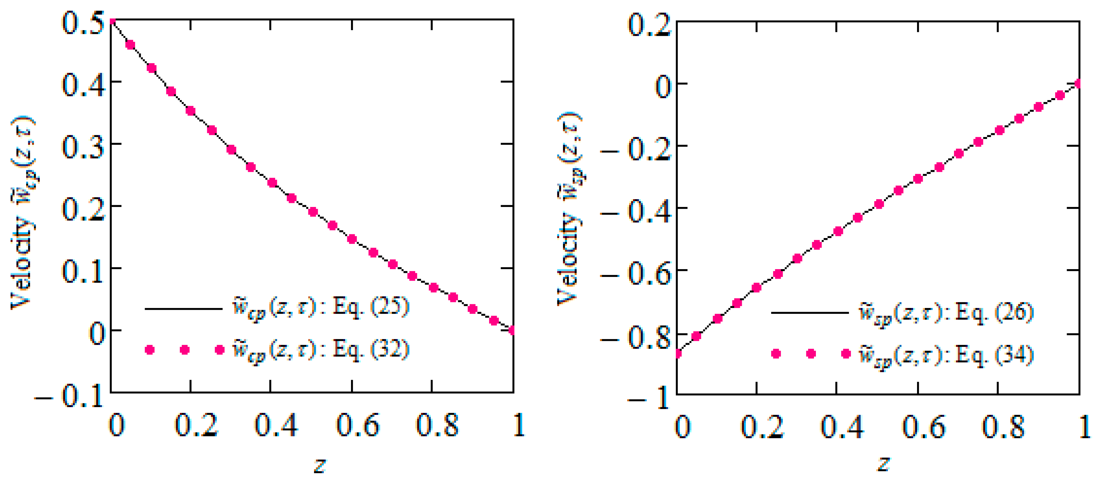
• Closed-form expressions are provided for the dimensionless steady-state velocity, shear stress and Darcy’s resistance of MHD modified Stokes’s problems for IGBFs through a porous medium. For validation, the fluid velocities are presented in equivalent forms.
• The obtained expressions can be immediately particularized to find similar solutions for Burgers, Oldroyd-B, Maxwell, second-grade and Newtonian fluids subject to same motions.
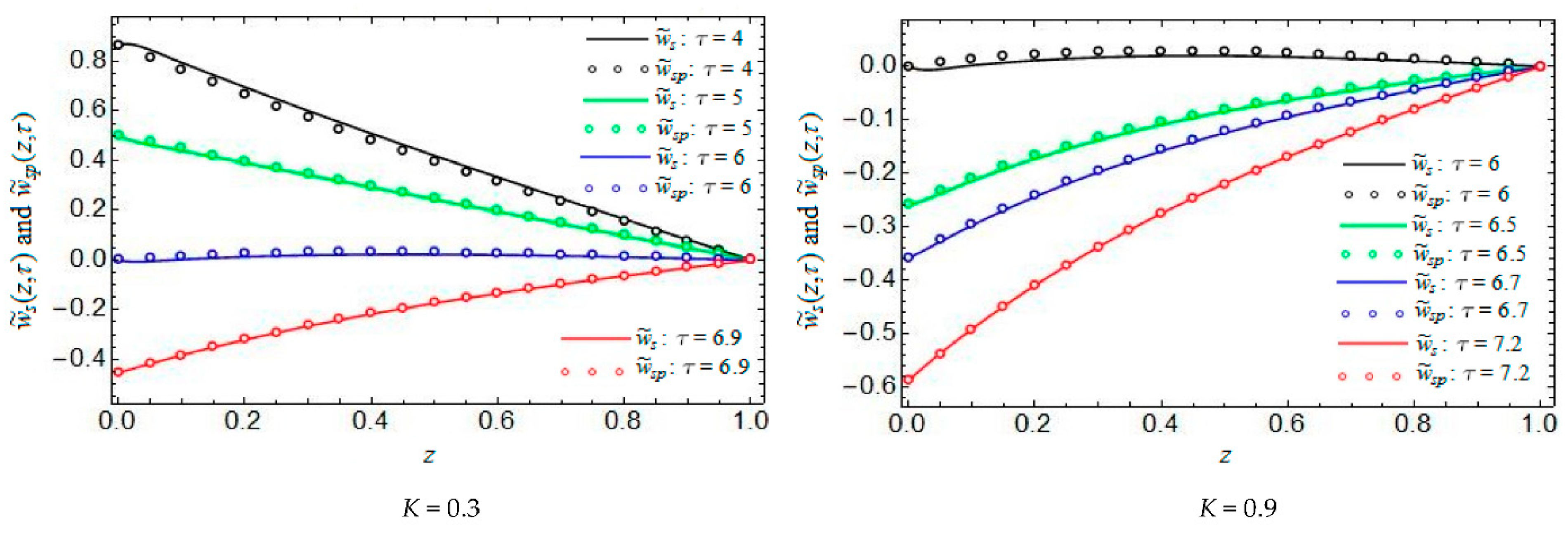
• Convergence of the starting velocities (numerical solutions) to their steady components is graphically proven, and the necessary time to reach a steady state is found.
• This time proportionally increases with the augmentation of the porous and magnetic parameters K and M, respectively. Consequently, the establishment of a steady state is more expeditiously achieved in the absence of a porous medium or a magnetic field.
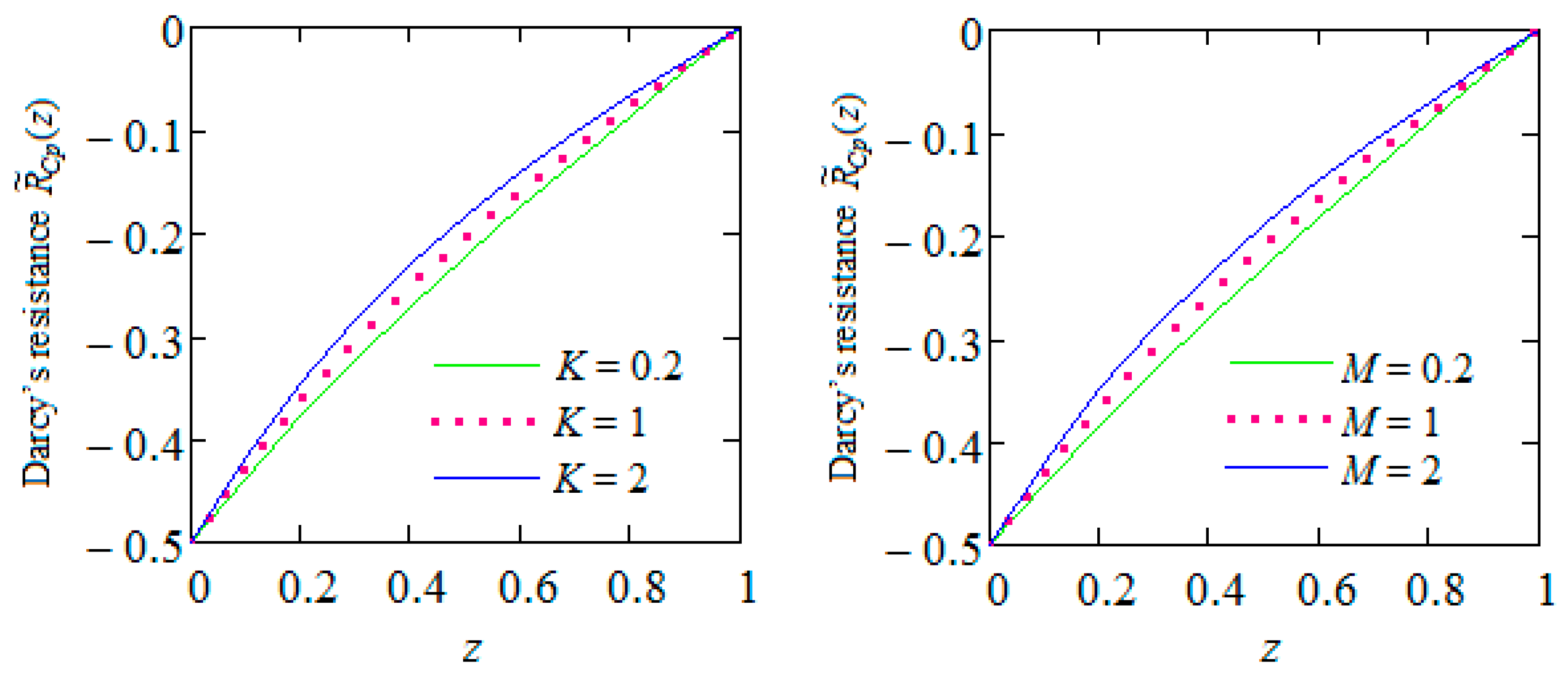
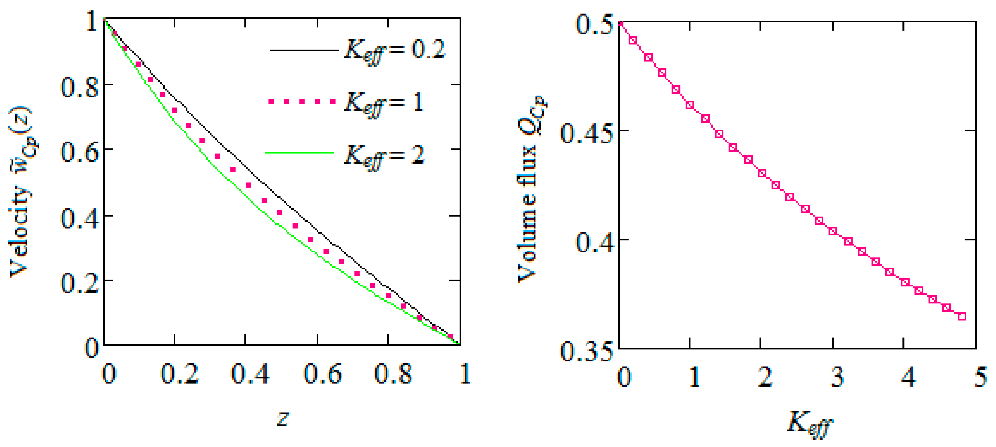
• The flow resistance of fluid exhibits a propensity to escalate in the presence of a porous medium or magnetic field. This results in a decelerated flow rate of the fluid within a porous medium or in the presence of a magnetic field.
• The governing equations for the fluid velocity and the non-trivial shear stress corresponding to the MHD motions of IGBFs between parallel plates are identical in form. Consequently, MHD motion problems with shear stress on the boundary can be solved for incompressible rate-type fluids.

References

1. Fetecau, C.; Hayat, T.; Fetecau, C. Seady-state solutions for some simple flows of generalized Burgers fluids. Int. J. Non-Linear Mech. 2006, 41, 880–887. [Google Scholar] [CrossRef]
2. Ravindran, P.; Krishnan, J.M.; Rajagopal, K.R. A note on the flow of a Burgers’ fluid in an orthogonal rheometer. Int. J. Eng. Sci. 2004, 42, 1973–1985. [Google Scholar] [CrossRef]
3. Zheng, L.C.; Zhao, F.F.; Zhang, X.X. An exact solution for an unsteady flow of a generalized Burgers’ fluid induced by an accelerating plate. Int. J. Nonlinear Sci. Numer. Simul. 2010, 11, 457–464. [Google Scholar] [CrossRef]
4. Jamil, M. First problem of Stokes for generalized Burgers’ fluids. Int. Sch. Res. Netw. ISRN Math. Phys. 2012, 2012, 831063. [Google Scholar] [CrossRef]
5. Fetecau, C.; Fetecau, C.; Akhtar, S. Permanent solutions for some axial motions of generalized Burgers fluids in cylindrical domains. Ann. Acad. Rom. Sci. Ser. Math. Appl. 2015, 7, 271–284. [Google Scholar]
6. Khan, I.; Hussanan, A.; Salleh, M.Z.; Tahar, R.M. Exact solutions of accelerated flows for a generalized Burgers’ fluid, I: The case. In Proceedings of the 4th International Conference on Computer Science and Computational Mathematics (ICCSCM 2015), Langkawi, Malaysia, 7–8 May 2015; pp. 47–52. [Google Scholar]
7. Tong, D. Starting solutions for oscillating motions of a generalized Burgers’ fluid in cylindrical domains. Acta Mech. 2010, 214, 395–407. [Google Scholar] [CrossRef]
8. Kiema, D.W.; Manyonge, W.A.; Bitok, J.K.; Adenyah, R.K.; Barasa, J.S. On the steady Couette flow between two infinite parallel plates in an uniform transverse magnetic field. J. Appl. Math. Bioinform. 2015, 5, 87–99. [Google Scholar]
9. Sultan, Q.; Nazar, M.; Imran, M.; Ali, U. Flow of generalized Burgers fluid between parallel walls induced by rectified sine pulses stress. Bound. Value Probl. 2014, 2014, 152. [Google Scholar] [CrossRef]
10. Sultan, Q.; Nazar, M. Flow of generalized Burgers’ fluid between side walls induced by sawtooth pulses stress. J. Appl. Fluid Mech. 2016, 9, 2195–2204. [Google Scholar] [CrossRef]
11. Khan, M.; Malik, R.; Anjum, A. Exact solutions of MHD second Stokes’ flow of generalized Burgers fluid. Appl. Math. Mech. Engl. Ed. 2015, 36, 211–224. [Google Scholar] [CrossRef]
12. Abro, K.A.; Hussain, M.; Baig, M.M. Analytical solution of magnetohydrodynamics generalized Burgers’ fluid embedded with porosity. Int. J. Adv. Appl. Sci. 2017, 4, 80–89. [Google Scholar] [CrossRef]
13. Alqahtani, A.M.; Khan, I. Time-dependent MHD flow of non-Newtonian generalized Burgers’ fluid (GBF) over a suddenly moved plate with generalized Darcy’s law. Front. Phys. 2020, 7, 214. [Google Scholar] [CrossRef]
14. Hussain, M.; Qayyum, M.; Afzal, S. Modeling and analysis of MHD oscillatory flows of generalized Burgers’ fluid in a porous medium using Fourier transform. J. Math. 2022, 2022, 2373084. [Google Scholar] [CrossRef]
15. Fetecau, C.; Morosanu, C. Steady state solutions of MHD Stokes problems for generalized Burgers fluids through porous media. Bul. Instit. Polit. Iasi 2023, submitted.
16. Rajagopal, K.R.; Saccomandi, G.; Vergori, L. Unsteady flows of fluids with pressure dependent viscosity. J. Math. Anal. Appl. 2013, 404, 362–372. [Google Scholar] [CrossRef]
17. Cramer, K.R.; Pai, S.I. Magnetofluid Dynamics for Engineers and Applied Physicists; McGraw-Hill: New York, NY, USA, 1973. [Google Scholar]
18. Prusa, V. Revisiting Stokes first and second problems for fluids with pressure-dependent viscosities. Int. J. Eng. Sci. 2010, 48, 2054–2065. [Google Scholar] [CrossRef]
19. Sneddon, I.N. Fourier Transforms; McGraw Hill, Book Company, Inc.: New York, NY, USA; Toronto, ON, Canada; London, UK, 1951. [Google Scholar]
20. Joseph, D.D. Fluid Dynamics of Viscoelastic Liquids; Springer-Verlag: New York, NY, USA, 1990. [Google Scholar]
21. Erdogan, M.E. On the unsteady unidirectional flows generated by impulsive motion of a boundary or sudden application of a pressure gradient. Int. J. Non-Linear Mech. 2002, 37, 1091–1106. [Google Scholar] [CrossRef]
Figure 1. Diagrams of the velocities w ˜ c p ( z , τ ) and w ˜ s p ( z , τ ) given by Equations (25) and (32) and (26) and (34), respectively, for α = 0.7 ,     β = 0.6 ,     γ = 0.5 ,     δ = 0.4 ,     ω = π / 6 ,     M = 0.8 and τ = 10 .
Dynamics 03 00044 g001
Figure 2. Equivalence of expressions of w ˜ C p ( z ) given by Equations (51) and (54) for two values of the effective permeability K e f f .
Dynamics 03 00044 g002
Figure 3. Convergence of w ˜ c ( z , τ ) (numerical solutions) with w ˜ c p ( z , τ ) for α = 0.7 ,   β = 0.6 ,   γ = 0.5 ,   δ = 0.4 ,   ω = π / 6 ,     M = 0.8 , two values of K and increasing values of time τ .
Dynamics 03 00044 g003
Figure 4. Convergence of w ˜ c ( z , τ ) (numerical solutions) with w ˜ c p ( z , τ ) for α = 0.7 ,   β = 0.6 ,   γ = 0.5 ,   δ = 0.4 ,   ω = π / 4 ,   K = 0.1 , two values of M and increasing values of time τ .
Dynamics 03 00044 g004
Figure 5. Convergence of w ˜ s ( z , τ ) (numerical solutions) with w ˜ s p ( z , τ ) for α = 0.7 ,   β = 0.6 ,   γ = 0.5 ,   δ = 0.4 ,   ω = π / 6 ,   M = 0.8 , two values of K and increasing values of time τ .
Dynamics 03 00044 g005
Figure 6. Convergence of w ˜ s ( z , τ ) (numerical solutions) with w ˜ s p ( z , τ ) for α = 0.7 ,   β = 0.6 ,   γ = 0.5 ,   δ = 0.4 ,   ω = π / 4 ,   K = 0.1 , two values of M and increasing values of time τ .
Dynamics 03 00044 g006
Figure 7. The time variations of the mid plane velocities w ˜ c p ( 1 / 2 , τ ) and w ˜ s p ( 1 / 2 , τ ) for α = 0.7 ,   β = 0.6 ,   γ = 0.5 ,   δ = 0.4 ,   ω = π / 12 ,   M = 0.8 and increasing values of K.
Dynamics 03 00044 g007
Figure 8. The time variations of the mid plane velocities w ˜ c p ( 1 / 2 , τ ) and w ˜ s p ( 1 / 2 , τ ) for α = 0.7 ,   β = 0.6 ,   γ = 0.5 ,   δ = 0.4 ,   ω = π / 12 ,   K = 0.5 and increasing values of M.
Dynamics 03 00044 g008
Figure 9. Variations in Darcy’s resistance R ˜ C p ( z ) from Equation (53) for α = 0.7 ,     β = 0.6 ,     γ = 0.5 ,   δ = 0.4 ,     M = 0.8 with three values of K and K = 0.5 with three values of M.
Dynamics 03 00044 g009
Figure 10. Influence of the effective permeability K e f f on the fluid velocity w ˜ C p ( z ) given by Equation (51) and the steady volume flux Q C p given by Equation (56).
Dynamics 03 00044 g010
Disclaimer/Publisher’s Note: The statements, opinions and data contained in all publications are solely those of the individual author(s) and contributor(s) and not of MDPI and/or the editor(s). MDPI and/or the editor(s) disclaim responsibility for any injury to people or property resulting from any ideas, methods, instructions or products referred to in the content.