The Dynamics of a Turning Ship: Mathematical Analysis and Simulation Based on Free Body Diagrams and the Proposal of a Pleometric Index

Abstract

This study attempts to shed new light on the dynamics of a turning ship using the principles of free body diagrams (FBDs). Unexpectedly, the literature gap is defined by incomplete and flawed FBDs. The method behind this new approach involves the FBD of a turning ship, with all the essential forces included, namely propulsive force, sideward thruster force (producing the initial turning moment), drag force, lift force, centrifugal force, inertial force, and hydrodynamic force couple. From these forces, the force and moment equations are derived. The accelerations are calculated from the force and moment equilibria to simulate the dynamics from input parameters such as mass m, length L, draught D, and fluid density ρ. The turning dynamics are explained in terms of velocities, accelerations, forces, and moments, based on two conditions: flat and steep angles of attack (AoA) and long and short turning radii R. A critical result is the proportionality of lift and centrifugal forces, leading to the proposal of a pleometric index (m·L^–2·D^–1·ρ^–1), which is nonlinearly proportional to the product of AoA and R/L, characterising the dynamics of a turning ship. The FBD approach of this study also identified missing databases required for accurate simulation of turning dynamics, such as drag and lift coefficients of different hull geometries.

1. Introduction

This study attempts to shed new light on the dynamics of a turning ship using the principles of free body diagrams (FBD). The purpose of an FBD is six-fold:

(1)

to provide a starting point for any mechanical analysis of forces (including their measurement);

(2)

to carefully isolate the FDB from its environment, identifying the location of the contact forces and their centre of pressure (COP), as well as the placement of contact sensors (force, pressure) for subsequent instrumentation at the interface of the FBD and its environment;

(3)

to include all forces acting on the FBD, which must be in equilibrium (the FBD is considered rigid);

(4)

although not part of the definition and therefore rarely mentioned in the textbooks, to consider the moments and their equilibrium;

(5)

to formulate the equilibrium equations (forces and moments) and calculate the magnitude and position (COP) of the contact forces, as well as accelerations, velocities, and displacements from resulting differential equations when the FBD is dynamic and not static;

(6)

to identify unknown parameters within the equilibrium equations and design tests to determine these parameters experimentally.

The best way to understand the importance of FBDs is to cite Shames [1] (p. 152):

‘I have found through many years of experience that the absence of a FBD in a student’s work on a particular problem signifies that there will most likely be errors in the analysis of the problem, or, even worse, the student does not have a good grasp of the problem’.

FBDs are found more commonly in engineering rather than in physics, and apply d’Alembert’s principle [2], that is, the ‘virtual’ inertial force, F_I, which corresponds to the product of mass and acceleration.

Surprisingly, FBDs are not common in ship dynamics, as the following literature review shows.

Several publications, including marine textbooks dealing with ship manoeuvres and hydrodynamic forces, did not include FBDs at all, such as Triantafyllou and Hover [3], Lewandowski [4], Newman [5], and Shuai et al. [6]. Kijima et al. [7] applied the equations of a rigid body in two dimensions, that is, forces in x- and y-directions, and moments about the z-axis; however, they did not depict any FBDs. Perera [8] (p. 3, Figure 1) dealt with the pivot point of a ship, but did not show any FBDs, and offered kinematic vector diagrams of velocities and accelerations.

Inoue et al. [9] (p. 113, Figure 2.1) showed a simple FBD of a ship with two general forces in x- and y-directions and a general moment about the z-axis. The two unspecific force vectors were not in equilibrium (nor was the moment), which means that the force equilibrium of the FBD was not established. The simple FBD of Inoue et al. [9] dominated the subsequent publications such as:

• Yoshimura [10] (p. 42, Figure 2), [11] (p. 78, Figure 1), [12] (p. 1, Figure 1), who also added the corresponding equations of motion;
• Pérez and Clemente [13] (p. 519, Figure 1);
• Carreño et al. [14] (p. 81, Figure 11), [15] (p. 28, Figure 1), [16] (p. 101, Figure 3), who, in the latter two publications [15,16] added the equations of a rigid body in two dimensions, that is, forces in x- and y-directions, and moment about the z-axis;
• Liu [17] (p. 109, Figure 5.6), who added the equations shown in [15];
• Huang and Wang [18] (p. 2251, Figure 1) showed an FBD, specifically labelled ‘free body diagram’, similar to [9], but also added rudder forces; furthermore, they listed the three equations of motion similar to [15], decomposing the x- and y-forces into propulsion, rudder and (hydrodynamic) hull resistance forces.
• The International Towing Tank Conference Association [19] (p. 11, Figure 3e,f) showed another simple FBD of a ship with two forces in x- and y-directions, specified as ‘hydrodynamic forces’, not in equilibrium with any other force vector. Their equations of motion [19] (p. 9, Equation (1)) included further forces, presumably applied ones, as well as inertial forces, that were not shown in their incomplete FBD.

Ji and Huang [20] (p. 2, Figure 2) showed a rudimentary FBD with a non-specific force and a ‘disturbance force’; these forces were not in equilibrium. Bowles [21] (p. 4, Figure 2) depicted an FBD, correctly called ‘partial’ FBD because the forces are not balanced, and included the specific forces of rudder (steering force), sideward hull resistance, and centrifugal force. The ABS (American Bureau of Shipping [22]) (p. 58, Figure 4) provides another incomplete FBD, indicating thrust (propulsion), rudder, lift and drag forces. Cheirdaris [23] (p. 20, Figures 2–9) shows a ‘hull lift‘ vector in a turning ship diagram. The force diagram of Halpern [24] shows a rudder force, drag force, and ‘centripetal’ hull force, the latter perpendicular to the ship’s movement [24] (p. 3, bottom figure), and a single ‘centripetal’ hull force almost perpendicular to the ship’s velocity vector and pointing to the rotation centre of the turn [24] (p. 6, bottom fig.). This ‘centripetal’ hull force appears to be the sideward hydrodynamic lift force, not to be confused with the (missing) centrifugal force. The force vector diagrams of references [23,24] are still incomplete free body diagrams.

Benedict [25] offers a more comprehensive force analysis of a turning ship than the previous literature, but his FBD is still incomplete. All the forces included are perpendicular to the ship’s roll axis, in particular the rudder force, the centrifugal force, the hydrodynamic drag force (‘lift’ force), and an unspecified ‘damping’ force. In addition, Benedict [25] compares a turning ship to an aerofoil.

In this context, Matusiak [26] (p. 29) mentions that ‘the inflow to the hull resembles the flow over a low aspect ratio aerofoil set at angle of attack β. Angle β is actually a drift angle of the ship’. Consequently, a lift force develops, originating from a ‘point N located between the stem … and mid-ship’ [26] (p. 29; p. 28, Figure 5.1). This ‘point N’ denotes the hydrodynamic centre of pressure.

Based on the literature gap identified above, specifically the lack of detailed and complete FBDs being in force equilibrium, the aim of this study is to plot the FBDs of a ship before and during turning (transient phase and steady state/steady turning mode), to derive the force and moment equations directly from the FBDs, and to evaluate the results of the turning dynamics from different aspects.

2. Methods

2.1. Free Body Diagrams and Mathematical Modelling of a Turning Ship

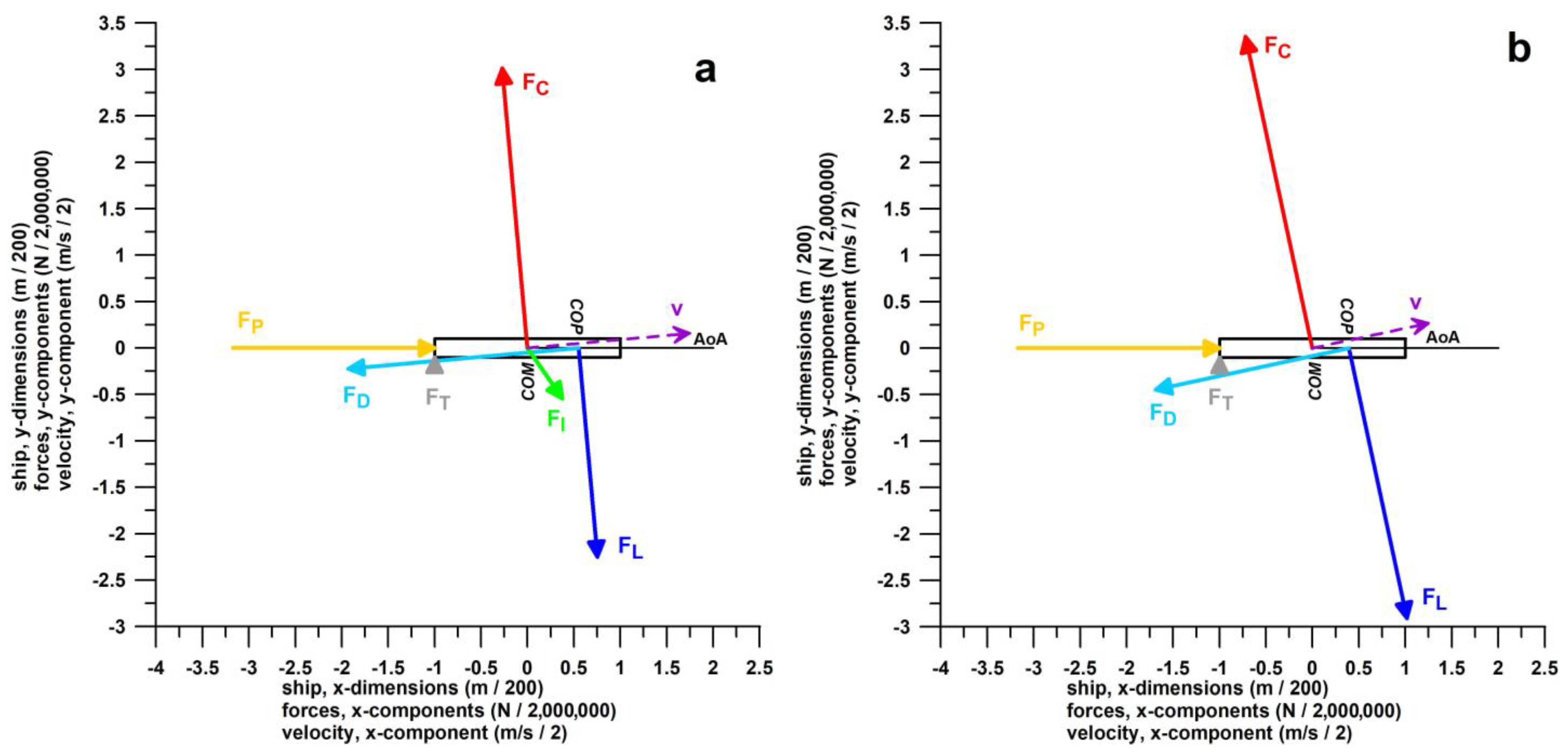
The body coordinate system (BCS; Figure 1a,b) of the FBD to be used in this analysis is as follows: x: aligned with the roll axis, pointing towards the bow; y: to the left (port side); and z: upward. For modelling purposes, the FBD of the ship is reduced to a vertical flat plate with a length-to-beam ratio > 6.8. The centre of mass (COM) is assumed at the centroid of the plate.

The forces (Figure 1a,b) included in the analysis were four applied forces originating from different COPs, two forces originating from the COM, and one force couple:

(1)

propulsive force, F_P, acting in the direction of +x with its COP at the stern;

(2)

thruster force, F_T, perpendicular to F_P, in the direction of ±y and having its COP at stern;

(3)

hydrodynamic drag force, F_D, opposed to the ship’s velocity vector, originating from the hydrodynamic COP;

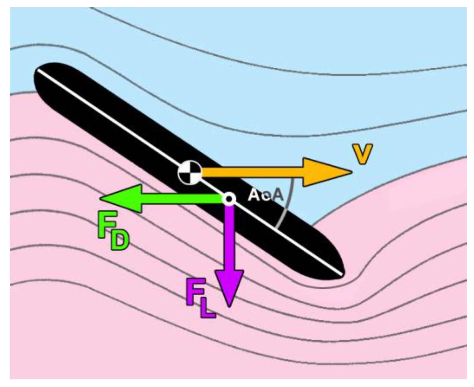
(4)

hydrodynamic lift force, F_L, acting perpendicular to the ship’s velocity vector and centripetally sideways (Figure 2), originating from the hydrodynamic COP;

(5)

centrifugal force, F_C, perpendicular to the tangent at the ships trajectory curve, and thus pointing away from the centre of rotation (COR), originating from the COM;

(6)

inertial force, F_I, originating from the COM;

(7)

hydrodynamic force couple created by the rotation of the ship, producing a free moment.

Forces (3)–(6) were resolved into their x- and y-components. The gravitational force was not included since it does not act in the xy-plane.

The moments included in the analysis were those generated by the x- and y-components of forces (1)–(6) about a point, P, and the two free moments, one produced by the force couple 7, and the second created by product of angular acceleration and moment of inertia of the ship. Point P, about which the moment equilibrium is calculated, can be the COM, COP, COR, or any other point, since the moment equilibrium of a FBD is a free moment of zero magnitude, provided the forces are in equilibrium. In this study, P = COM, which means that forces (or components of forces) in x-direction have a zero moment arm.

Figure 1. Free body diagrams (FBDs) of a ship turning clockwise; (a) transient phase, at the peak of the angular acceleration; (b) steady state; F_P = propulsive force, F_T = stern thruster force, F_D = drag force, F_L = lift force; F_C = centrifugal force, F_I = inertial force, COM = centre of mass (origin of F_C and F_I), COP = centre of pressure (origin of F_D and F_L), AoA = angle of attack; v = translational velocity (presented for clarity only, not a part of the FBD).

Figure 1. Free body diagrams (FBDs) of a ship turning clockwise; (a) transient phase, at the peak of the angular acceleration; (b) steady state; F_P = propulsive force, F_T = stern thruster force, F_D = drag force, F_L = lift force; F_C = centrifugal force, F_I = inertial force, COM = centre of mass (origin of F_C and F_I), COP = centre of pressure (origin of F_D and F_L), AoA = angle of attack; v = translational velocity (presented for clarity only, not a part of the FBD).

The limitations of this approach are the lack of hydrodynamic data to calculate forces (3), (4), and (7), in particular the drag (C_D) and lift (C_L) coefficients, and the position of the hydrodynamic COP, and the drag coefficient of a rotating ship (yaw). Aerodynamic data are available, particularly for symmetrical and cambered streamlined bodies such as symmetrical aerofoils, cambered aerofoils, flat plates with AoA less than the stall angle, and teardrop shapes without or with Kamm tails. Although the flow of a fluid along the hull is comparable to the flow pattern of a flat plate (Figure 2), the flow of a fluid across the hull of a turning ship happens only unilaterally, namely below the keel but evidently not above the waterline. The shape of the hull—for example, round-, flat-, or V-bottom—is another factor that influences its hydrodynamic behaviour.

Figure 2. Fluid flow streamlines around the hull of a ship turning clockwise; the blue area corresponds to the reduced flow rate and higher pressure side and the red area to the increased flow rate and lower pressure side; the streamline separating the blue and red areas is the stagnation streamline, passing through front and back stagnation points (flow separation point [rear stagnation point] may be further upstream); v: instantaneous velocity vector of the centre of mass; F_D: drag force originating from the hydrodynamic centre of pressure; F_D: lift force; AoA: angle of attack.

Figure 2. Fluid flow streamlines around the hull of a ship turning clockwise; the blue area corresponds to the reduced flow rate and higher pressure side and the red area to the increased flow rate and lower pressure side; the streamline separating the blue and red areas is the stagnation streamline, passing through front and back stagnation points (flow separation point [rear stagnation point] may be further upstream); v: instantaneous velocity vector of the centre of mass; F_D: drag force originating from the hydrodynamic centre of pressure; F_D: lift force; AoA: angle of attack.

To overcome these limitations, C_D, C_L, and the position of the COP (Figure 3) were modelled based on the generic forms of their functions of the angle of attack AoA. The latter corresponds to the drift angle of a turning ship. These functions, Equations (1)–(3), serve to clarify the dynamic trend of the mutually influencing in- and output parameters, but not to model specific ships, whose hydrodynamic data are unknown. For example, how does changing the mass (displacement; input parameter) of a ship affect the turning circle radius (output parameter)? The generic functions of C_D, C_L, and COP versus AoA were derived from the wind tunnel data gathered by Ortiz et al. [27], who studied flat plates at different aspect ratios. In the absence of experimental hydrodynamic data, the data in [27] are sufficient for modelling free body diagrams. From the data in [27], the equations of C_D, C_L, and the position of the COP as a function of the AoA (up to 50°; Figure 3) were derived by non-linear fitting:

$$C_D=-6.667\times {10}^{-6} \mathrm{A}\mathrm{o}{\mathrm{A}}^3+6.793\times {10}^{-4}\mathrm{A}\mathrm{o}{\mathrm{A}}^2+7.011\times {10}^{-4} \mathrm{A}\mathrm{o}\mathrm{A}+1.031\times {10}^{-1}$$

(1)

$$C_L=-3.497\times {10}^{-7} \mathrm{A}\mathrm{o}{\mathrm{A}}^4+1.702\times {10}^{-5} \mathrm{A}\mathrm{o}{\mathrm{A}}^3-3.322\times {10}^{-5} \mathrm{A}\mathrm{o}{\mathrm{A}}^2+2.150\times {10}^{-2} \mathrm{A}\mathrm{o}\mathrm{A}+5.245\times {10}^{-3},$$

(2)

$$COP=-3.810\times {10}^{-6} \mathrm{A}\mathrm{o}{\mathrm{A}}^3+5.877\times {10}^{-4} \mathrm{A}\mathrm{o}{\mathrm{A}}^2-3.186\times {10}^{-2} \mathrm{A}\mathrm{o}\mathrm{A}+7.012\times {10}^{-1},$$

(3)

where COP is expressed as a fraction of half the ship’s length (L/2), with positive COP values between COM and bow.

The drag and lift forces, F_D and F_L, were calculated from:

$$F_D=\mathsf{½} \rho C_D A v^2,$$

(4)

$$F_L=\mathsf{½} \rho C_L A v^2,$$

(5)

where ρ denotes the fluid density, A is the area of the flat plate (product of length L and draught D of a ship), and v is the velocity of the ship. Reference [19] (p. 9, Equations (2) and (3)) uses the same area parameter in their hydrodynamic equations, namely the product of ‘mean draft’ and ‘ship length’, comparable to the reference area in flat plates [27] and aerofoils (or any streamlined body in general). Forces X and Y in reference [19] (p. 11, Figure 3e,f) correspond to the drag and lift forces, F_D and F_L, and coefficients X’ and Y’ in reference [19] correspond to the drag and lift coefficients, C_D and C_L.

Figure 3. Drag coefficient C_D, lift coefficient C_L, and relative position of the centre of pressure COP versus the angle of attack AoA (drift angle), based on the data from [27]; the position of the COP at 0.7 (AoA = 0°) means that the COP is located 0.7·(L/2)·100% in front of the ship’s centroid, where L is the length of the ship (‘length between perpendiculars’).

Figure 3. Drag coefficient C_D, lift coefficient C_L, and relative position of the centre of pressure COP versus the angle of attack AoA (drift angle), based on the data from [27]; the position of the COP at 0.7 (AoA = 0°) means that the COP is located 0.7·(L/2)·100% in front of the ship’s centroid, where L is the length of the ship (‘length between perpendiculars’).

Note that for bluff bodies (sphere, cylinder, flat plate with AoA of 90°, etc.), the reference area A is the frontal area, projected onto the direction of the fluid flow, i.e., the area A is perpendicular to the fluid flow. In streamlined bodies (symmetrical aerofoils, cambered aerofoils, flat plates with AoA smaller than the stall angle, teardrop shapes with or without Kamm tails, ships, etc.), the reference area A is not perpendicular to the main fluid flow (with the exception of circular flows at the edges) but parallel to the fluid flow. The aspect ratio of a streamlined body is length to width, where the width is measured in the direction of the flow, and the length is perpendicular to the direction of the flow. The length of a ship corresponds to the width in the aspect ratio equation.

The moments M_D,L of the y-components of F_D and F_L about the COM were calculated as follows

$$M_{D,L}=\left(F_{Dy}+F_{Ly}\right) \mathrm{C}\mathrm{O}\mathrm{P}\frac{L}{2}$$

(6)

The centrifugal force F_C was calculated from

$$F_C=m R {\omega }^2,$$

(7)

where m denotes the mass of the ship (including hydrodynamic added mass), ω denotes the angular velocity, and R corresponds to the turning radius, calculated from

$$R=\frac{v}{\omega }$$

(8)

The components of the inertial force F_I resulted from the force equilibria in x- and y-directions:

$$F_P+F_{Dx}+F_{Lx}+F_{Cx}+F_{Ix}=0,$$

(9)

and

$$F_T+F_{Dy}+F_{Ly}+F_{Cy}+F_{Iy}=0,$$

(10)

where F_P is always positive in the BCS, and the signs of all other forces or components thereof depend on the dynamic scenarios, including the turning direction.

The translational accelerations of the ship, a_x and a_y, resulting from F_Ix and F_Iy, are

$$a_{x,y}=-\frac{F_{Ix,y}}{m}$$

(11)

The hydrodynamic force couple that opposes the force couple of F_C and F_L and the moment of F_T is explained as follows. The instantaneous motion of a turning ship can be viewed as a combined motion consisting of two individual motions (Figure 4a): (1) linear motion along the translational velocity vector v (Figure 4b), and (2) rotational motion about the COM (Figure 4c,d). The linear motion subjects the ship to drag and lift (F_D and F_L; Figure 4b), whereas the rotational motion churns the sea and produces hydrodynamic pressure on both sides of the ship (Figure 4c), resulting in a force couple (Figure 4d). Evidently, the maximum water pressure occurs at the bow and stern (Figure 4c), that is, at a distance of L/2 (half the ship’s length) from the COM, where the tangential velocity generated by ω is at its maximum. Conversely, the tangential velocity at the COM is zero. The tangential velocity decreases linearly from each of the two ends of the ship towards the COM, whereas the water pressure (Figure 4c) decreases non-linearly following a quadratic function (cf. Equation (4)). This water pressure can be expressed by a single force vector, F_D2, on either side of the COM (Figure 4d), resulting from integrating the water pressure over L/2 and originating from a centre of pressure (COP2).

Rotating one half of a flat plate of width w and length L/2 about a COR at one end of the flat plate (equivalent to the COM of a ship), then the local water pressure dF_D2 is

$$\mathrm{d}{F}_{D2}=0.5 \rho C_{D2} \mathrm{d}r w {v_t}^2,$$

(12)

where r is the distance from COM to bow or stern, that is, 0 ≤ r ≤ L/2; C_D2 is the drag coefficient applicable to the conditions shown in Figure 4c,d; and v_t is a function of ω, namely

$$v_t=\omega r.$$

(13)

Thus,

$$\mathrm{d}{F}_{D2}=0.5 \rho C_{D2} \mathrm{d}r w {\omega }^2 r^2,$$

(14)

Let c = 0.5 ρ C_D2 w, then

$$\mathrm{d}{F}_{D2}=c \mathrm{d}r {\omega }^2 r^2,$$

(15)

and

$$F_{D2}=c {\omega }^2 {\int }_0^{L/2}{r}^2 \mathrm{d}r.$$

(16)

Integrating r from 0 to L/2

$$F_{D2}=c {\omega }^2 {\left|\frac{r^3}{3}\right|}_0^{L/2}$$

(17)

and

$$F_{D2}=c {\omega }^2 \frac{{\left(L/2\right)}^3}{3}$$

(18)

To identify the relative position of COP2 between COR and L/2, we normalise Equation (18) to L/2:

$$F_{D2}=c {\omega }^2/3$$

(19)

If we integrate r in Equation (16) from 0 to COP2 and from COP2 to L/2 and equate the two partial F_D2 on either side of the COP2, we obtain the exact position of COP2. Rearranging Equation (17) and normalising to L/2:

$$\begin{gathered} c {\omega }^2 {\left|\frac{r^3}{3}\right|}_0^{\mathrm{C}\mathrm{O}\mathrm{P}2}=c {\omega }^2 {\left|\frac{r^3}{3}\right|}_{\mathrm{C}\mathrm{O}\mathrm{P}2}^1 \\ {\mathrm{C}\mathrm{O}\mathrm{P}2}^3-0=1-{COP2}^3 \\ \mathrm{C}\mathrm{O}\mathrm{P}2=2^{-\frac{1}{3}}\approx 0.7937. \end{gathered}$$

(20)

Therefore, COP2 is located at approximately 80% of L/2.

The moment created by the hydrodynamic forces on one half of the flat plate results from Equations (18) and (20)

$$M_{D2}=c {\omega }^2 \frac{{\left(\frac{L}{2}\right)}^3}{3} 2^{-\frac{1}{3}} \left(\frac{L}{2}\right)=c {\omega }^2\frac{{\left(\frac{L}{2}\right)}^4}{3·2^{\frac{1}{3}}}$$

(21)

The torque of the hydrodynamic force couple is then 2M_D2, which has the opposite direction of ω. The limitations of this approach are that one half of a rotating flat plate does not behave like a flat plate with fluid flow over all four sides. However, there will be fluid flow from one half to the other half, that is, from the high-pressure zone to the low-pressure zone. For modelling purposes, C_D2 is assumed to be constant.

The torque T generated by the moment of inertia I results from the moment equilibrium about the z-axis:

$$F_T\frac{L}{2}+\left(F_{Dy}+F_{Ly}\right) \mathrm{C}\mathrm{O}\mathrm{P}\frac{L}{2}+2M_{D2}+T=0.$$

(22)

The angular acceleration of the ship, α, resulting from T, is

$$\alpha =-\frac{T}{I}$$

(23)

where I denotes the moment of inertia (MoI) of the ship, that is, the product of its mass and radius of gyration squared.

In this study, the following forces were not considered: friction drag, aerodynamic forces (wind), wave forces, and disturbance forces [20], mainly due to the lack of data, but also to keep the forces acting on the FBD to the absolute minimum required. Compared to the literature review above, the FBD presented in this section is already more comprehensive than all the FBDs shown in the literature sources cited above.

Integration of the accelerations obtained from Equations (11) and (23) provides the translational and angular velocities v and ω, respectively. The COR is calculated from the radius R in Equation (8), which connects the COM to the COR, perpendicular to the vector of v. After the ship’s velocity, forces, and COR are calculated in the BCS, integrating v_x, v_y, and ω results in the ship’s COM movements in x- and y-directions (x_COM, y_COM) as well as the angular movement θ of the ship, respectively, in the global coordinate system (GCS). Subsequently, any vector (velocity, forces; positions of COM, COP, COR) is rotated from the BCS to the GCS from

$$X_{\mathrm{G}\mathrm{C}\mathrm{S}}=X_{\mathrm{BCS}}\cos \theta -Y_{\mathrm{BCS}}\sin \theta +x_{\mathrm{C}\mathrm{O}\mathrm{M}},$$

(24)

and

$$Y_{\mathrm{G}\mathrm{C}\mathrm{S}}=X_{\mathrm{BCS}}\sin \theta +Y_{\mathrm{BCS}}\cos \theta +y_{\mathrm{C}\mathrm{O}\mathrm{M}},$$

(25)

where X_BCS, Y_BCS, and Y_GCS, X_GCS are the coordinates in the BCS and the GCS, respectively.

2.2. Input Data and Scenarios for Simulation

The input variables required for the numerical simulation of the behaviour of a turning ship, modelled as a flat plate, were:

(a)

the drag coefficient C_D, the lift coefficient C_L, and the relative position of the centre of pressure COP as a function of the angle of attack AoA (drift angle), based on the data from Ortiz et al. [27], expressed as polynomial fit functions in Equations (1)–(3) and shown in Figure 3;

(b)

the mass m, length L, and draught D of ships to be simulated; and

(c)

the density ρ of seawater (1024 kg m ^–3).

The default data used as a starting point for the variation of the input data were approximately the same as the data on the characteristics of the Seawise Giant [28], particularly the following: mass (displacement, loaded) m = 5 × 10⁸–6.6 × 10⁸ kg; length L = 458 m; and draught D = 24.6 m. The simulation was performed by using Equations (1)–(25) and first systematically changing only a single variable (m, L, D, ρ; cf. Table 1), followed by randomly changing the combinations of m, L, and D (Monte Carlo method).

2.3. Validation of the Simulation with Experimental Data

Gug et al. [29] carried out turning tests with a training ship with the following characteristics: m = 6.418·10⁶ kg; length L = 104 m; and draught D = 5.9 m [29] (p. 2, Table 1), with an initial speed of 9 m/s [29] (p. 3, Table 2). Gug et al. [29] calculated the mean radii of the turning circle from the ship’s GPS-data, which were 163.28 m and 183.56 m on portside and starboard side, respectively [29] (p. 10, Table 7). The simulation was recalculated with the ship properties and initial speed provided by Gug et al. [29] as input data of the model, and the radius of the turning circle as well as the AoA were determined from the input data.

Table 1. The influence of the model input data on the angle of attack (AoA) and the turning radius (R); L: length (‘between perpendiculars’); D: draught; m: mass; ρ: density of fluid medium (seawater: 1024 kg/m³); the variation of the input data (bold font, columns 2–5) was divided into four categories: average increase or decrease, and maximum increase or decrease; the multipliers and divisors of the input data were selected to give the same AoA-data within each of the four categories (column 6); the R-data were not the same when L was varied (bold font, column 7) but higher or lower than expected; dividing R by L yields data that are the same in each of the four categories (column 8); in the product of AoA and R/L (rightmost column), the influence of AoA outweighs that of R/L; index 𐊬: pleometric index from Equation (33). For easier data identification, the cells of the table are highlighted in different colors, ranging from low to high values through the color spectrum across the color spectrum of blue, cyan, green, yellow and red.

Input Data	L (m)	D (m)	m (kg)	ρ (kg/m3)	AoA (°)	R (m)	R/L (-)	log AoA	log R/L	log index 𐊬	log (AoA·R/L)
m/4	458.5	24.6	164,247,068	1024	0.26	3292.1	7.18	−0.577	0.86	−1.51	0.28
4ρ	458.5	24.6	656,988,272	4096	0.26	3292.1	7.18	−0.577	0.86	−1.51	0.28
4D	458.5	98.4	656,988,272	1024	0.26	3292.1	7.18	−0.577	0.86	−1.51	0.28
2L	917	24.6	656,988,272	1024	0.26	6584.1	7.18	−0.577	0.86	−1.51	0.28
m/2	458.5	24.6	328,494,136	1024	1.03	1745.2	3.81	0.013	0.58	−1.21	0.59
2ρ	458.5	24.6	656,988,272	2048	1.03	1745.2	3.81	0.013	0.58	−1.21	0.59
2D	458.5	49.2	656,988,272	1024	1.03	1745.2	3.81	0.013	0.58	−1.21	0.59
1.4L	648.4	24.6	656,988,272	1024	1.03	2468.1	3.81	0.013	0.58	−1.21	0.59
default	458.5	24.6	656,988,272	1024	4.01	1011	2.21	0.603	0.34	−0.91	0.95
2m	458.5	24.6	1,313,976,544	1024	11.66	743.8	1.62	1.067	0.21	−0.61	1.28
ρ/2	458.5	24.6	656,988,272	512	11.66	743.8	1.62	1.067	0.21	−0.61	1.28
D/2	458.5	12.3	656,988,272	1024	11.66	743.8	1.62	1.067	0.21	−0.61	1.28
L/1.4	324.2	24.6	656,988,272	1024	11.66	525.9	1.62	1.067	0.21	−0.61	1.28
4m	458.5	24.6	2,627,953,088	1024	21.94	644.6	1.41	1.341	0.15	−0.30	1.49
ρ/4	458.5	24.6	656,988,272	256	21.94	644.6	1.41	1.341	0.15	−0.30	1.49
D/4	458.5	6.2	656,988,272	1024	21.94	644.6	1.41	1.341	0.15	−0.30	1.49
L/2	229.3	24.6	656,988,272	1024	21.94	322.3	1.41	1.341	0.15	−0.30	1.49

Table 1. The influence of the model input data on the angle of attack (AoA) and the turning radius (R); L: length (‘between perpendiculars’); D: draught; m: mass; ρ: density of fluid medium (seawater: 1024 kg/m³); the variation of the input data (bold font, columns 2–5) was divided into four categories: average increase or decrease, and maximum increase or decrease; the multipliers and divisors of the input data were selected to give the same AoA-data within each of the four categories (column 6); the R-data were not the same when L was varied (bold font, column 7) but higher or lower than expected; dividing R by L yields data that are the same in each of the four categories (column 8); in the product of AoA and R/L (rightmost column), the influence of AoA outweighs that of R/L; index 𐊬: pleometric index from Equation (33). For easier data identification, the cells of the table are highlighted in different colors, ranging from low to high values through the color spectrum across the color spectrum of blue, cyan, green, yellow and red.

Input Data	L (m)	D (m)	m (kg)	ρ (kg/m3)	AoA (°)	R (m)	R/L (-)	log AoA	log R/L	log index 𐊬	log (AoA·R/L)
m/4	458.5	24.6	164,247,068	1024	0.26	3292.1	7.18	−0.577	0.86	−1.51	0.28
4ρ	458.5	24.6	656,988,272	4096	0.26	3292.1	7.18	−0.577	0.86	−1.51	0.28
4D	458.5	98.4	656,988,272	1024	0.26	3292.1	7.18	−0.577	0.86	−1.51	0.28
2L	917	24.6	656,988,272	1024	0.26	6584.1	7.18	−0.577	0.86	−1.51	0.28
m/2	458.5	24.6	328,494,136	1024	1.03	1745.2	3.81	0.013	0.58	−1.21	0.59
2ρ	458.5	24.6	656,988,272	2048	1.03	1745.2	3.81	0.013	0.58	−1.21	0.59
2D	458.5	49.2	656,988,272	1024	1.03	1745.2	3.81	0.013	0.58	−1.21	0.59
1.4L	648.4	24.6	656,988,272	1024	1.03	2468.1	3.81	0.013	0.58	−1.21	0.59
default	458.5	24.6	656,988,272	1024	4.01	1011	2.21	0.603	0.34	−0.91	0.95
2m	458.5	24.6	1,313,976,544	1024	11.66	743.8	1.62	1.067	0.21	−0.61	1.28
ρ/2	458.5	24.6	656,988,272	512	11.66	743.8	1.62	1.067	0.21	−0.61	1.28
D/2	458.5	12.3	656,988,272	1024	11.66	743.8	1.62	1.067	0.21	−0.61	1.28
L/1.4	324.2	24.6	656,988,272	1024	11.66	525.9	1.62	1.067	0.21	−0.61	1.28
4m	458.5	24.6	2,627,953,088	1024	21.94	644.6	1.41	1.341	0.15	−0.30	1.49
ρ/4	458.5	24.6	656,988,272	256	21.94	644.6	1.41	1.341	0.15	−0.30	1.49
D/4	458.5	6.2	656,988,272	1024	21.94	644.6	1.41	1.341	0.15	−0.30	1.49
L/2	229.3	24.6	656,988,272	1024	21.94	322.3	1.41	1.341	0.15	−0.30	1.49

3. Results

3.1. Dynamic Parameters of a Turning Ship

The dynamic parameters are explained subsequently by comparing two conditions, namely the long (condition 1) and the short (condition 2) radius R of the turning circle. The graphs associated with conditions 1 and 2 are displayed side by side (Figure 5, Figure 6, Figure 7, Figure 8, Figure 9, Figure 10, Figure 11, Figure 12, Figure 13 and Figure 14). Condition 1 is associated with low mass m, and a large length L, draught D, and (water) density ρ (Table 1). Condition 2 is associated with large mass m, short length L, and small draught D, as well as low (water) density ρ (Table 1). The variation of ρ in Table 1 is only of theoretical interest to understand the individual influences of m, L, D, and ρ.

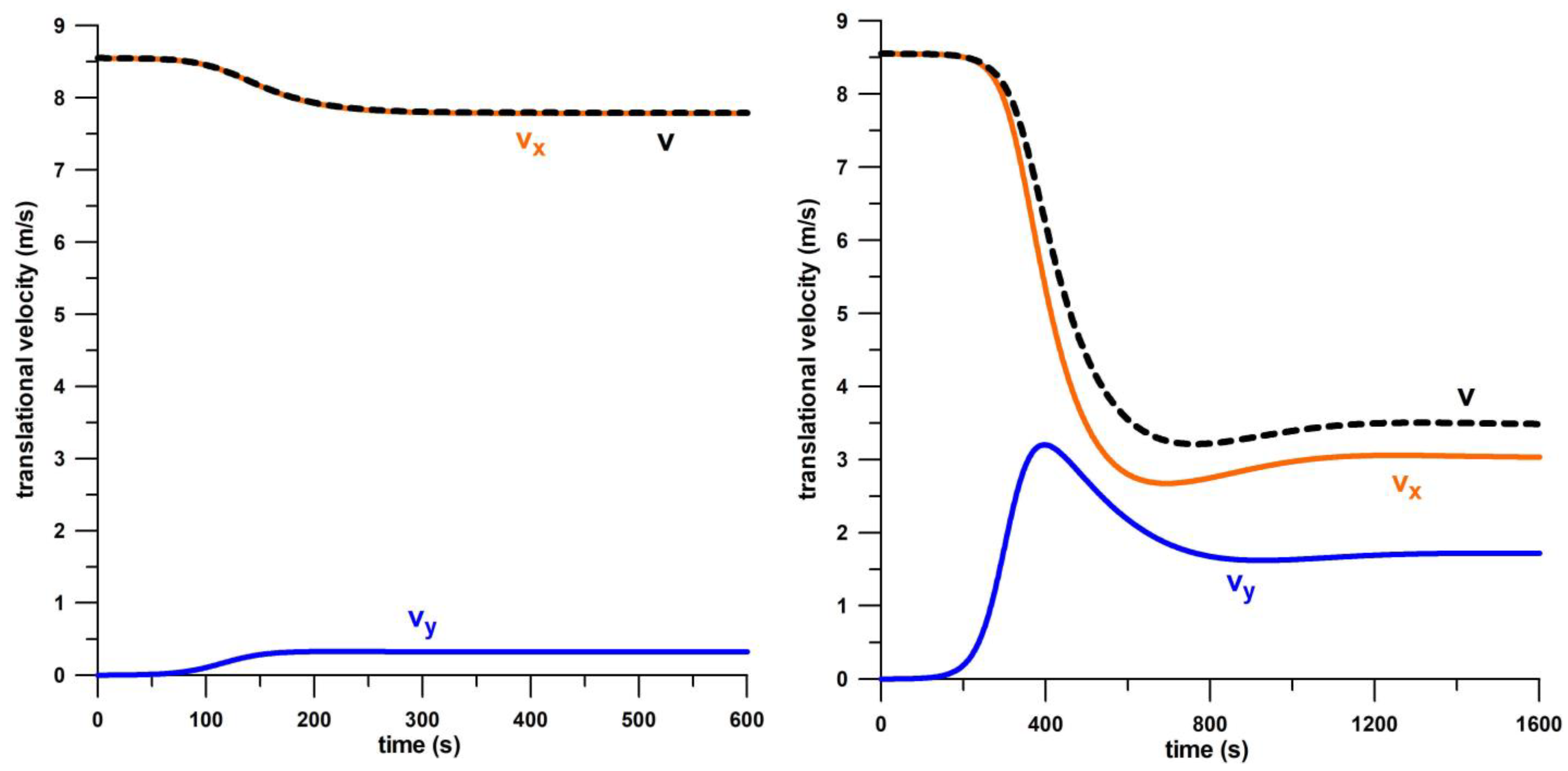
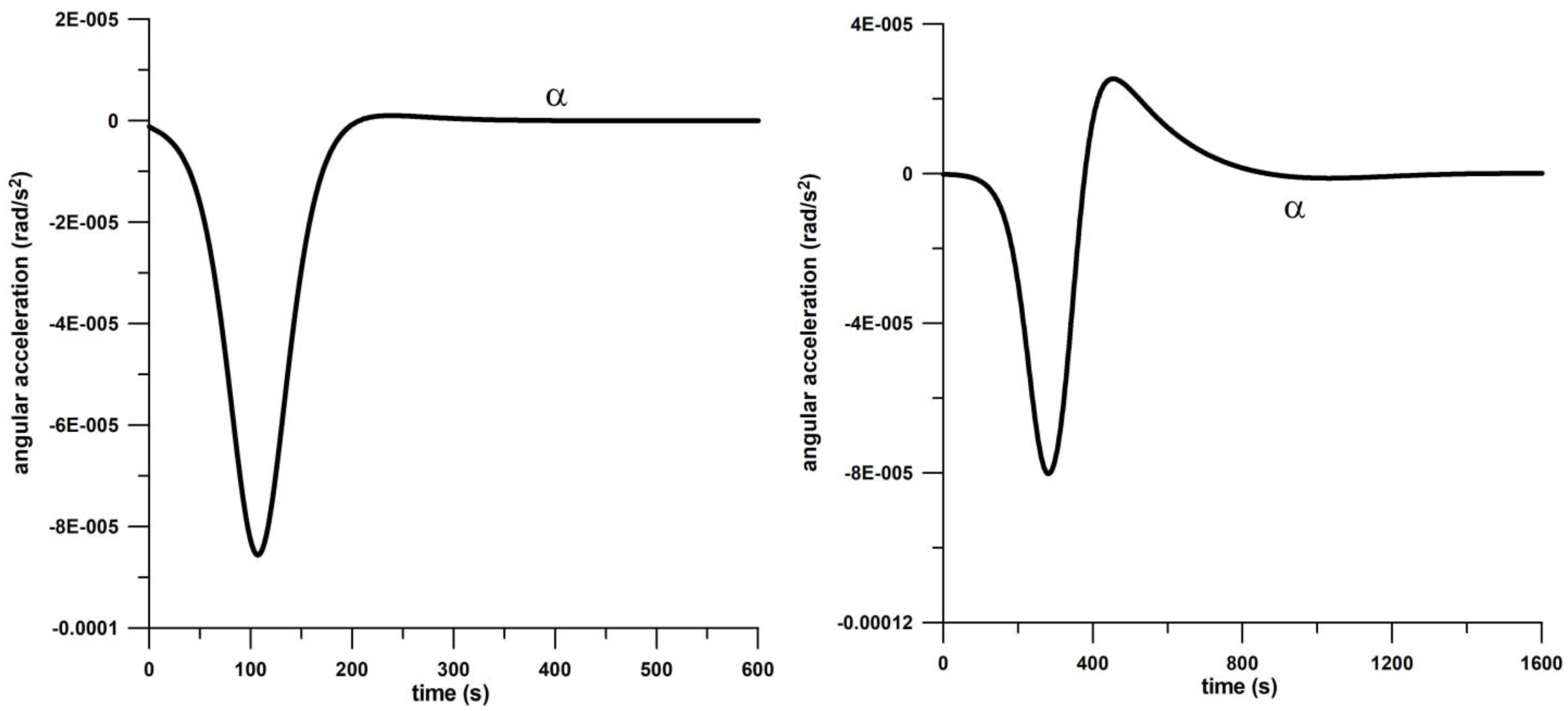
3.1.1. Velocities and Accelerations

The difference in translational velocity v (Figure 5) between conditions 1 and 2 is that v and its component v_x decrease more in condition 2; v_y increases more strongly and shows a clear overshoot. In contrast to the translational velocity, the patterns of the translational acceleration a (Figure 6) look the same in both conditions, although the component a_y is characterized by an undershoot (below zero) that follows the a_y-peak in condition 2. The translational acceleration a is zero in the steady state of turning. The angular velocity ω (Figure 7) decreases during the transient phase in both conditions; condition 2 shows a clear downward spike. The angular velocity ω is negative when the ship is turning clockwise. The angular acceleration α (Figure 8) shows a downward spike before returning to zero at steady state; in condition 2 this return to zero is interrupted by an upward spike (overshoot). In summary, the transient phase of condition 2 features clear spikes or over/undershoots resulting from opposing sudden changes in velocity or acceleration.

Figure 5. Translational velocity v (incl. x- and y-components) versus time, for conditions 1 (left) and 2 (right); conditions 1 and 2 relate to long and short radii of the turning circle, respectively (this principle applies to Figure 5, Figure 6, Figure 7, Figure 8, Figure 9, Figure 10, Figure 11, Figure 12, Figure 13 and Figure 14).

Figure 5. Translational velocity v (incl. x- and y-components) versus time, for conditions 1 (left) and 2 (right); conditions 1 and 2 relate to long and short radii of the turning circle, respectively (this principle applies to Figure 5, Figure 6, Figure 7, Figure 8, Figure 9, Figure 10, Figure 11, Figure 12, Figure 13 and Figure 14).

Figure 6. Translational acceleration a (incl. x- and y-components) versus time, for conditions 1 (left) and 2 (right).

Figure 6. Translational acceleration a (incl. x- and y-components) versus time, for conditions 1 (left) and 2 (right).

Figure 7. Angular velocity ω versus, for conditions 1 (left) and 2 (right).

Figure 7. Angular velocity ω versus, for conditions 1 (left) and 2 (right).

Figure 8. Angular acceleration α versus time, for conditions 1 (left) and 2 (right).

Figure 8. Angular acceleration α versus time, for conditions 1 (left) and 2 (right).

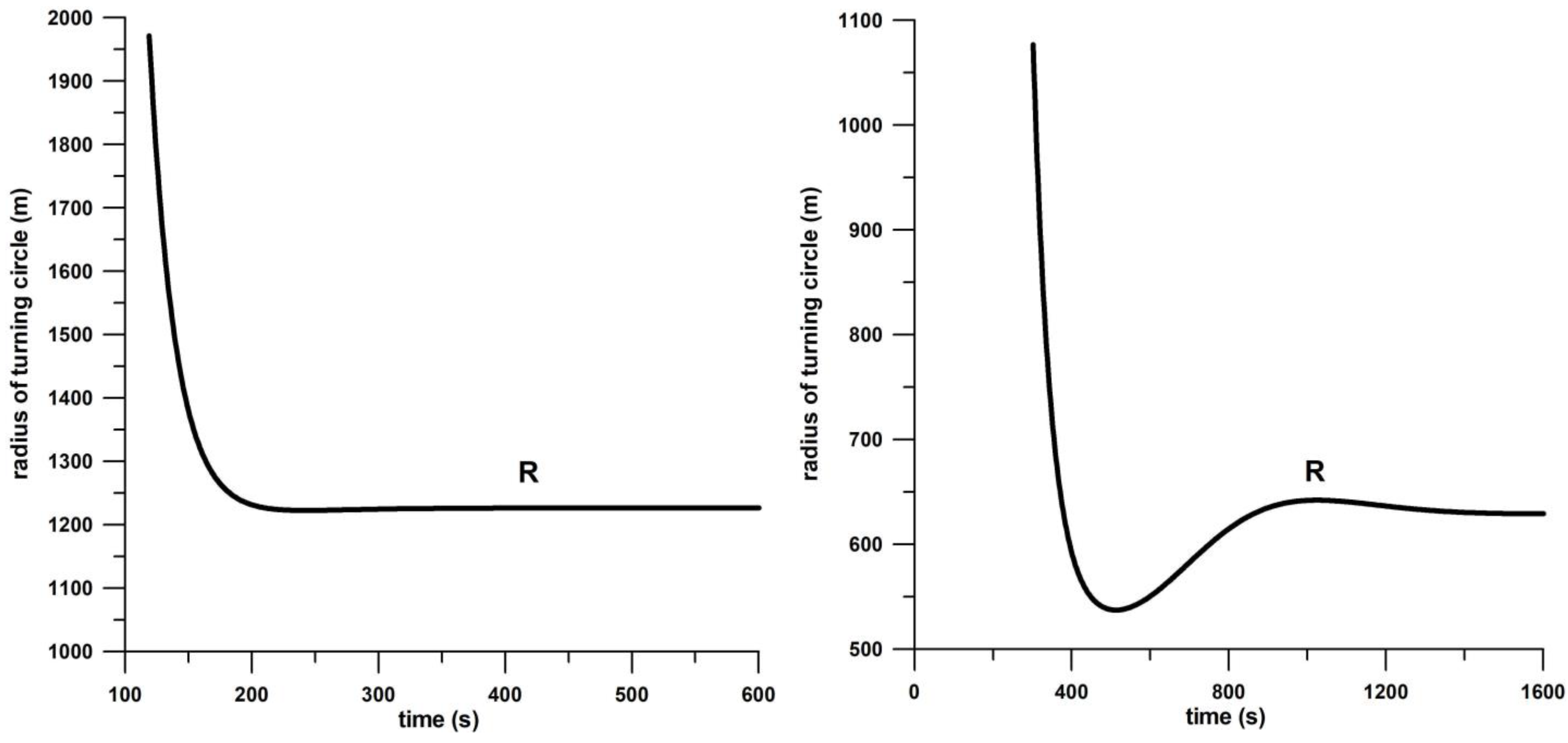
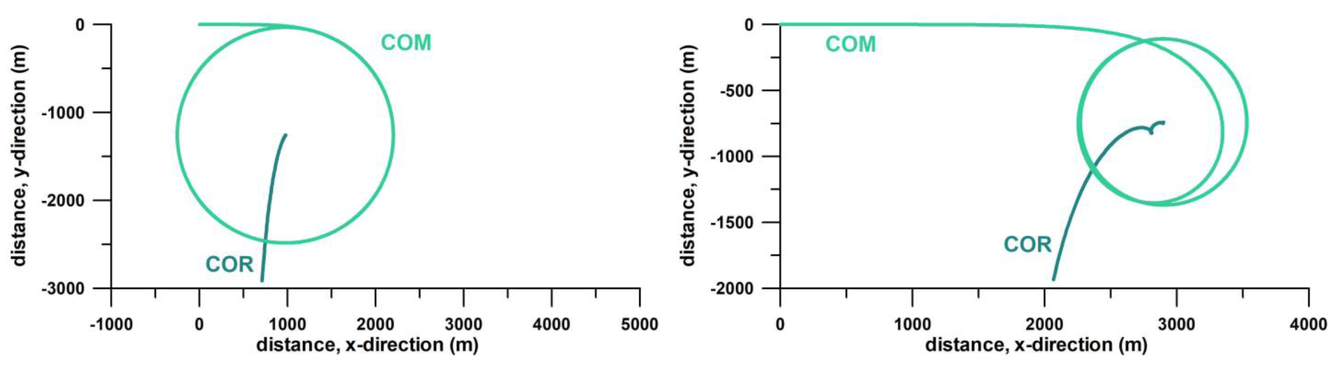
3.1.2. Turning Circle and Angle of Attack

Long and short radii R of the turning circles (Figure 9) are associated with flat and steep angles of attack AoA (Figure 10), respectively. Both R and AoA show significant under- and overshoots at the end of the transient phase of condition 2, a feature already seen in the velocity and acceleration graphs (Figure 5, Figure 6, Figure 7 and Figure 8). The movement of the centre of mass COM of the ship is shown in Figure 11, together with the centrode, that is, the curve of the centre of rotation COR. During the transient phase of condition 2, the trajectory of the COM intersects with the (future) turning circle in the steady state because of a transient increasing curvature (inverse of R; undershoot in Figure 9 (right) associated with a greater AoA (spike in Figure 10 (right)). The centrode approaches the centre of the turning circle from infinity, with a flatter gradient in condition 2, resulting from a greater ‘advance’ of the ship. Although short R and steep AoA are a feature of condition 2, the ’advance’ is not. This issue is addressed in the Discussion section.

Figure 9. Radius R of the turning circle versus time, for conditions 1 (left) and 2 (right).

Figure 9. Radius R of the turning circle versus time, for conditions 1 (left) and 2 (right).

Figure 10. Angle of attack AoA of the turning circle versus time, for conditions 1 (left) and 2 (right).

Figure 10. Angle of attack AoA of the turning circle versus time, for conditions 1 (left) and 2 (right).

Figure 11. Trajectory of the centre of mass COM, and centrode of the centre of rotation COR, for conditions 1 (left) and 2 (right).

Figure 11. Trajectory of the centre of mass COM, and centrode of the centre of rotation COR, for conditions 1 (left) and 2 (right).

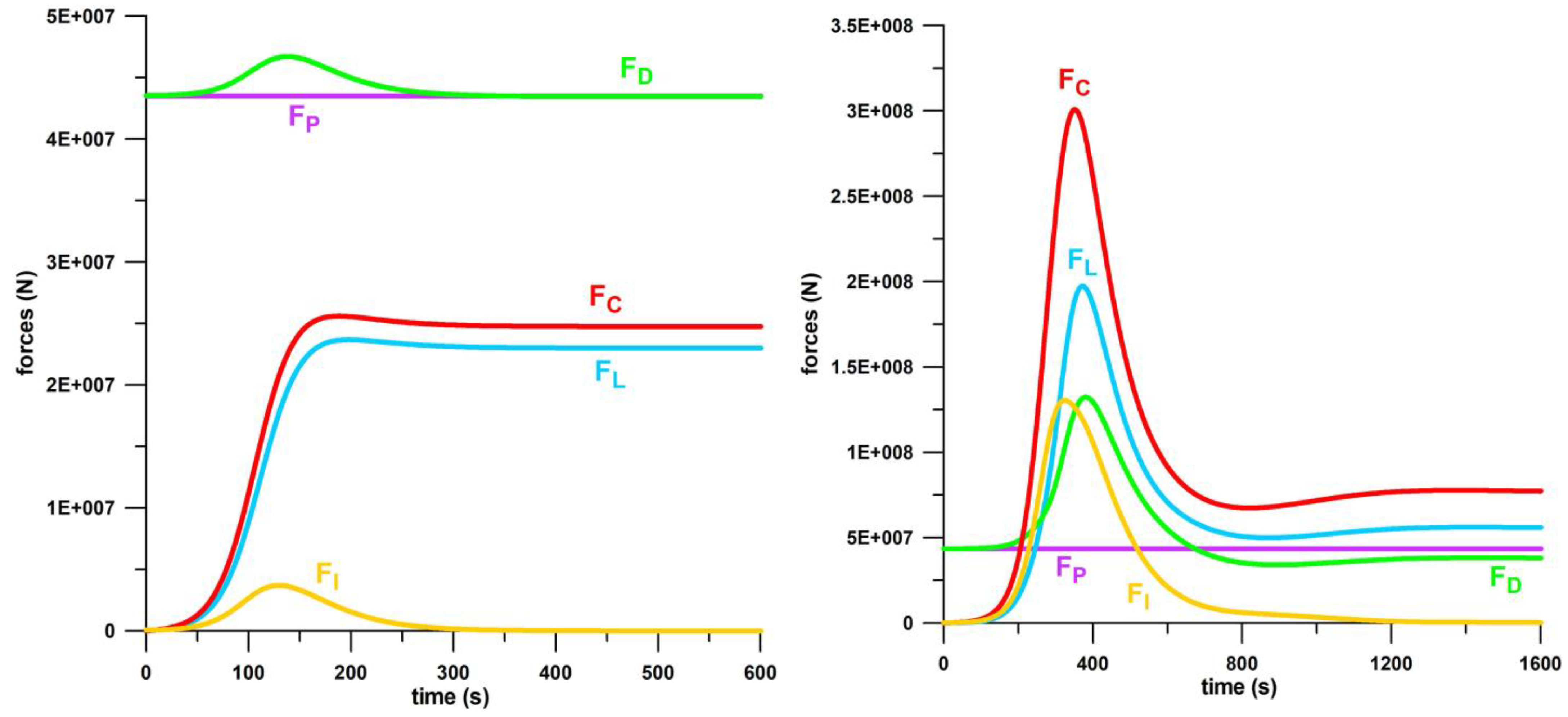
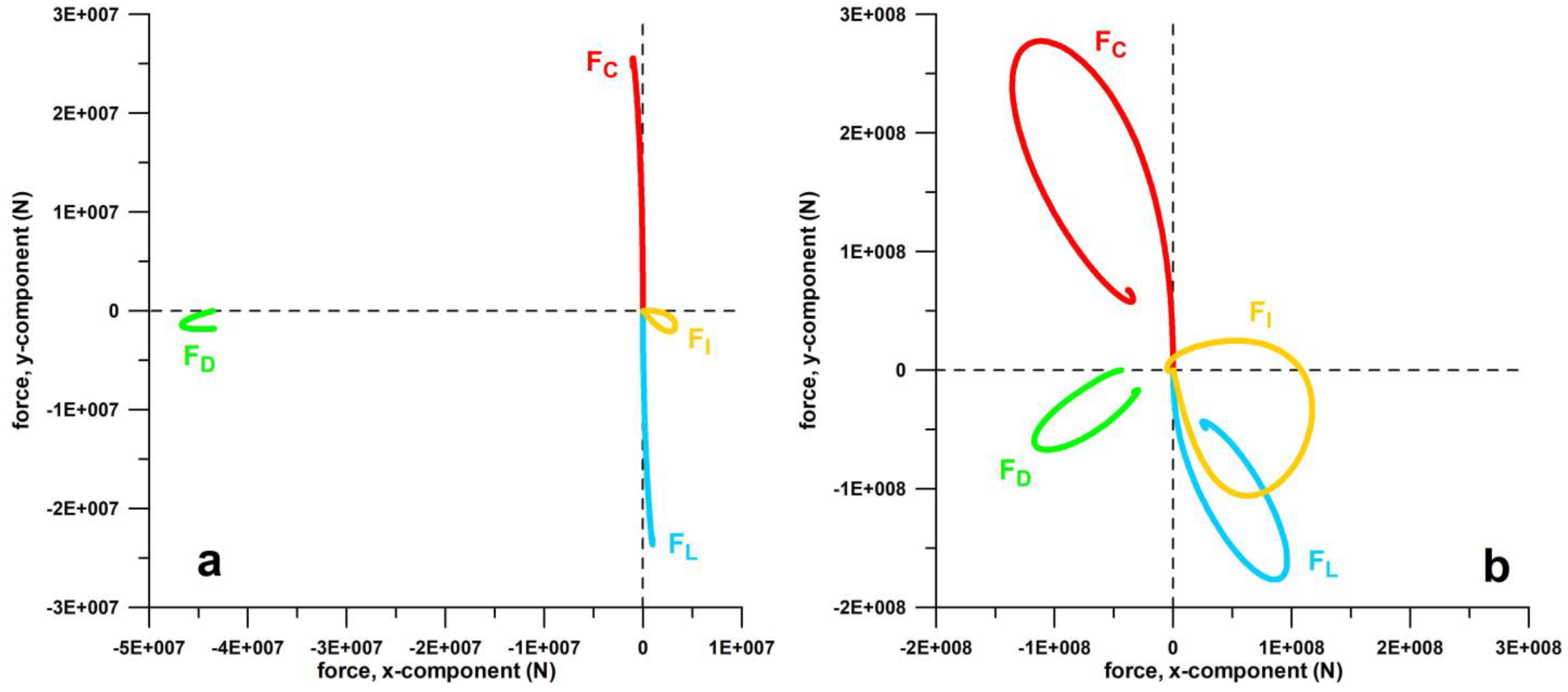
3.1.3. Forces and Their Vector Diagrams

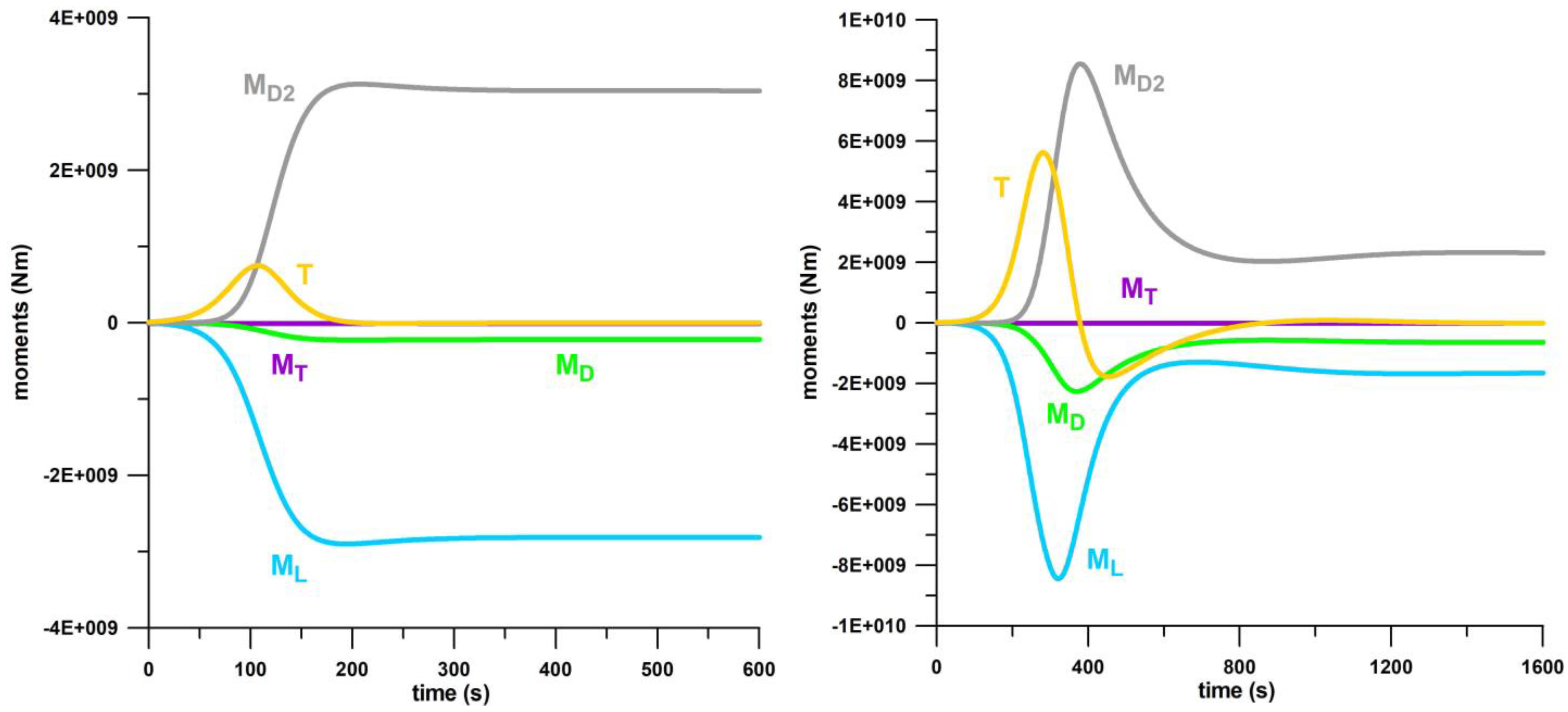
In condition 1, the forces are dominated by the drag force F_D, while in condition 2, they are dominated by the lift and centrifugal forces, F_L and F_C (Figure 12). The spikes of F_L and F_C are associated with the corresponding spikes of the AoA (Figure 10) and ω (Figure 7), respectively. The inertial force returns to zero, as the steady state is characterised by zero acceleration. The vector diagrams in Figure 13 show how the force vectors move with respect to the ship (reduced to a point at the origin of the coordinate system) during the transient phase. Figure 13a,b displays the envelopes of the vector diagrams (curve through the endpoints of the vectors) in conditions 1 and 2. While F_D and F_I are hook- and loop-shaped in both conditions, F_L and F_C are nearly straight in condition 1 and open-loop in condition 2. Both F_L and F_C form hooklets when they reach steady state. Figure 13 also reflects the size difference between F_D and F_I shown in Figure 12 (left) and Figure 13a, as well as the similar magnitudes of F_D and F_I displayed in Figure 12 (right) and Figure 13b. Figure 13c explains that the hook/loop envelopes can be broken down into two phases separated by the peak of a_x (Figure 6 (right)), which is roughly midway through the transient phase at the crests of the hooks/loops. Figure 13d shows the actual vectors associated with the envelopes. Throughout the turning motion, F_L and F_C point in opposite directions and are perpendicular to the velocity vector v and to the tangent at any point on the COM’s trajectory. F_C tends to push the ship outward while F_L tends to pull the ship into the turning circle. This equilibrium, even if F_L and F_C are not precisely of the same magnitude, is critical to maintaining a consistent trajectory on the turning circle. Two more components are required for this equilibrium, namely the F_P- and F_T-components perpendicular to vector v.

Figure 12. Forces versus time, for conditions 1 (left) and 2 (right); F_I: inertial force, F_C: centrifugal force, F_D: drag force, F_L: lift force, F_P: propulsive force. The sideward thruster force F_T is not included because it is comparatively very small.

Figure 12. Forces versus time, for conditions 1 (left) and 2 (right); F_I: inertial force, F_C: centrifugal force, F_D: drag force, F_L: lift force, F_P: propulsive force. The sideward thruster force F_T is not included because it is comparatively very small.

Figure 13. Vector diagrams, y-components versus x-components, with the ship reduced to a point mass; (a) conditions 1, envelope curves, connecting the tips of the vectors; (b) condition 2, envelope curves; (c) condition 2, envelope curve of vectors before and after the a_x-peak (identified by small arrows; cf. Figure 6(right)); (d) same as (c) plus actual force vectors; F_I: inertial force, F_C: centrifugal force, F_D: drag force, F_L: lift force.

Figure 13. Vector diagrams, y-components versus x-components, with the ship reduced to a point mass; (a) conditions 1, envelope curves, connecting the tips of the vectors; (b) condition 2, envelope curves; (c) condition 2, envelope curve of vectors before and after the a_x-peak (identified by small arrows; cf. Figure 6(right)); (d) same as (c) plus actual force vectors; F_I: inertial force, F_C: centrifugal force, F_D: drag force, F_L: lift force.

3.1.4. Moments

In Figure 14, condition 2 shows the already known spikes and undershoots (free moment T = α I) in the transient phase. The most important moments acting on the ship about its COM are the moment of the lift force M_L and the moment of the hydrodynamic force couple M_D2 (Figure 4). The lift force moment is essentially the moment of the force couple generated by the lift force and the centrifugal force (note that F_L and F_C do not have exactly the same magnitude).

Figure 14. Moments versus time, for conditions 1 (left) and 2 (right); T: free moment (= Iα), M_T: thruster moment, M_D: moment of drag force, M_L: moment of lift force, M_D2: moment of hydrodynamic force couple.

Figure 14. Moments versus time, for conditions 1 (left) and 2 (right); T: free moment (= Iα), M_T: thruster moment, M_D: moment of drag force, M_L: moment of lift force, M_D2: moment of hydrodynamic force couple.

3.2. Model Validation with Experimental Data

The turning radius calculated from the ship data provided by Gug et al. [29] was 179.7 m (Figure 15); the corresponding angle of attack AoA at steady state that resulted from the simulation was 4.07° (Figure 15). Despite the use of flat plate C_D, C_L, and COP data, the calculated turning radius R correlated well with the average radius of the turning circles (163.28 m and 183.56 m) experimentally determined from GPS data by Gug et al. [29] (p. 10, Table 7).

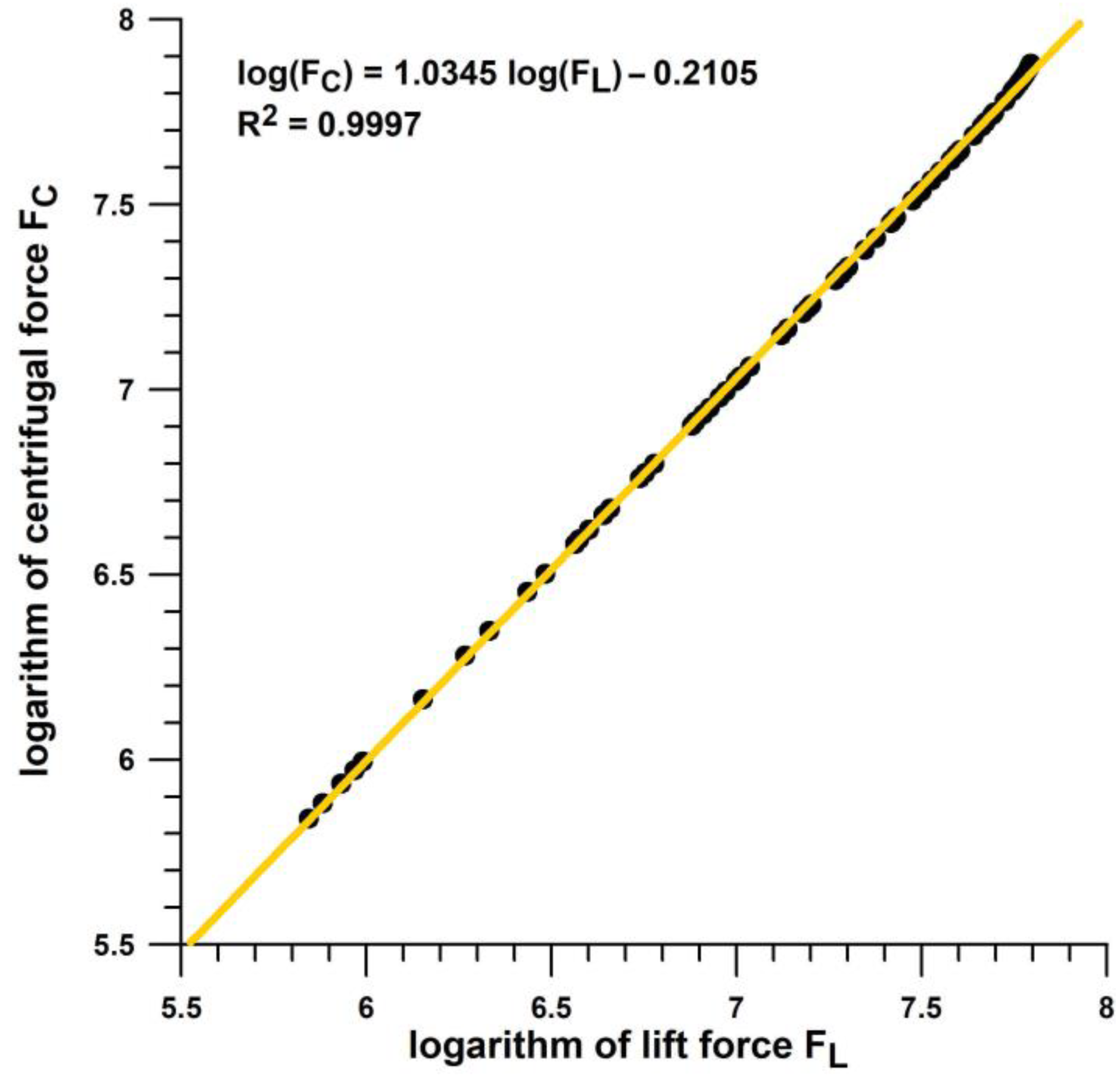
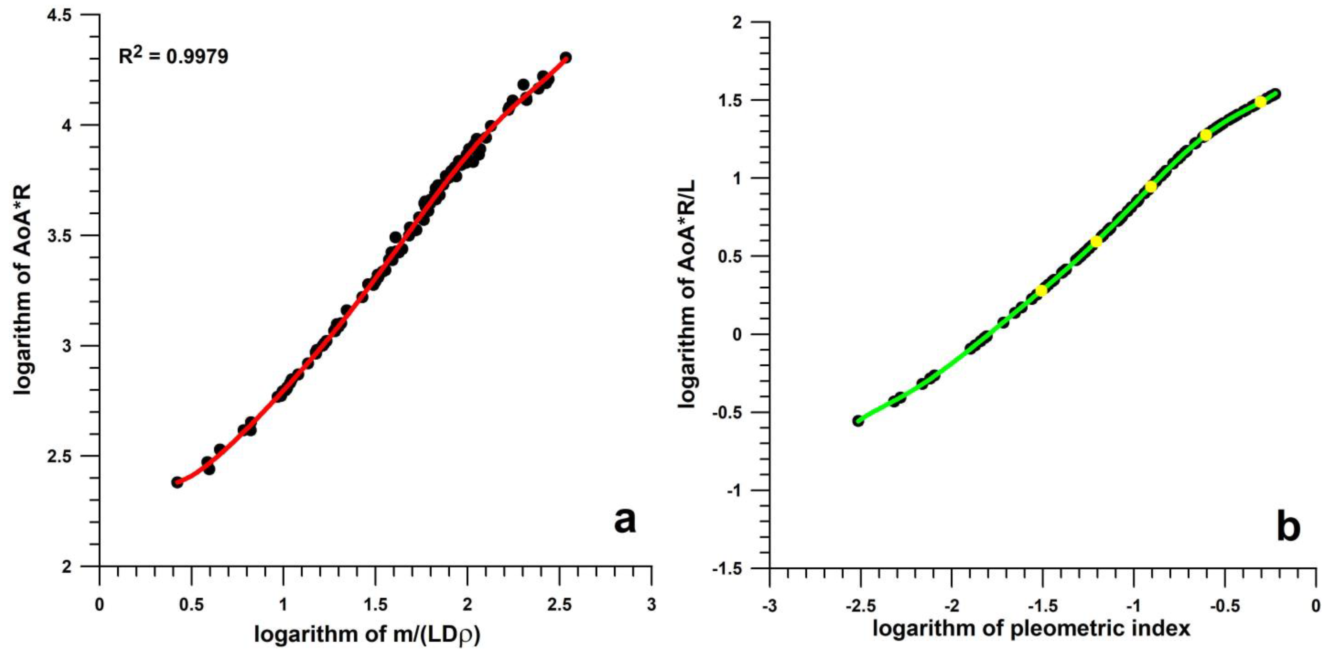
3.3. Proportionality of Lift and Centrifugal Forces, and Proposal of a Pleometric Index

As mentioned above, F_L and F_C, pulling the ship in and out of the turning circle, are critical to maintaining a consistent trajectory on the turning circle. Since they are not precisely the same magnitude, it has to be examined whether they are at least proportional in the steady state. With a proportionality constant of log(F_C)/log(F_L) between 1 and 1.011 (1.005 ± 0.003; Figure 16), we propose that

$$\log F_C \propto \mathrm{l}\mathrm{o}\mathrm{g}{F}_L$$

(26)

where log denotes the decadic logarithm.

Substituting Equations (5) and (7) into Equation (26) yields

$$-0.3+\log \rho +\log C_L+\log A+2\log v\propto \log m+\log R+2\log \omega$$

(27)

Substituting the log-transformed Equation (8) into the left-hand side of Equation (27) yields

$$-0.3+\log \rho +\log C_L+\log A+2\log R+2\log \omega \propto \log m+\log R+2\log \omega$$

(28)

After rearranging Equation (28), removing the constant of –0.3, and replacing C_L with the AoA (since C_L is an almost-linear function of AoA, up to an AoA of 30°; cf. Equation (2) and Figure 3), we obtain

$$\log \mathrm{A}\mathrm{o}\mathrm{A}+\log R \propto \log m-\log A-\log \rho$$

(29)

The right-hand side of Equation (29), in antilogarithmic form of

$$\frac{m}{A \rho }=\frac{m}{L D \rho }$$

(30)

but best expressed in the logarithmic form of Equation (29), explains the turning dynamics from the physical data of the ship or input data of the model. Increasing the mass m has the same dynamic effect as reducing any of the three parameters in the denominator of Equation (30), that is, length L, draught D, or water density ρ. Equation (29) becomes in antilogarithmic form:

$$\mathrm{A}\mathrm{o}\mathrm{A} R=\frac{m}{L D \rho }$$

(31)

The disadvantage of Equation (31) is that the unit of both sides is metres. In addition, if D is divided by 4 or 2, ρ by 4 or 2, and L by 2 or 1.414 (Table 1), the AoA remains the same, but R is double or 1.414 times longer in the D-variation than in the L-variation. To counteract this effect, we divide R by L (Table 1) so that when D is divided by 4 or L by 2, R/L becomes invariant. To maintain the integrity of Equation (31), we need to divide the right-hand side of Equation (31) by L as well, so that Equation (31) becomes dimensionless:

$$\mathrm{A}\mathrm{o}\mathrm{A} \frac{R}{L}=\frac{m}{L^2 D \rho }$$

(32)

The right-hand side of Equation (32) constitutes the decisive pleometric index 𐊬

$$\mathrm{𐊬}=\frac{m}{L^2 D \rho }$$

(33)

(from ancient Greek πλοῖον/ploîon, ‘ship, floating vessel’, and μετρεῖν/metreîn, ‘to measure’, where 𐊬 is the ancient form of the Greek letter Π) that characterises the dynamics of a turning ship. This pleometric index is proportional to the output parameters of the model, namely the AoA (related to the C_L of F_L, since C_L is a function of AoA according to Equation (2)) and the turning radius R (from F_C, Equation (7)), specially normalized to L, that is, R/L. These output parameters are crucial for describing the turning motion of a ship in the steady state. Increasing the mass m also increases the product of AoA and R/L, or the sum of logAoA and log(R/L).

Having established the relationship between F_C and F_L in Figure 16, the correlations between the various components of the pleometric index are shown in Figure 17. Using Figure 17b–d, the following parameters can be determined with a high accuracy from the pleometric index: log(AoA·R/L), logAoA, log(R/L).

4. Discussion

Based on the knowledge gap that emerged from the literature review, noting that free body diagrams (FBD) are uncommon and at best incomplete in ship dynamics research, the contribution to the literature provided by this study is the FBD approach to understanding the dynamics of a turning ship.

The novelty of this study is that it:

-

describes the changing dynamic variables (velocities, accelerations, turning radius, angle of attack, forces, moments) as a time series;

-

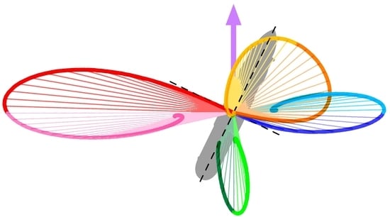
provides continuous vector diagrams of centrifugal, inertial, lift, and drag forces throughout the turning motion;

-

identifies the force couple of centrifugal and lift forces as the main source of stable equilibrium during the turn;

-

establishes the proportionality of centrifugal and lift forces;

-

derives from this proportionality a pleometric index 𐊬 for predicting the turning dynamics of a ship; and

-

calculates this pleometric index solely from the characteristics of a ship, namely as a function of its mass, length, and draught (and also the water density).

In this study it was shown that the dynamics of a turning ship can be predicted from the equations of forces and moments alone, obtained from the FBD.

The pleometric index 𐊬 is proportional to the product of the angle of attack AoA and the turning radius R normalized to the ship’s length L (i.e., R/L), the two most important parameters that characterise a steady turn. The angle of attack AoA increases as the turning radius R decreases (Figure 17d and Figure 18), resulting in an increase of the pleometric index 𐊬. 𐊬 is directly proportional to AoA and inversely proportional to R (Figure 17c). AoA is inversely proportional to R, but the influence of AoA on 𐊬 outweighs the influence of R. The pleometric index 𐊬 is calculated only from the parameters of the ship (m, L, D) and from the water density (ρ).

Halpern [24] (p. 7) suggested a different relationship between AoA and R/L, namely AoA ≈ 18 L/R. This equation implies that AoA·R/L ≈ 18, the function of which is shown in Figure 17d as log(R/L) = log18 − logAoA. Halpern’s equation [24] only applies to ships with a pleometric index 𐊬 of approximately 0.25, with a turning radius of 1.6 L and an AoA of 12°. In comparison, the calculated 𐊬 for the Seawise Giant [28] is 0.124, for the Korean training ship [29] 0.098, and for the Titanic (properties from [30]) 0.072. Figure 17b shows that the logarithm of AoA·R/L ranges from –0.5 to 1.5, which corresponds to AoA· R/L of 0.32–32. Hence AoA· R/L is not a constant (≈18) as suggested by Halpern [24].

Figure 18. Two clockwise turning ships with longer and shorter radii of the turning circles (2.37 and 1.42 ship lengths), smaller and larger angles of attack (3.3° and 21.3°, respectively), and different pleometric indices 𐊬(0.11 and 0.47, respectively); green semicircles: turning circles; orange bold line: ship’s position relative to the turning circle; blue horizontal lines: tangents to the turning circles at the position of the ship’s centre of mass.

Figure 18. Two clockwise turning ships with longer and shorter radii of the turning circles (2.37 and 1.42 ship lengths), smaller and larger angles of attack (3.3° and 21.3°, respectively), and different pleometric indices 𐊬(0.11 and 0.47, respectively); green semicircles: turning circles; orange bold line: ship’s position relative to the turning circle; blue horizontal lines: tangents to the turning circles at the position of the ship’s centre of mass.

The pleometric index is only applicable to the steady state with constant R, AoA, v and ω, where the following five forces are in equilibrium: F_P, F_T, F_C, F_D, and F_L (Figure 1b, Figure 12). During the transient phase, from the start of the turn to steady state, a sixth force contributes to the equilibrium, namely the inertial force F_I (Figure 1a and Figure 12), as the translational velocity v decreases (deceleration). The same principle applies to the equilibrium of the following four moments in the steady state: M_T, M_D, M_L, and M_D2 (Figure 14). In the transient phase, a fifth moment contributes to the equilibrium, the free moment T (Figure 14), due to the angular acceleration α of the ship.

The force vectors F_C, F_D, and F_L, and F_I continuously change their direction with respect to the ship during the transient phase as shown in Figure 13d, while the directions of F_P and F_T remain constant. The main difference in the force vector diagram and the force equilibrium between low and high pleometric indices 𐊬 (conditions 1 and 2; Table 2; Figure 13a,b) is that in condition 2, the envelopes of the force vectors produce pronounced hooks in F_C and F_L that follow the a_x-peak (Figure 13c) and correspond to the pronounced overshoot of F_C and F_L (Figure 12, right subfigure; Table 2). The peak of these overshooting forces coincides with the a_x-peak (Figure 13c).

From the point of view of concurrent force and moment equilibria, it is the force couple of lift, F_T, and centrifugal, F_C, forces, and the moment resulting from this force couple that keeps the turning ship in a stable equilibrium during the steady state. When calculating the moments about the ship’s centre of mass, then the moment of the lift force, M_L, and the moment from the water angularly displaced by the turning ship (Figure 4c), M_D2, are in equilibrium, keeping the turning ship in a stable equilibrium during the steady state.

Table 2 summarises the dynamic differences of ships with low and high pleometric indices 𐊬.

Table 2. Summary of the dynamic behaviour of parameters; L: length; D: draught; m: mass; ρ: density of fluid medium; 𐊬: pleometric index from Equation (33); ↓: low; ↑: high.

Parameter	Condition 1 (m↓, L↑, D↑, ρ↑, 𐊬↓)	Condition 2 (m↑, L↓, D↓, ρ↓ 𐊬↑)
turning radius R	longer	shorter, undershooting/oscillating before reaching the steady state
angle of attack AoA	lower/flatter	higher/steeper, overshooting/oscillating before reaching the steady state
translational velocity v, x- and y-components	vx >> vy	vx (undershooting) > vy (overshooting); vy can be temporarily greater than vx in the transient phase
translational acceleration a	smaller	greater (ay undershooting after spike)
angular velocity ω	smaller	greater (overshooting spike)
angular acceleration α	spike before steady state	undershooting after spike
forces	FC, FL < FD, FP	FC, FL > FD, FP; pronounced overshoot of FC and FL
envelopes of force vector diagrams	almost straight envelopes of FC and FL	envelopes with pronounced hooks of FC and FL
moments	smooth transition to steady state MD, ML, MD2	spikes of MD, ML, MD2 before the steady state; T undershooting after spike

Table 2. Summary of the dynamic behaviour of parameters; L: length; D: draught; m: mass; ρ: density of fluid medium; 𐊬: pleometric index from Equation (33); ↓: low; ↑: high.

Parameter	Condition 1 (m↓, L↑, D↑, ρ↑, 𐊬↓)	Condition 2 (m↑, L↓, D↓, ρ↓ 𐊬↑)
turning radius R	longer	shorter, undershooting/oscillating before reaching the steady state
angle of attack AoA	lower/flatter	higher/steeper, overshooting/oscillating before reaching the steady state
translational velocity v, x- and y-components	vx >> vy	vx (undershooting) > vy (overshooting); vy can be temporarily greater than vx in the transient phase
translational acceleration a	smaller	greater (ay undershooting after spike)
angular velocity ω	smaller	greater (overshooting spike)
angular acceleration α	spike before steady state	undershooting after spike
forces	FC, FL < FD, FP	FC, FL > FD, FP; pronounced overshoot of FC and FL
envelopes of force vector diagrams	almost straight envelopes of FC and FL	envelopes with pronounced hooks of FC and FL
moments	smooth transition to steady state MD, ML, MD2	spikes of MD, ML, MD2 before the steady state; T undershooting after spike

The pleometric index 𐊬 should not be confused with the controllability of a ship. The term ‘controllability’ in this context refers to how quickly and how extensively a ship reacts when initiating a turn. This response can be expressed by the amount of rotation or lateral movement in y-direction within a given timeframe or after a defined movement in x-direction (Figure 19). A more responsive ship with better controllability will move further within a certain time or movement (x-direction) window. The parameter responsible for the controllability is the moment of inertia I, the product of mass and radius of gyration squared. For a slender rod, rotating about its centre, I = m L²/12. In contrast, the pleometric index depends on the ratio of m to L² (Equation (33)), but not on their product (m L²).

The underlying hydrodynamic principle of the ship was modelled as a flat plate for several reasons:

• The hydrodynamic equations used by Reference [19] apply the lateral area of a ship as the reference surface for hydrodynamic calculations (mean draught times ship length), which is the standard for streamlined bodies such as symmetrical aerofoils, cambered aerofoils, flat plates with AoAs smaller than the stall angle, and teardrop shapes without or with Kamm tails.
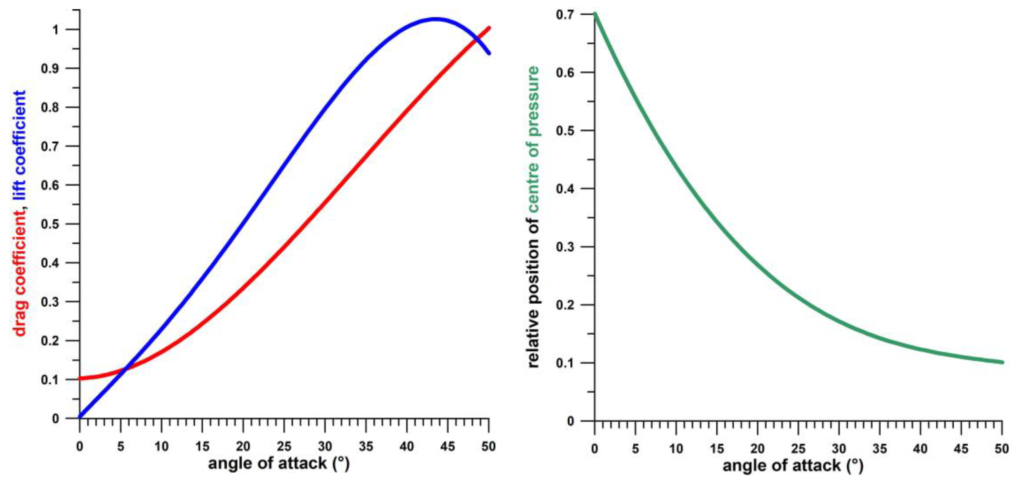
• Fluid dynamic data of flat plates at extreme aspect ratios are available in the literature [27], in particular on drag and lift coefficients, and the position of the fluid dynamic centre of pressure (COP), all expressed as a function of the angle of attack. In order to run the model under realistic conditions, these input data are taken from flat plates [27].
• Larger vessels such as oversized containerships and oil tankers have a constant width (beam) over most of the ship’s length, and therefore resemble flat plates rather than symmetrical aerofoils. Other ships do not have a constant width and so do not resemble flat plates, but still resemble symmetrical streamlined bodies, so the general principles of drag, lift, and COP apply at different AoA—specifically that the drag coefficient increases as the AoA does; the lift coefficient increases up to a certain stall angle and then decreases as the AoA further increases; and the COP moves from the front stagnation point closer to the centroid of the streamlined body as the AoA increases.

To compare the validity of the model to experimental data, the ship characteristics of Gug et al. [29] were used as input for the simulation. The turning radius R of 179.7 m as the model output (Figure 15) was of comparable magnitude to the turning circle radius (163.28 m and 183.56 m, port and starboard, respectively) experimentally determined from GPS data by Gug et al. [29]. This result suggests that the flat plate model is applicable to the training ship used by Gug et al. [29].

One of the advantages of using the FBD approach is that the forces’ equations allow the immediate identification of unknown parameters required for modelling and simulations (item 6 under the list of purposes of FBDs at the beginning of the Introduction section). Once the unknown parameters are identified, tests to experimentally determine these parameters can be planned. These experiments, to be conducted with ship models of different hull, draught, and length geometry, are devised as follows:

(1)

Drag and lift experiments at realistic Reynolds numbers and at different AoAs. The models were to be statically mounted on a 6-DOF force and moment transducer in a water tunnel. These experiments serve to determine the drag and lift coefficients, as well as the COP as functions of AoA.

(2)

Dynamic measurement of water resistance as the ship model rotates about its COM in a water tank. A 1-DOF moment transducer should be placed between the rotation axis and the hull of the model to measure the free moment of the hydrodynamic force couple and determine the drag coefficient of the free moment.

(3)

Combination of (1) and (2) by rotating the model, rigidly and eccentrically mounted to a rotating axle with its COM offset from the axle in a water tank. The offset (i.e., the turning radius R) as well as the AoA should be adjustable. Since the combination of the chosen parameters of R, AoA, angular velocity ω, and mass m does not necessarily lead to a force and moment equilibrium of the model, further reaction-forces and -moments are generated at the interface between model and axle, which are measured by a 6-DOF force and moment transducer. Based on the measured forces and moments, the unknown drag and lift forces and their moments including the free moment of the hydrodynamic force couple can be calculated. The calculated parameters serve to validate the hydrodynamic parameters obtained from (1) and (2).

Reference [19] offers four different tests to be performed in a towing tank to determine the hydrodynamic parameters. The static drift test at a constant drift angle (AoA) allows direct measurement of drag and lift forces, and calculation of the drag and lift coefficients.

Another benefit of FBDs is that the equilibrium of forces can directly lead to dynamic indices. A typical example is the FBD of a skier gliding downhill [31] (pp. 2–3, Figure 1D). When gliding at the terminal velocity, the drag force and the force component of the gravitational force parallel to the slope are in equilibrium (steady state, constant velocity, zero acceleration). The constants involved in this force equilibrium are the gravitational acceleration g, the mass m of the skier plus equipment, and the drag area Ad (product of frontal area and drag coefficient). The terminal velocity is proportional to the square root of the ratio of m·g to Ad [31,32] (p. 4). This square root has been termed the ‘anthropometric code number’ [32] (pp. 349–350), which explains why heavier and smaller skiers are faster.

By analogy, the proportionality of lift and centrifugal forces, F_L and F_C, shown in the FBD in Figure 1b and verified in Figure 16, resulted in an index that in this study is proposed to be called the pleometric index. This index, 𐊬, presented in Equation (33), is proportional to the product of AoA and R, divided by L. In addition, this index depends on the ship’s hull geometry, as the coefficient of lift varies with both the AoA and the hull geometry.

According to the ABS [22] (p. 68), ‘The force on the rudder is usually small in comparison to forces on the hull, so the rudder is only the initiator of a turn, while the hull lift force actually makes the vessel turn. The hull works as a lifting surface with a very small ratio between chord and span’. This statement is clearly reflected in Figure 14 and shows that the greatest turning moment is generated by the lift force (opposed by the moment of the hydrodynamic force couple, M_D2), while the moment of the thruster force, M_T, is negligible.

Witkowska et al. [33] simulated a ship’s turning circle under ballast and full load conditions, and their results show a shorter R and less ‘advance’ under full load. This result is only partially reflected in the results of the present study. While Figure 11 (condition 2) reflects a shorter R under greater mass, the advance is longer. The parameters of conditions 1 and 2 are not necessarily directly related to the magnitude of a ship’s advance. If the initial translational velocity is the same for all conditions, then the advance depends on the turning ability of a ship. The ability to turn is characterized by the moment of inertia as explained in Equation (23): for the same turning moment T, a ship with more I accelerates less angularly. I increases as the mass and/or the length does. Therefore, an increase in mass m takes a longer time to turn the ship with a longer advance, whereas a shorter length L turns the ship faster with a shorter advance. Both conditions (more mass, shorter length) define condition 2 and result in a shorter radius R. It is therefore expected that the results of Witkowska et al. [33] show a longer advance rather than a shorter one.

Benedict [25] plots the path of turning ship and in his (incomplete) FBD includes only lateral forces, perpendicular to the ship’s longitudinal (or roll) axis. These forces are: Y(δ)—rudder force (1:00 min in the video), Y(β)—(hydrodynamic) lift force (at 2:50 min.), Y_Centrifugal—centrifugal force (at 3:50 min), and Y(r)—referred to as ‘so-called damping force’ (at 4:00 min). The ship’s angle of attack AoA is referred to as angle β. Benedict’s [25] FBD is affected by some mistakes.

Benedict [25] compares the hull of the ship to an aerofoil and claims that Y(β) would be a lift force. However, Y(β) is neither perpendicular to the ship’s velocity vector nor to the free airstream acting on the aerofoil in the lower right inset of the video. By definition, the drag force acts against the free airstream and in opposition to the velocity vector of a vehicle or aerofoil, while the lift force acts perpendicular to these vectors. Benedict’s [24] lift force could be the resultant force of drag and lift forces, but this resultant is not necessarily perpendicular to the longitudinal axis of the ship.

By definition, the centrifugal force is collinear with the line connecting COR and COM. The centrifugal force originates from the COM and points away from the COR. Therefore, the centrifugal force is perpendicular to the translational velocity vector of the COM. In Benedict’s [25] FBD, the centrifugal force is perpendicular to the ship’s longitudinal axis, even though the COM’s translational velocity vector is inclined at an angle of attack (AoA, β) greater than zero.

Benedict [25] did not explain where the single force vector Y(r), the ‘so-called damping force’ comes from. He explains that the moment of Y(r) is in equilibrium with moments of Y(δ) and Y(β), the moments apparently being taken about the COM, since Y_Centrifugal, originating from the COM, generates no moment. Therefore, the alleged damping force is an eccentric force, which excludes force couples. A damping force is commonly referred to as a force that slows or stops a motion. Therefore, the damping force is an applied force, originating from a centre of pressure, that dissipates energy, such as drag and friction forces (surface friction or viscous friction). The only motion that is dampened at the transition from the transient phase to the steady state is the oscillation of the acceleration around the zero line. Figure 20, a double logarithmic display of Figure 8, shows these oscillations, where the angular acceleration of condition 1 oscillates only once and is then critically damped, whereas the angular acceleration of condition 2 is underdamped and continues to oscillate. However, the origin or cause of Benedict’s [25] damping force is unknown. In theory, the hydrodynamic force couple (Figure 4) with its moment M_D2 (Figure 14) is a likely candidate for performing this damping action—simply because it is of similar magnitude and pattern to the moment of the lift force, M_L. Exactly this moment counteracts Benedict’s [25] mysterious damping force Y(r). If one only reduces the magnitude of the moment M_D2, then the angular acceleration of condition 1 is no longer critical, but underdamped (Figure 21), and behaves like the angular acceleration of condition 1 (Figure 20). This result suggests that Benedict’s [25] damping force Y(r) is more the hydrodynamic force couple illustrated in Figure 4 than like a single eccentric force. In addition, reducing the magnitude of the moment M_D2 generally has the same effect as condition 2 has (great m, short L and D, and low ρ).

5. Conclusions

Based on the literature review presented in the introductory section, it is both surprising and unexpected that a classic dynamic example of a turning ship is utterly lacking in the correct application of free body diagrams, which are incomplete at best and often flawed.

The free body diagram approach used in this study led to specific novelties in the field of ship dynamics, such as the inclusion of all forces and moments acting on a ship in the transient and steady state phases of a turn; presentation of the dynamic variables resulting from the model simulation (velocities, accelerations, turning radius, angle of attack, forces, moments) as a time series; visualisation of the continuous vector diagrams and their changing directions over time of centrifugal, inertial, lift and drag forces throughout the turning motion; identification of the force couple of centrifugal and lift forces as the main source of stable equilibrium during the turn; investigation of the proportionality of centrifugal and lift forces; derivation and thus proposal of a pleometric index 𐊬 for predicting the rotational dynamics of a ship; and calculating said pleometric index solely from the characteristics of a ship, as functions of mass, length, draught, and water density.

Ships that are heavier, shorter and shallower (and sail in fresh water) have a larger pleometric index and turn on a shorter-radius circle with a steeper angle of attack. In terms of dynamics, a larger pleometric index leads to increased fluctuations in velocities, accelerations, forces, and moments (Table 2). The pleometric index (m·L⁻²·D⁻¹·ρ⁻¹) is (1) nonlinearly proportional to the product of AoA and R/L with a positive gradient; (2) nonlinearly proportional to the AoA with a positive gradient; and (3) nonlinearly proportional to the R/L with a negative gradient. Likewise, AoA and R/L are nonlinearly proportional with a negative gradient, with the influence of the AoA on the pleometric index outweighing that of R/L.

References

1. Shames, I.H. Engineering Mechanics: Statics, 4th ed.; Prentice Hall: Hoboken, NJ, USA, 1997; p. 152. [Google Scholar]
2. Le Rond d’Alembert, J.-B. Traité de Dynamique; M.-A. David (David l’aîné): Paris, France, 1743. [Google Scholar]
3. Triantafyllou, M.S.; Hover, F.S. Maneuvering and Control of Marine Vehicles; MIT Press: Cambridge, MA, USA, 2003. [Google Scholar]
4. Lewandowski, E.M. The Dynamics of Marine Craft: Maneuvering and Seakeeping (Volume 22 of Advanced Series on Ocean Engineering); World Scientific: Singapore, 2004. [Google Scholar]
5. Newman, J.N. Marine Hydrodynamics; MIT Press: Cambridge, MA, USA, 2018. [Google Scholar]
6. Shuai, Y.; Li, G.; Xu, J.; Zhang, H. An Effective Ship Control Strategy for Collision-Free Maneuver Toward a Dock. IEEE Access 2020, 8, 110140–110152. [Google Scholar] [CrossRef]
7. Kijima, K.; Katsuno, T.; Nakiri, Y.; Furukawa, Y. On the manoeuvring performance of a ship with the parameter of loading condition. J. Soc. Nav. Archit. Jpn. 1990, 1990, 141–148. [Google Scholar] [CrossRef] [PubMed] [Green Version]
8. Perara, L.P. Ship maneuvring prediction under navigation vector multiplication based pivot point estimation. IFAC-Pap. OnLine 2015, 48, 1–6. [Google Scholar] [CrossRef]
9. Inoue, S.; Hirano, M.; Kijima, K. Hydrodynamic derivatives on ship manoeuvring. Int. Shipbuild. Prog. 1981, 28, 112–125. [Google Scholar] [CrossRef]
10. Yoshimura, Y. Mathematical model for the manoeuvring ship motion in shallow water. J. Kansai Soc. Nav. Archit. Jpn. 1986, 200, 41–51. (In Japanese) [Google Scholar]
11. Yoshimura, Y. Mathematical model for the manoeuvring ship motion in shallow water (2nd report). J. Kansai Soc. Nav. Archit. Jpn. 1988, 210, 77–84. (In Japanese) [Google Scholar]
12. Yoshimura, Y. Mathematical model for manoeuvring ship motion (MMG model). In Proceedings of the Workshop on Mathematical Models for Operations Involving Ship-Ship Interaction, Tokyo, Japan, 4–5 August 2005; pp. 1–6. [Google Scholar]
13. Pérez, F.L.; Clemente, J.A. The influence of some ship parameters on manoeuvrability studied at the design stage. Ocean Eng. 2007, 34, 518–525. [Google Scholar] [CrossRef]
14. Carreño Moreno, J.E.; Sierra Vanegas, E.Y.; Jiménez González, V.H. Ship maneuverability: Full-scale trials of Colombian Navy Riverine Support Patrol Vessel. Ship Sci. Technol. 2011, 5, 69–86. [Google Scholar] [CrossRef]
15. Carreño, J.E.; Mora, J.D.; Pérez, F.L. A study of shallow water’s effect on a ship’s pivot point. Ing. E Investig. 2012, 32, 27–31. [Google Scholar] [CrossRef]
16. Carreño, J.E.; Mora, J.D.; Pérez, F.L. Mathematical model for maneuverability of a riverine support patrol vessel with a pump-jet propulsion system. Ocean Eng. 2013, 63, 96–104. [Google Scholar] [CrossRef]
17. Liu, J. A Primer of Inland Vessel Maneuverability. In Mathematical Modeling of Inland Vessel Maneuverability Considering Rudder Hydrodynamics; Liu, J., Ed.; Springer: Cham, Switzerland, 2020; pp. 99–127. [Google Scholar] [CrossRef]
18. Huang, H.-R.; Wang, Y.-L. Simulation of ship maneuvering using the plane motion model. Indian J. Geo Mar. Sci. 2017, 46, 2250–2257. [Google Scholar]
19. ITTC (International Towing Tank Conference). ITTC—Recommended Procedures. Uncertainty Analysis for Manoeuvring Predictions Based on Captive Manoeuvring Tests; ITTC Association: Zürich, Switzerland, 2014. [Google Scholar]
20. Ji, Z.; Huang, Y. Autonomous boat dynamics: How far away is simulation from the high sea? In Proceedings of the OCEANS 2017, Aberdeen, Scotland, UK, 19–22 June 2017; pp. 1–8. [Google Scholar] [CrossRef] [Green Version]
21. Bowles, J. Turning characteristics and capabilities of high-speed monohulls. In Proceedings of the 3rd Chesapeake Power Boat Symposium, Annapolis, MD, USA, 15–16 June 2012; pp. 1–18. [Google Scholar]
22. ABS (American Bureau of Shipping). Guide for Vessel Maneuverability; ABS: Houston, TX, USA, 2017. [Google Scholar]
23. Cheirdaris, S. Lecture 2: Controlling Ship Dynamics; Aalto University: Espoo, Finland, 2021. [Google Scholar]
24. Halpern, S. She Turned Two Points in 37 Seconds. 2010. Available online: http://www.titanicology.com/Titanica/Two-Points-in-Thirty-Seven-Seconds.pdf (accessed on 5 June 2023).
25. Benedict, K. Theory behind Turning Dynamics of Ships. YouTube Video. 2020. Available online: https://www.youtube.com/watch?v=_qM8OjmrzPM (accessed on 28 March 2021).
26. Matusiak, J. Dynamics of a Rigid Ship; Aalto University Publication Series; Aalto University: Espoo, Finland, 2013. [Google Scholar]
27. Ortiz, X.; Rival, D.; Wood, D. Forces and moments on flat plates of small aspect ratio with application to PV wind loads and small wind turbine blades. Energies 2015, 8, 2438–2453. [Google Scholar] [CrossRef] [Green Version]
28. Seawise Giant. Available online: https://en.wikipedia.org/wiki/Seawise_Giant (accessed on 28 November 2022).
29. Gug, S.G.; Harshapriya, D.; Jeong, H.; Yun, J.H.; Kim, D.J.; Kim, Y.G. Analysis of manoeuvring characteristics through sea trials and simulations. The 3rd International Conference on Maritime Autonomous Surface Ship (ICMASS 2020). IOP Conf. Ser. Mater. Sci. Eng. 2020, 929, 012034. [Google Scholar] [CrossRef]
30. Titanic. Available online: https://en.wikipedia.org/wiki/Titanic (accessed on 7 June 2023).
31. Fuss, F.K. Slipstreaming in gravity powered sports: Application to racing strategy in ski cross. Front. Physiol. 2018, 9, 1032. [Google Scholar] [CrossRef] [PubMed]
32. Luethi, S.M.; Denoth, J. The influence of aerodynamic and anthropometric factors on speed in skiing. Intl. J. Sport Biomech. 1987, 3, 345–352. [Google Scholar] [CrossRef]
33. Witkowska, A.; Śmierzchalski, R.; Tomera, M.; Świsulski, D. Simulation of Ship Turning Circle Test for Ballast and Full Load Conditions [Dataset]; Gdańsk University of Technology: Gdańsk, Poland, 2020. [Google Scholar] [CrossRef]
Figure 4. Hydrodynamic forces acting on a turning ship; (a) ship turning in the steady state phase about a centre of pressure (COR), at a given angle of attack (AoA), and with a defined translational speed (v), angular velocity (ω), and turning radius (R); (b) translational component of the velocity (v) with the COR at infinity, resulting in drag (force FD) and lift (force FL); (c): rotational component of the velocity (ω) about the centre of mass (COM), resulting in varying pressure (p) differentials along the plate, between front and rear side; (d) equivalent force couple (FD2) resulting from integration of the pressure differential across the plate (FD2 vectors originating from centre of pressure COP2).
Dynamics 03 00021 g004
Figure 15. Trajectories of the centre of mass COM, and centrode of the centre of rotation COR, calculated from the ship dimensions of reference [29] (left); and angle of attack AoA versus the time (right).
Dynamics 03 00021 g015
Figure 16. Logarithm of centrifugal force FC versus logarithm of lift force FL; R2 = 0.9997, RSS = 0.0080 (data for: 0.03° < AoA < 19° at the steady state).
Dynamics 03 00021 g016
Figure 17. Correlation of input parameters (m, L, D, ρ), AoA and R; m: mass, L: length, D: draught, ρ: fluid density, R: radius of turning circle; AoA: angle of attack; (a) logarithm of the product of AoA and R versus the logarithm of m/(L·D·ρ), 7th order polynomial fit, R2 = 0.9979, RSS = 0.0461; (b) data of (a) normalized to L, pleometric index = m/(L2·D·ρ), 7th order polynomial fit, R2 > 0.9999, RSS = 0.0004, the 5 yellow dots represent the data of Table 1 (last 2 columns); (c) logarithm of AoA and of R/L versus the logarithm of the pleometric index, AoA fit: 6th order polynomial, R2 > 0.9999, RSS: 0.0020, R/L fit: 5th order polynomial, R2 > 0.9999, RSS: 0.0006; (d) logarithm of R/L versus the logarithm of AoA, 7th order polynomial fit, R2 > 0.9999, RSS = 0.0001; H = relationship between R/L and AoA proposed by Halpern [24] (cf. Discussion).
Dynamics 03 00021 g017aDynamics 03 00021 g017b
Figure 19. Motion in y-direction against time and motion in x-direction of three ships with different moments of inertia (MoI): 1 MoI (reference), 4 MoI and 0.25 MoI; the corresponding lateral movements (y-direction) after 16 s are: 0.3 m, 1.5 m, and 12 m; the lateral movements (y-direction) after 200 metres of advance in x-direction are: 3.7 m, 7.5 m and 12 m.
Dynamics 03 00021 g019
Figure 20. Angular acceleration of Figure 8ab versus time, in absolute values, with original positive (+α) and negative (–α) values shown in different colours.
Dynamics 03 00021 g020
Figure 21. Angular acceleration of Figure 8a versus time, in absolute values, with original positive (+α) and negative (–α) values in different colours, and the same acceleration resulting from reduced MD2 versus time.
Dynamics 03 00021 g021
Disclaimer/Publisher’s Note: The statements, opinions and data contained in all publications are solely those of the individual author(s) and contributor(s) and not of MDPI and/or the editor(s). MDPI and/or the editor(s) disclaim responsibility for any injury to people or property resulting from any ideas, methods, instructions or products referred to in the content.