1. Introduction
Quantum Field Theory (QFT) is a powerful tool to describe various phenomena in nature. It is applied in cosmology, elementary particle physics, nuclear physics, condensed matter physics, and biology. It can describe both microscopic degrees of freedom in Quantum Mechanics and macroscopic matter in Classical mechanics. (QFT is distinguished from Quantum mechanics, which can be applied only to the microscopic world). In particular, its application to the brain might be a promising approach in describing the mechanism of memory formation in the human brain [
1,
2].
Quantum Field Theory of the brain or Quantum Brain Dynamics (QBD) can be traced back to the monumental work by Ricciardi and Umezawa in 1967 [
3]. The brain is a mixed system of classical neurons and quantum degrees of freedom in QFT, namely corticons and exchange bosons [
4,
5]. The macroscopic vacua emerging in the spontaneous breakdown of symmetry (SBS) in QFT correspond to memory storage, and the creation of Nambu–Goldstone (NG) bosons emerging in SBS corresponds to memory retrieval. Since the vacua are maintained by long-range correlations by massless NG bosons, they describe non-local and stable features of memory. In 1968, Fröhlich suggested that the coherence with long-range correlation might occur in biological systems, resulting in boson condensation. As a result, the system with boson condensation operates as a single entity, called the Fröhlich condensate [
6,
7]. In 1976, Davydov and Kislukha proposed a model for a solitary wave propagation along protein
-helical structures, called the Davydov soliton [
8]. The Fröhlich condensate and the Davydov soliton emerge as mirror images of each other, namely as static and dynamical features in the nonlinear Schrödinger equation involving an equivalent Hamiltonian [
9]. Del Giudice et al. investigated quantum phenomena in biological systems in the 1980s [
10,
11,
12,
13]. In particular, they studied laser-like phenomena of water molecule rotational dipole fields and photon fields in [
12]. In the 1990s, Jibu and Yasue introduced concrete degrees of freedom in QBD, namely water dipole fields and photon fields [
1,
14,
15,
16,
17]. Vitiello suggested squeezed coherent states of Nambu–Goldstone bosons in dissipative QFT by regarding the brain as an open system [
18]. The diversity of memories is described by diverse squeezed coherent states which are unitarily inequivalent due to infinite degrees of freedom in QFT. Today, QBD remains as one of hypotheses expected to describe memory in the brain. Both single neurons and their groups generate differential electrostatic potentials in the extracellular matrix due to the electrical currents propagating in the form of action potentials. The generated electric field can be studied using extracellular electrodes [
19]. The brain’s EM waves were proposed to propagate within the cellular membrane in neuronal axons which, with electrolyte solution, form a “soft material wave guide” for electromagnetic (EM) signal transmission [
20]. Since the magnetic permeability of biological tissues is similar to that of a vacuum, the magnetic field is not distorted by scalp or skull. The source of magnetic fields is a dendritic current generated by over 50,000 pyramidal neurons that fire synchronously in parallel, while axonal and synaptic currents and magnetic fields largely cancel each other out. The amplitude of the brain’s magnetic fields is very insignificant, being smaller than pT [
21,
22]. Cerebrospinal Fluid (CSF), however, plays a major role in volume conductor models and current distribution, due to its relatively high electric conductivity [
23,
24]. In fact, CSF exhibits the highest value of electrical conductivity of all parts of the human body. Living organisms tend to be favorably affected by coherent patterns of EM waves, which may induce a “biological order” [
25].
Fröhlich’s theory of biological coherence is based on quantum interactions between dipoles of the polar head groups of cell membranes. The model requires the following pre-conditions to be satisfied: (a) A steady supply of energy above a minimum threshold level required for synchronization of membrane dipole oscillations, (b) The existence of a large trans-membrane potential difference. (c) Nonlinear interactions between the oscillating dipoles that generate a metastable non-equilibrium state. The resultant coherent state is due to the quantum condensation of dipolar vibrations. The supplied biochemical energy is channeled into a single strongly excited mode. Associated with this macroscopic quantum state is the emergence of electric polarization due to the ordering of dipoles. Fröhlich predicted the existence of coherent modes of dipolar excitation operating in the frequency range of 0.1–1 THz. In this resonant frequency case, the effective interaction energy between oscillating dipoles exhibits long-range dependence on distance
r, hence, the entire biological system behaves as a giant oscillating dipole, which has enormous consequences for the possibility of EM waves being generated in neurons and for their interactions within the human brain. This then would provide a phenomenological foundation for the emergence and functional role of EM waves in the brain with a potential integration pattern generation that was first considered decades ago by Pribram who proposed the holographic brain model in [
26,
27]. Holography is a technique that enables the recording of three-dimensional images on two-dimensional surfaces using interference of two coherent laser lights with different incident angles, where one of them is referred to as the object wave reflected by physical objects and the other is the reference wave. This technique was invented by Gabor [
28]. When the thickness of a two-dimensional surface is sufficiently large, multiple memories can be recorded by changing angles of incident object and reference waves, so that large data capacity of memory storage is achieved. Holographic brain theory can describe diffused non-local memory storage suggested by experiments conducted by Lashley [
29]. Even if part of the cortex is locally injured, the person can recall memory from other non-damaged parts in cortex; as a result, robustness of memory is achieved. Then, it might be a promising approach to integrate QBD and holographic brain theory in describing memory in a brain [
30]. Here, we adopt super-radiant photons representing cooperative spontaneous photon emissions from microtubules in the brain’s neurons. Interference of reference and object waves induces patterns of aligned water dipoles and dipoles in random directions. Then, step-function-like patterns of aligned and random patterns of dipoles might represent long-term holographic memory storage.
To propose an experimental design for the verification of QBD and holography hypothesis, we introduce control theory to manipulate coherent fields, which might correspond to subjective experiences, by external input fields. In experiments, visual subjective experiences can be controlled by dynamical stimulations of the visual cortex as shown in [
31]. Our approach refers to morphological computation using an input–output equation to manipulate or control soft materials in [
32], where it is possible to derive input function realizing the desired target function which can be time-dependent. We substitute the output function by target function in the input–output Equation to derive input function; next, we solve the input–output Equation with a derived input function and finally check whether a desired target function is achieved. The morphological computing corresponds to the reservoir computing theory [
33,
34], where we set input, spatio-temporal patterns in reservoirs and in the output, since soft materials correspond to physical reservoirs.
The aim of this paper is to describe a non-equilibrium
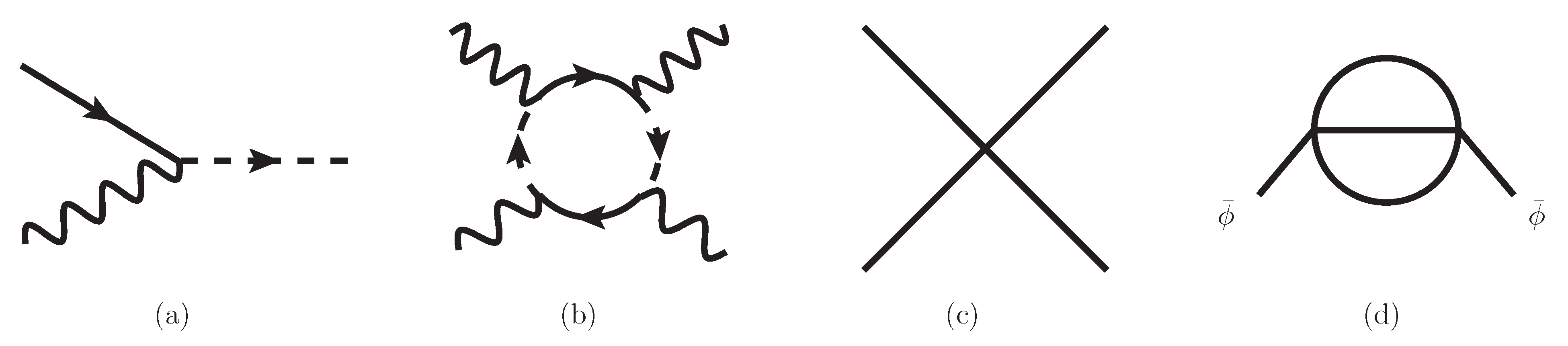
theory in a hierarchical manner for reservoir computing as a toy model for the control theory of QBD. In QBD, we adopt dipole–photon interactions as shown in
Figure 1a, where dipoles in the ground state absorb photons and dipoles then transition to the first excited states, and reverse processes are allowed to occur [
35]. Using this diagram, we can depict the loop-diagram shown in
Figure 1b, which represents photon–photon interaction with four external lines. This diagram can be represented by the interaction term in the
model in
Figure 1c. Then, the
might represent photon–photon interactions in QBD. Beginning with the Lagrangian density in the
theory, we derive the Klein–Gordon (KG) equations for the coherent field
, the expectation value of the quantum field
. The equations involve a damping term due to quantum fluctuations, which originates from the diagram in
Figure 1d in the loop-expansion [
36,
37,
38]. This damping term represents a field–particle conversion where the energy of coherent fields is transferred to that of incoherent particles. We also add an input function to the KG equations. Solving the equations with the damping term and the input function, we show how a target function is achieved by an input function. Our analysis is extended to KG equations in a hierarchy representing multiple layers covering cortex in a brain. We adopt the Klein–Gordon equations in a hierarchy involving the input, layers (reservoirs), and the output. We derive an input function to achieve the desired target function, then solve the Klein–Gordon equations with a derived input function and check whether the target function is achieved as an output function in the time-evolution dynamics of the system. The target function is found to be achieved in a hierarchy for transmission less than its threshold where signal transfer prevails above noise in intermediate layers or reservoirs. Our approach might be applied to manipulating subjective experiences in the brain by external electromagnetic fields as input functions representing external stimuli for the visual cortex, auditory cortex, somatosensory area, and so on. It might also be applied to writing or controlling our hologram memory by external electromagnetic fields. It represents non-invasive control theory for holograms or subjective experiences in Quantum Brain Dynamics, which will be the subject of a future study. If our brain would adopt the language of holography, we could also find realistic physical degrees of freedom in the contexts of quantum cognition [
39,
40,
41,
42,
43,
44] and the free-energy principle [
45,
46].
This paper is organized as follows. In
Section 2, we begin with the Lagrangian density and derive KG equations with an input function in a hierarchical manner. In
Section 3, we show how a target function is achieved in time-evolution of the KG equations by numerical simulations. In
Section 4, we discuss our numerical results and applications to manipulate holograms in QBD. In
Section 5, we provide concluding remarks and perspectives. In this paper, we use the metric tensor
in
dimensions with the Greek letters
running over 0 to
d in
dimensions and the subscripts
running over 1 to
d. The subscripts
run over 1 to
N layers in a hierarchy. We set the light speed, the Planck constant divided by
and the Boltzmann constant as 1.
2. Lagrangian Density and Klein–Gordon Equation
In this section, we begin with the Lagrangian density in the theory, show a 2-Particle-Irreducible (2PI) effective action, and derive an input–output equation, namely the Klein–Gordon (KG) equation involving input function and a damping term due to quantum fluctuations of fields obeying the Kadanoff–Baym equation. We also extend our approach to KG equations in a hierarchy.
We begin with the Lagrangian density of the
model given by
where
m represents the mass of particles and
represents the coupling constant of the interaction. We adopt the closed-time path (CTP) formalism to describe non-equilibrium phenomena in QFT. The CTP represents the path ‘1’ from
to
and the path ‘2’ from
to
[
47,
48]. Beginning with the Lagrangian density, we derive a generating functional for the connected loops of Feynman diagrams in the path integral, adopt the Legendre transformation of the generating functional, and then we can derive the 2PI effective action [
49,
50]. The 2PI effective action for this Lagrangian is derived by
with the expectation value of the background quantum field
and the Green’s function
with the notation for the expectation value
, time-ordered product
in CTP and fluctuations
. The inverse of Green’s function
in the above equation is written as
with the delta function
in CTP. Due to the Legendre transformation from the generating functional to the 2PI effective action, we can derive the following relations,
for the vanishing source terms on the right-hand side.
The Equation (
5) represents the Kadanoff–Baym equation for Green’s function
[
36,
37,
38,
51,
52] written as
with self-energy
. The Green’s function
has two independent components for anti-commutation and commutation relations of
and
, namely the statistical function
including information of particle distributions and the spectral function
involving information of dispersion relations and the spectral width, defined as
These functions can be Fourier-transformed as
in spatially homogeneous systems with times
and
. The statistical function
is symmetric
for the interchange of
t and
, while the spectral function
is anti-symmetric
.
The Equation (
4) provides the Klein–Gordon equation for coherent field
as
The term
in Equation (
11) can be absorbed to the term
. Here the Feynman diagram of
is depicted in
Figure 1d. We can show
with a spectral ‘
’ part of self-energy,
as shown in [
37,
38]. The term
in Equation (
11) can be rewritten as
where we have used the relations
and
for real
and pure imaginary
due to the anti-symmetry of
. The 2nd term in the above equation represents the damping term in the Klein–Gordon equation with the damping factor
. The damping factor appears due to the field–particle conversion where coherent fields are damped and incoherent particles described by Green’s functions are produced. It is dependent on the coupling constant
and temperature of incoherent particles with thermal equilibrium distributions or Bose–Einstein distributions. The larger the
and the temperature are, the larger the damping factor
is.
The KG equation which we should solve is given by
with the spatial label
, the input function
as an external source and the coupling constant
v. The 2nd line represents an input–output equation. When the stationary target function is given by
, the input function
is written as
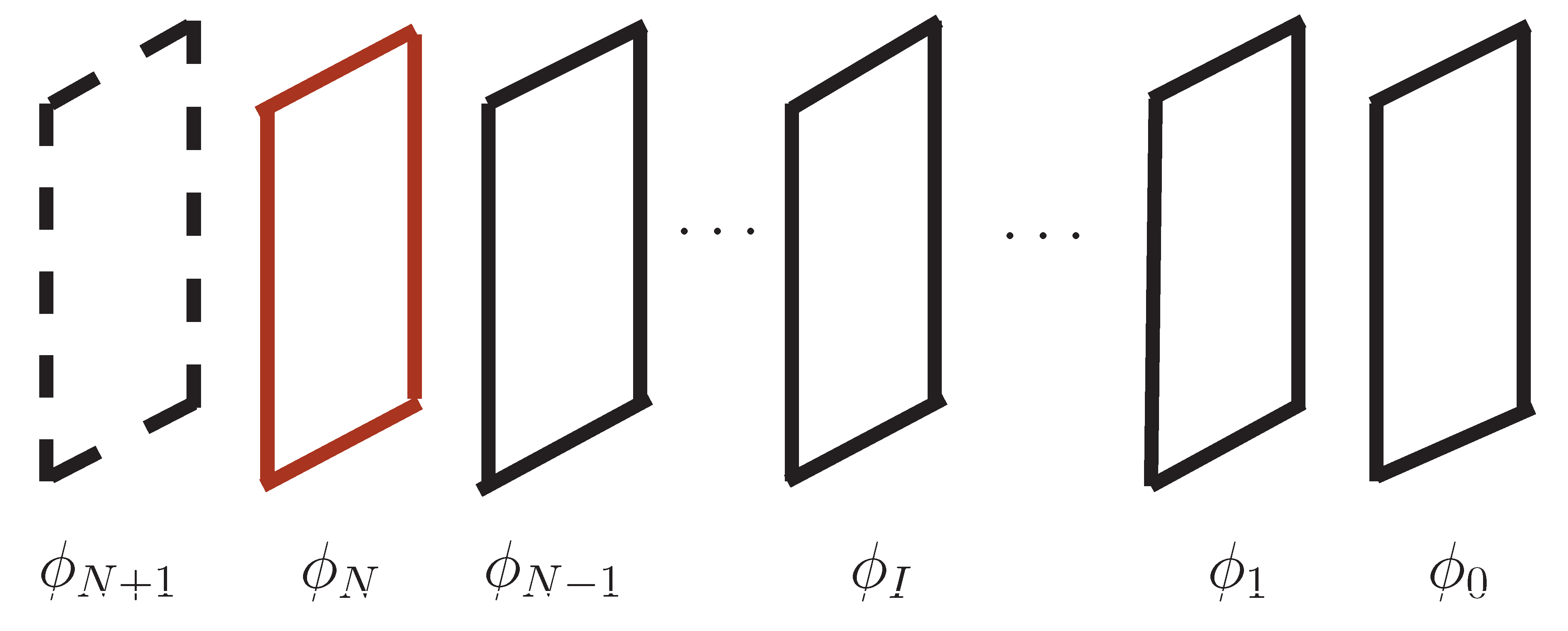
Next, we show the Klein–Gordon equation in a hierarchy in
Figure 2. The time-evolution equations in a hierarchy are,
where
with fixed
and
representing the input
. The origin of the term
is the transmission between
’s in
Ith system represented by the transmission Lagrangian term
with the transmission parameter
v. The input functions are calculated by
where
, fixed
and target function
. We use the input function
derived in Equation (
17) as a boundary condition in solving Equation (
16).
3. Numerical Results
In this section, we show how the desired target function is achieved using the Klein–Gordon equations in a hierarchy. Non-equilibrium processes are described in the time-evolution where coherent fields
, expectation values in coherent states, evolve in time. Since the time-evolving coherent fields correspond to time-evolving coherent states, dynamically evolving coherent states, involving boson condensation of an infinite number of particles on the vacua [
53], are traced in our non-equilibrium approach.
We set a two-dimensional spatial lattice by with discrete labels for with , lattice size , and lattice spacing scaled by mass m. Periodic boundary conditions for spatial coordinates are adopted. We prepare time-step as . We shall investigate the number of layers . We then prepare coupling , transmission and damping factor . To determine the time-evolution of the system, the fourth-order Runge–Kutta method is adopted.
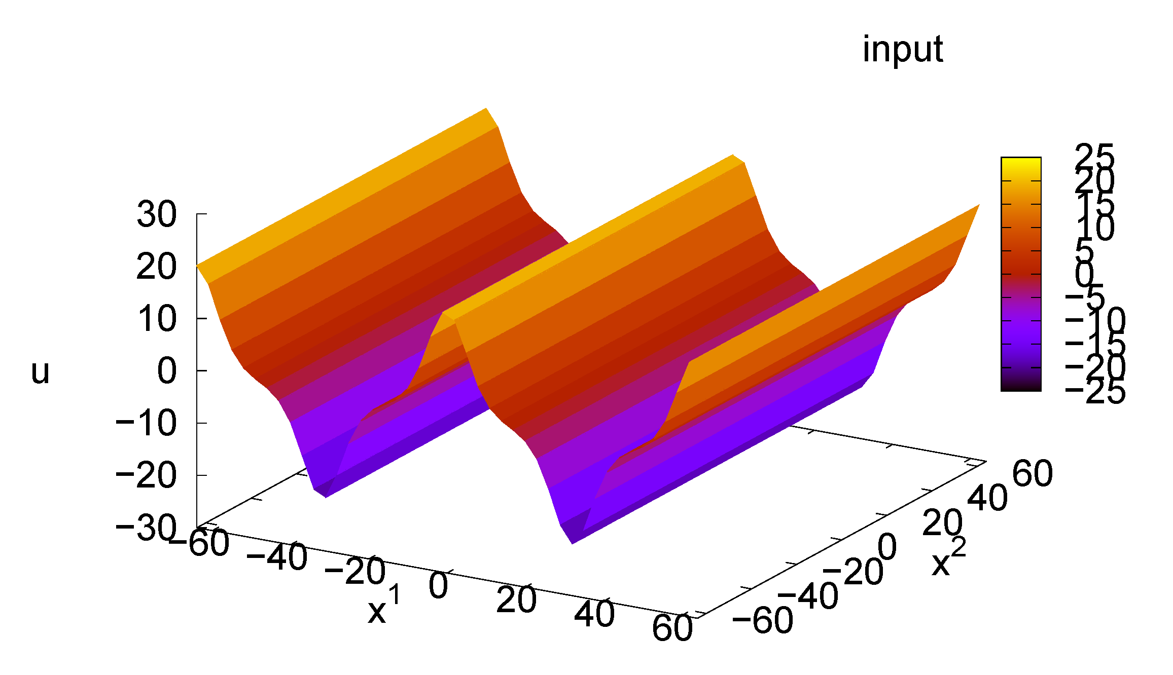
The desired target function
is set as
where we omit the scaling factor
. We calculate
using Equation (
17). The input function
for
is shown in
Figure 3. We find sawtooth waveform in
compared with the cosine curve multiplied by
in Equation (
18). The maximum value in
is approximately 20 since the input function can be approximately derived by multiplying
by the factor
, with which we find
.
We set initial conditions of
for
Ith layers
as
Initial conditions for the time derivatives are
for
. We fix
,
,
and
for any time point.
We solve Klein–Gordon equations in a hierarchy (
16) with
with
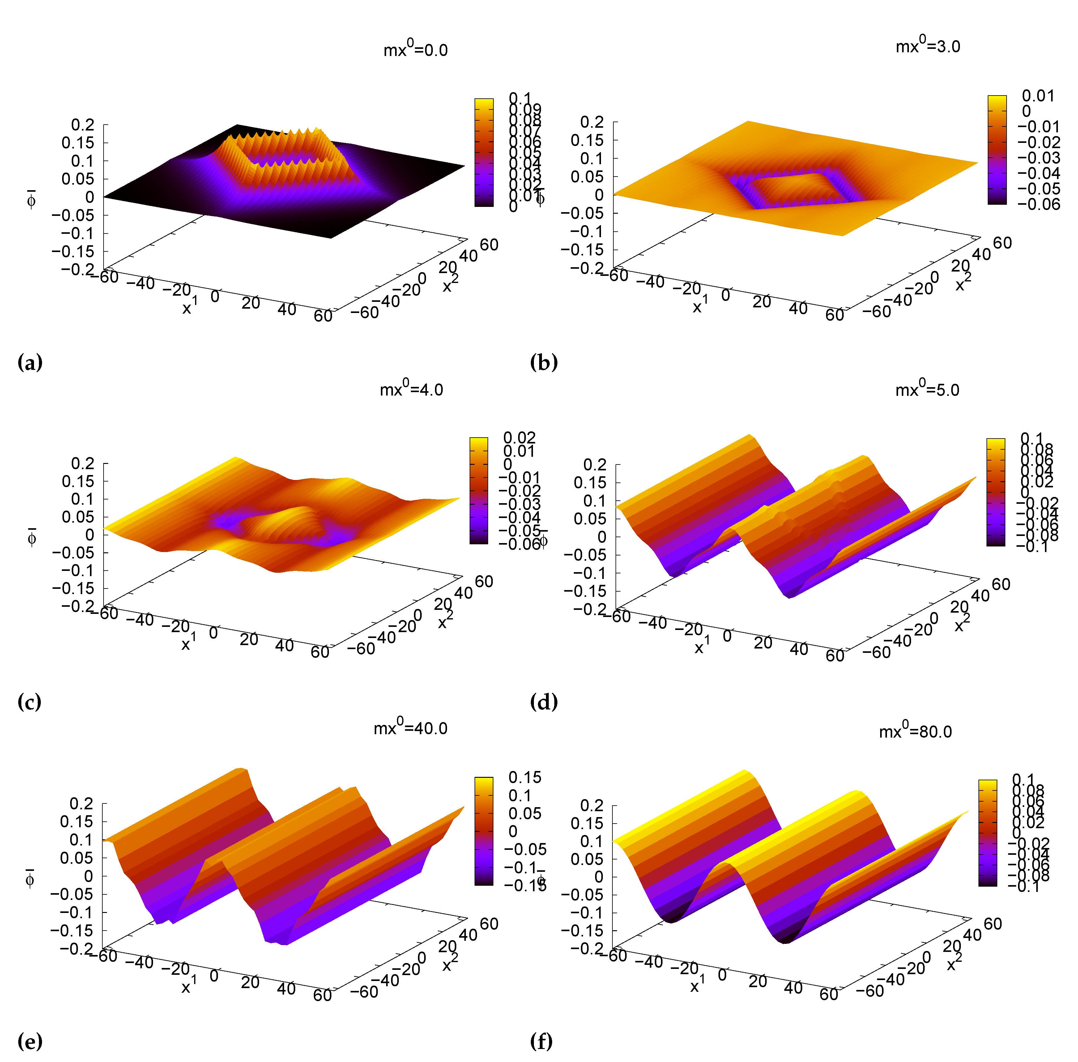
. In
Figure 4, we show the time-evolution of distributions
depicted every three spatial points. At
, we prepare a square-shaped distribution as an initial condition in Equation (
19). Its maximum value at the peaks is
. The
values at around the peaks at
start oscillating with frequency
m in their time-evolution and tend to become negative at
, which is nearly equal to
. The negative bottom is approximately
. At
, we find that the cosine curve gradually appears although the shape of the initial condition is still unchanged. At
, the shape of the initial condition tends to disappear since the inverse of the damping factor
is
. The sawtooth waveform appears at
similar to the waveform
. The shape gradually approaches the cosine curve at
. The fluctuations around the cosine curve are found to appear at this time. The values of peaks at
are larger than the amplitude
in target function
in Equation (
18). At
, the shape tends to be the target function or a cosine curve with amplitude
.
We shall investigate cases of several transmissions, namely
,
,
,
,
and
for
with
and
. In
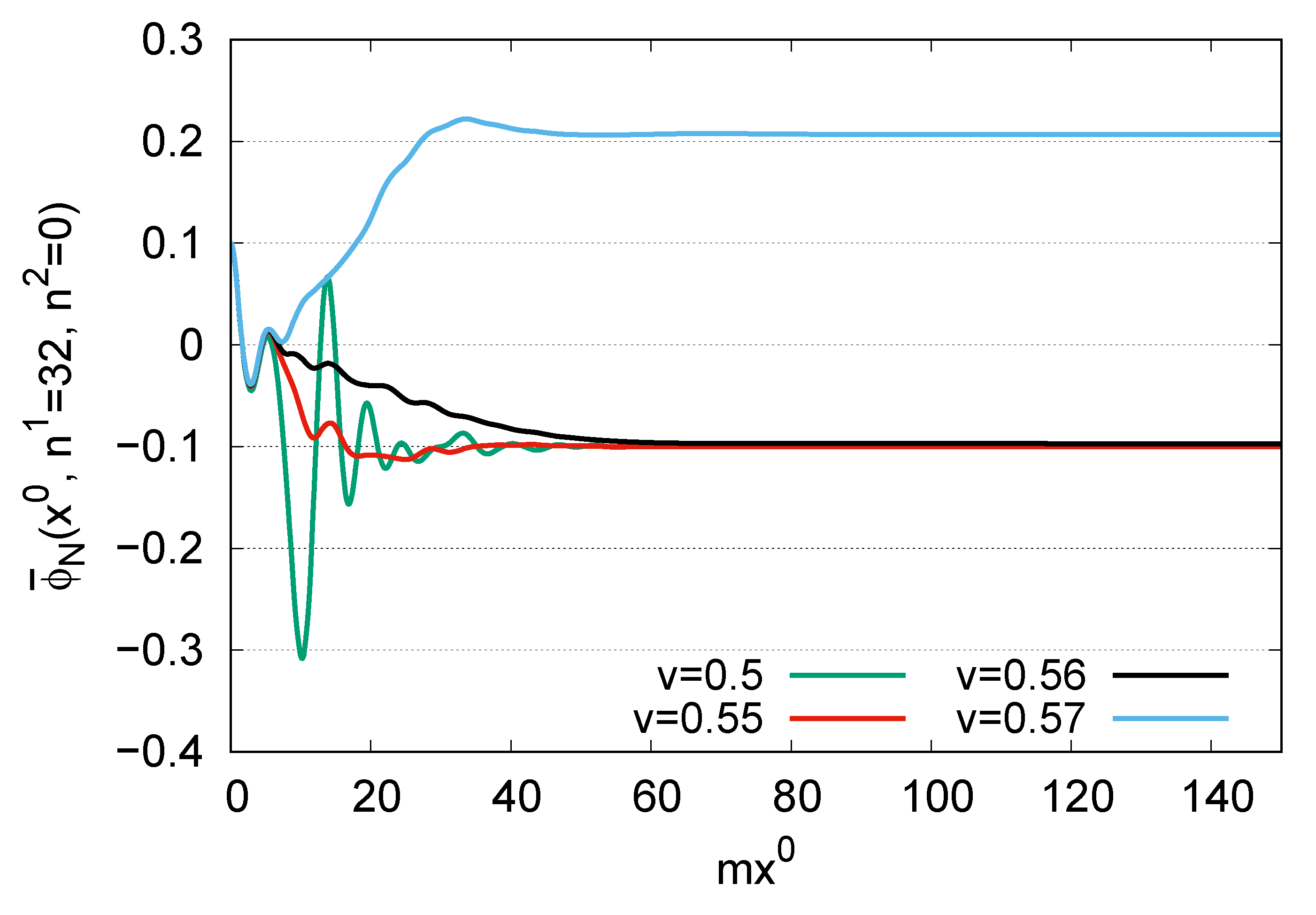
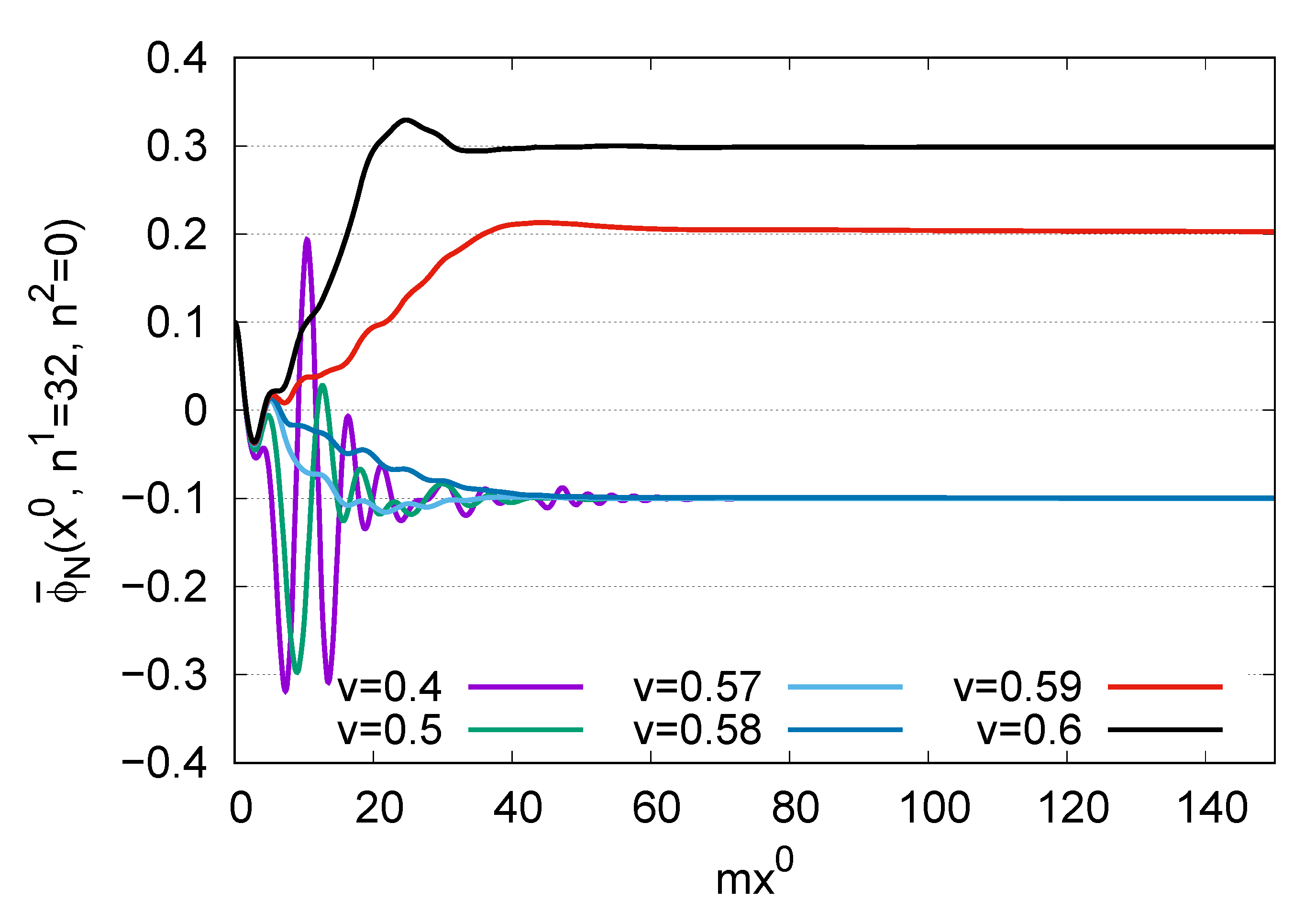
Figure 5, we show time-evolution of
. We can check the convergence properties of coherent fields. Due to
in Equation (
19) and
in Equation (
18),
starts from
and converges to
in the course of time-evolution if the target function is achieved. For
and
, the
converges to
. The fluctuations of the target functions seem to be larger for smaller transmission
v. On the contrary, it converges to approximately
and
for
and
, respectively. Then the
does not converge to the target function
in Equation (
18).
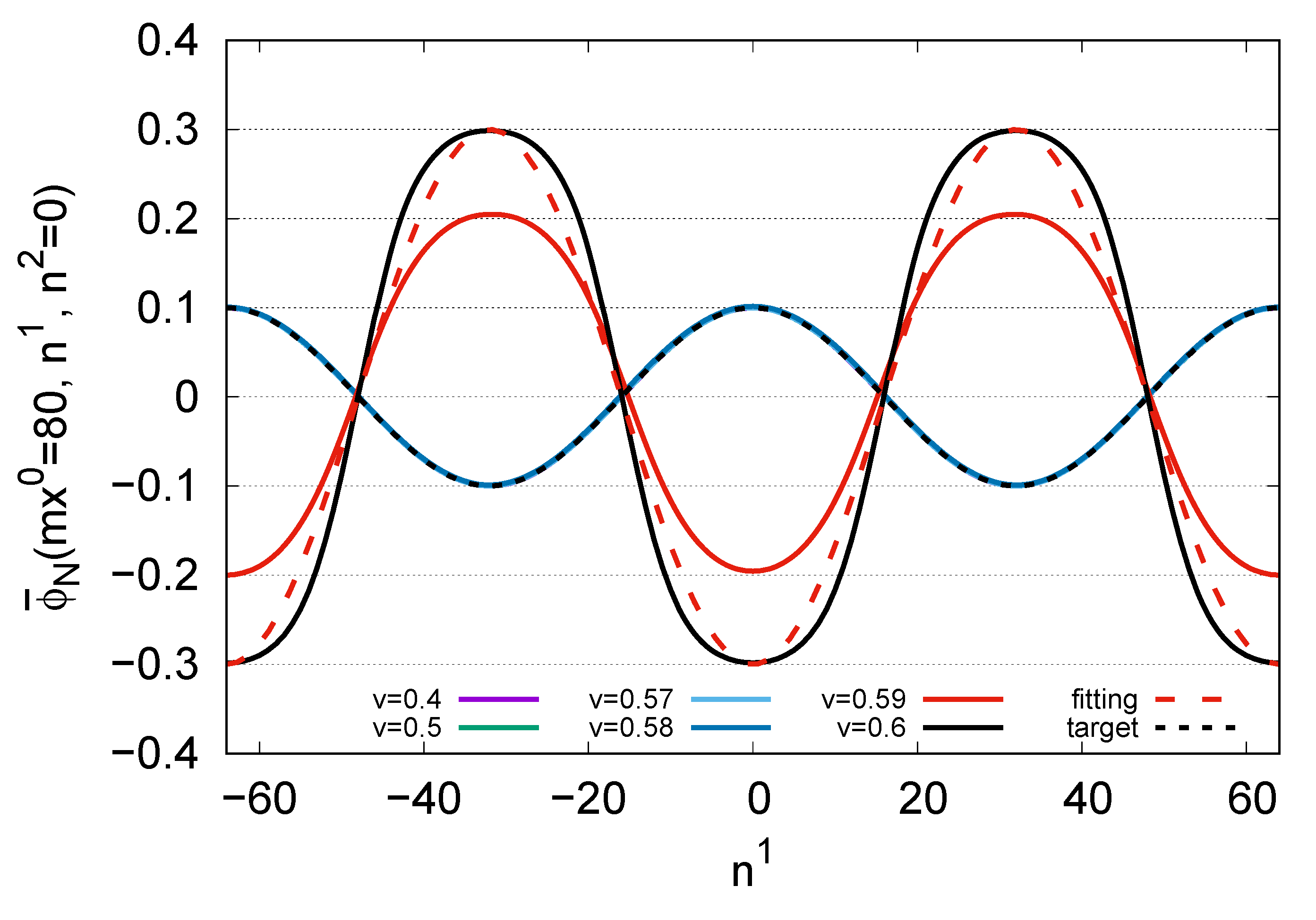
In
Figure 6, we show the distribution of the coherent field for
,
,
,
,
and
for
, We find that
’s at
for
and
converge to the target function. The deviations from the target function cannot be clearly seen. Contrary to that,
’s at
for
and
do not have the waveform of the target function. Comparing it with the cosine function
for
, we find that the shape seems to be near step-function-like forms. The threshold of whether the convergence to the target function is achieved is approximately
.
We shall also investigate cases for
for the target function in Equation (
18) and initial conditions in Equations (
19) and (
20). We investigate several cases of transmissions
,
,
, and
with
and
. In
Figure 7, we show the time-evolution of
for
,
,
, and
for
. For
,
, and
, the
starts from
and tends to converge to
. As we decrease
, fluctuations in the time-evolution become larger. On the contrary,
tends to converge to
for
. This means that
does not converge to the target function for
. The threshold of whether the convergence to the target function is achieved in the time-evolution is approximately
. As the number of layers
N increases, the threshold for
v seems to decrease gradually.
4. Discussion
In this paper, we have investigated non-equilibrium theory in a hierarchy as a toy model of control theory to manipulate holograms in Quantum Brain Dynamics (QBD). We have introduced the Lagrangian density of theory and derived the Klein–Gordon (KG) equation with a damping term, which originated from the field–particle conversion where damped oscillations of coherent fields occur and incoherent particles are produced from coherent fields. We have added an input function u as an external source of coherent fields, which might represent an external electromagnetic field in QBD. We have subsequently extended the equation to the KG equations in a hierarchy representing layers covering the cortex area in the human brain, where the number of layers is N. Then, we have derived the input function to achieve the convergence to the desired target function in Nth layer. Using the derived input function and solving KG equations, we have investigated whether the coherent field in the Nth layer converges to the target function in time-evolution using numerical simulations. We have found that the convergence to the target function can be achieved for the transmission parameter v whose value is below the threshold.
We discuss the convergence and uniqueness in time-evolution of coherent fields. It is straightforward to investigate the case
. Substituting the input function in Equation (
15) into the input–output Equation (
14), we can derive the following time-evolution equation,
with
. The above equation, except for the nonlinear term
, represents the damped oscillation for
in time-evolution. Since
converges to zero in time-evolution, the
converges to the target function
. Even if a nonlinear term exists, the results for convergence do not change. Since
is a monotonically increasing function for
,
has one-to-one correspondence to
. When
is equal to
,
is equal to
. (Or, since we can write
, a nonlinear term will be a correction term to
in damped oscillations.) Then, the uniqueness of the output function in convergence is achieved for a given target function
.
For the number of layers
in a hierarchy, we found the threshold for the transmission parameter
v of whether the convergence to target function is achieved. When transmission
v is less than the threshold, the convergence to the target function is achieved. The threshold in a hierarchy might be estimated as follows. We first investigate the time-evolution equation,
The solution of this equation can be written as
with
with constants
A and
B, and with the Fourier transformation
. When
is time-independent, we find
due to
. The output
is expressed as the sum of
and the external input
u. We next investigate the time-evolution equation,
in a hierarchy. In a similar way to the above derivation, we find,
where
represents
with constants
and
and we have omitted the scaling factor
. In
, the output function
can be expanded as
Here, due to
, we can show
. In the above equation, the first and second terms on the right-hand side represent the signal information. On the other hand, the third, fourth, fifth and sixth terms in intermediate layers are regarded as noise. We shall estimate the order of signal and noise by taking a sum of coefficients where the coefficient in
is 1. The signal and noise function with
and
are written as
as a function of transmission parameter
v. We show the values of the signal and noise function in
Table 1.
In this table, we find that
prevails over
in
. Yet,
prevails over
in
and
. The threshold for whether the convergence to the target function is achieved is
in numerical simulations for
in the previous section. The threshold for numerical simulations corresponds to the upper limit where
prevails over
in
Table 1. We also investigate the case
. In a similar way to the above derivation, we can derive,
We then find
for
. We show
and
in
Table 2.
In this table, we find that prevails over in . This value corresponds to the upper limit for the convergence to the target function in the previous section. We might be able to derive the threshold in the above analysis. As the number of layers increases, the threshold decreases gradually. To achieve the convergence to the target function, small transmission parameters where signal prevails over noise are required. In controlling holograms or subjective experiences in the brain, we might qualitatively need to select electromagnetic waves with smaller transmission and external electromagnetic fields above the threshold. If transmission of magnetic fields is large in the brain where the noise prevails over signal, we propose to select electric fields with small transmission.
The geometry is also of significance for control theory. In this paper, we investigate flat two-dimensional surfaces or multiple flat layers in a hierarchy. Manipulating holograms in a flat surface, we propose to control our subjective experiences and to overwrite memory by external electromagnetic fields non-invasively. However, if holographic memory is not on flat surfaces, the situations for control theory will change. There are several structures that might memorize information, such as spherical, toroidal and cylindrical shapes for neurons, glia cells and microtubules as a candidate structures to record memory. To control holograms with these structures, we might need a hemispherical surface headset covering our head to achieve the convergence to the target functions on three-dimensional structures for cells and their cytoskeletons. We then need three-dimensional control theory to construct target functions for target areas in the brain.
McFadden proposed a conscious electromagnetic information field in [
54,
55]. Electromagnetic fields might be a candidate to solve the binding problem, namely how the brain integrates parallel processing in various diffused areas. Since electromagnetic fields without media propagate at the speed of light and are not localized, we need to introduce media with water dipoles so that photons acquire a mass in the brain [
1]. We can adopt the Higgs mechanism in QBD where Nambu–Goldstone modes are absorbed by photons fields and photons acquire mass. The massive photons are called evanescent photons. The maximum mass is found to be
with the dipole moment of a water molecule
(elementary charge
and the distance
Å), the moment of inertia
I with
and the number density of coherent water
by estimating the Meissner effect of electric fields in the Klein–Gordon equations [
35]. Then, we might be able to adopt the integrated version of the holographic brain theory proposed by Pribram and QBD with water dipoles and evanescent photons. Our subjective experiences and memories might be represented by holograms within this type of theory. To investigate whether our brain encodes information using the language of holography, we need the control theory of holograms using external electromagnetic fields.
When our memory-inducing subjective experiences are manipulated, we might find one-to-one correspondence between subjective experiences in the mind and holograms constructed in physical light–matter systems in the brain. Our approach might represent a reductionism of subjective experiences to holograms induced by quantum fields with light–matter, or contribute to mind–matter unification in panpsychism. Mind–light–matter unification is proposed in [
56], where light plays a role of the bridge between mind and matter. Mind–matter unification would be impossible without the bridging role of light. As suggested in [
57], “quantum intelligence” (QI), a novel quantum-computing prototype, aims to clarify the concept of causality. We could then reach logically definable causality and mind–light–matter unity. Holographic extension using bipolar qubits in QI is also possible. One could adopt a holographic approach to brain dynamics involving logical reasoning provided by logically definable causality. The mind–brain relationship might be described in quantum theory where measurement processes convert several possibilities in superposition states to actual observed events acausally, as proposed in [
58]. Quantum approaches break the causal closure of deterministic Newtonian or Classical mechanics and provide new explanations of mind and matter.
When our brain adopts the language of holography, we can provide realistic physical degrees of freedom for quantum cognition and the free-energy principle. In quantum cognition, quantum-like mathematical models are adopted for our decision-making not as physico-chemical approach but as information-theoretical approach [
39,
40,
41,
42,
43,
44]. Quantum interference between states describes irrational decision-making with fallacy, the violation of the sure-thing principle, quantum-like information processing, and so on. The free-energy principle as a mathematical approach suggests that our brain function adopts the minimization of free energy in biological information processing [
45,
46]. The minimization of free energy is related to Bayesian inference in which causes of events
c with the prior probability
are inferred by given data
d in resultant events in Bayes’ theorem. This minimization indicates the case that the posterior probability
(conditional probability of causes
c in given data
d occurring) = the prior probability
. In adopting the excess Bayesian inference involving a quantum logic implemented in [
59] instead of classical Bayesian inference, the free-energy principle is connected to quantum cognition. Although quantum-like states are adopted in a mathematical model on quantum cognition, we can assign holograms (constructed by realistic physical degrees of freedom of light–matter) to quantum-like states in quantum cognition. We consider the superposition state of a photon propagating in two pathways
and
. If the 0 and 1 pathways are exposed on holograms 0 and 1, respectively, we can consider the entanglement given by
for photons in propagating through holograms 0 and 1. In holography, the optical information propagating through holograms can perform information processing by filtering. After filtering processes, the quantum state of a photon might be processed as
Due to the measurement processes, the decision is made. Increasing the number of photons, we then take the ensemble average and find the probability of our decisions. Although we have investigated the control theory in model as a toy model of a light–matter system in this paper, our approach will be extended to more realistic QBD. We could then provide realistic physical degrees of freedom in the contexts of quantum cognition and the free-energy principle.


