Operatorial Formulation of a Model of Spatially Distributed Competing Populations

Abstract

This paper deals with the application of the mathematical apparatus of quantum mechanics for the formulation of an operatorial model of a couple of populations spatially distributed over a one-dimensional region. The two populations interact with a competitive mechanism and are able to diffuse over the region. A nonlocal competition effect is also included. In more detail, we consider a one-dimensional region divided in N cells where the actors, represented by annihilation, creation, and a number fermionic operators, interact. The dynamics is governed by a self-adjoint and time-independent Hamiltonian operator describing the various interactions. The results of some numerical simulations are presented and discussed. The recently introduced variant of the standard Heisenberg approach, named $(\mathcal{H},\rho )$-induced dynamics, is also used in order to take into account some changes in time of the attitudes of the two populations, and obtain more realistic dynamical outcomes.

1. Introduction

The dynamics of different interacting species or populations occupying the same habitat is an important subject in theoretical biology. When two like populations share the same ecological niche, Gause’s law of competitive exclusion says that the less fitted population goes extinct. Nevertheless, this law can be violated in a patchy environment, where the coexistence may occur because of migration. In fact, the less fitted population may survive even in presence of a more competitive population provided that it is able to move more effectively towards unoccupied patches so balancing local extinction in some patches [1,2,3,4,5].

In the literature, the dynamics of spatially distributed interacting populations is often modeled in terms of reaction–diffusion partial differential equations [6], or using the coupled map lattice formalism. In both approaches, various behaviors can be observed, such as pattern formation in the distributions of the competing species, and/or synchronization effects between the phases of nearby regions.

In this paper, we use a different approach relying on the mathematical apparatus originally developed in quantum mechanics [7,8]. This because, in recent years, raising and lowering operators, and the so-called number representation, were successful in the mathematical modeling of several kinds of macroscopic systems outside physics (see [9,10,11,12,13,14,15,16,17,18,19,20,21,22,23,24], and references therein, where the main motivations suggesting the use of the tools originally developed in a quantum context to describe classical situations have been widely discussed). Therefore, in such a framework, the actors of the system we want to study are described by operators in a Hilbert space and not by ordinary functions. It is worth of being remarked that operatorial models for competing populations spatially distributed and able to migrate have been already proposed [25,26,27].

In this paper, we consider a system where two different populations in a patchy environment compete either locally (in the same cell) or nonlocally (in adjacent cells) and both are subject to migration phenomena with different mobilities. With respect to previous operatorial models for describing the dynamics of interacting populations, our description includes also a nonlocal competition mechanism. Moreover, in addition to the standard Heisenberg view to dynamics, we use also the approach of $(\mathcal{H},\rho )$-induced dynamics (see [28,29,30,31], and references therein).

To the actors of the model we associate fermionic operators. This choice has two main motivations. The first one is of technical nature: in fact, the Hilbert space where the fermionic operators live is finite-dimensional, so that all the observables are bounded operators. The second one is concerned with the interpretation: the mean values of the observables (the number operators) over an initial condition can be thought of as local densities of the populations in the different cells [25].

The plan of the paper is the following. In Section 2, for the reader’s convenience, we briefly review few useful notions about quantum mechanics and the number representation for fermions. Then, we present our model, whose dynamics is assumed to be governed by a time-independent self-adjoint quadratic Hamiltonian operator: competition (both local and nonlocal) as well as migration effects are taken into account. The quadratic expression of the Hamiltonian implies that the differential equations, derived according to Heisenberg view, are linear, so that, at least formally, we can deduce analytically the solution. Section 2.1 briefly describes the $(\mathcal{H},\rho )$-induced dynamics framework, and how this approach is used in our model. We also discuss the (social) meaning of the rules we use. In Section 3, we present some numerical simulations obtained by considering two different scenarios, and discuss the results, both in the case of the standard Heisenberg dynamics and when the method of $(\mathcal{H},\rho )$-induced dynamics is used; the latter approach studies the evolution of the system, as ruled by the Hamiltonian, but with the action, at fixed instants, of some rules whose effect is that of modifying the values of some parameters entering the Hamiltonian (without modifying the structure of the Hamiltonian) as a consequence of the evolution of the system itself. In such a way, the model adjusts itself during the evolution; the introduction of such a variant can be thought of as a surreptitious way of describing the change of the attitudes of the populations during the evolution, without introducing a time dependence in the Hamiltonian or opening the system to the environment by considering a reservoir [32,33], so without additional technical difficulties. Various sets of rules are considered. In some applications already studied [28,29], the effect of the rules was that of allowing the system to approach asymptotic equilibrium states. Nevertheless, we observe that this behavior is not necessarily exhibited in our spatially distributed model, even if it introduces a sort of irreversibility in the evolution. Different sets of parameters and initial conditions are used, and the numerical results are discussed. Finally, Section 4 contains our concluding remarks, as well as some future extensions of the model to a two-dimensional spatial setting.

2. The Operatorial Model: Heisenberg Dynamics and $(\mathcal{H},\mathbf{\rho })$-Induced Dynamics

In this Section, after briefly reviewing the basic notions of the fermionic operatorial formalism, we introduce the model we are interested in. We describe the actors of our system as well as their interactions embedded in a Hamiltonian operator. Then, adopting the Heisenberg viewpoint, we derive the differential equations ruling the dynamics.

The system $\mathcal{S}$ we consider consists of two populations occupying a one-dimensional spatial region $\mathcal{C}$ composed by N cells; in each cell, two different populations, say ${\mathcal{P}}_1$ and ${\mathcal{P}}_2$, coexist and interact. Let $a_{1,\alpha }$ and $a_{2,\alpha }$ ($a_{1,\alpha }^{†}$ and $a_{2,\alpha }^{†}$, respectively) be the annihilation (creation, respectively) fermionic operators related to the two populations, where the subscript $\alpha$ is a label for the cells of the spatial region; moreover, let ${\widehat{n}}_{j,\alpha }=a_{j,\alpha }^{†}{a}_{j,\alpha }$ be the corresponding number operators. According to the formalism of second quantization, annihilation and creation operators satisfy the canonical anticommutation relations

$$\{a_{j,\alpha },a_{k,\beta }\}=\{a_{j,\alpha }^{†},a_{k,\beta }^{†}\}=0,\{a_{j,\alpha },a_{k,\beta }^{†}\}={\delta }_{j,k}{\delta }_{\alpha ,\beta }\mathcal{I},$$

(1)

$j,k=1,2$, $\alpha ,\beta =1,\dots ,N$, $\mathcal{I}$ being the identity operator, ${\delta }_{j,k}$ and ${\delta }_{\alpha ,\beta }$ the Kronecker symbols, and $\{u,v\}:=uv+vu$ the anticommutator between the operators u and v. The Hilbert space $\mathbb{H}$, where the operators are defined, is constructed as the linear span of the orthonormal set of vectors

$${\phi }_{{\mathbf{n}}_1,{\mathbf{n}}_2}={\left(a_{1,1}^{†}\right)}^{n_{1,1}}\cdots {\left(a_{1,N}^{†}\right)}^{n_{1,N}}{\left(a_{2,1}^{†}\right)}^{n_{2,1}}\cdots {\left(a_{2,1}^{†}\right)}^{n_{2,N}}{\phi }_{\mathbf{0},\mathbf{0}},$$

(2)

i.e., ${\phi }_{{\mathbf{n}}_1,{\mathbf{n}}_2}\equiv {\phi }_{n_{1,1},\dots ,n_{1,N},n_{2,1}\dots ,n_{2,N}}$ is obtained by acting on the vacuum ${\phi }_{\mathbf{0},\mathbf{0}}\equiv {\phi }_{0,0,\dots ,0}$ (i.e., the vector annihilated by all $a_{j.\alpha }$) with the powers of the operators $a_{j,\alpha }^{†}$, where $n_{j,\alpha }=0,1$. As a consequence, $\dim \left(\mathbb{H}\right)=2^{2N}$.

The vector ${\phi }_{{\mathbf{n}}_1,{\mathbf{n}}_2}$ means that to the j-th population in the cell $\alpha$, a mean value equal to $n_{j,\alpha }$ is initially assigned such that

$${\widehat{n}}_{j,\alpha }{\phi }_{{\mathbf{n}}_1,{\mathbf{n}}_2}=n_{j,\alpha }{\phi }_{{\mathbf{n}}_1,{\mathbf{n}}_2}.$$

(3)

The mean values of number operators over an initial condition ${\phi }_{{\mathbf{n}}_1,{\mathbf{n}}_2}$, say

$$n_{j,\alpha }=\langle {\phi }_{{\mathbf{n}}_1,{\mathbf{n}}_2},{\widehat{n}}_{j,\alpha }{\phi }_{{\mathbf{n}}_1,{\mathbf{n}}_2}\rangle ,j=1,2,\alpha =1,\dots ,N$$

(4)

are interpreted as the local density of the population ${\mathcal{P}}_j$ in the cell $\alpha$.

Let us assume the dynamics to be governed by a self-adjoint time-independent Hamiltonian operator $\mathcal{H}$. Its definition embodies the interactions among the agents of the system:

$$\mathcal{H}={\mathcal{H}}_0+{\mathcal{H}}_I+{\mathcal{H}}_C+{\mathcal{H}}_M,$$

(5)

where

$$\left\{\begin{array}{cc}\hfill & {\mathcal{H}}_0=\sum _{j=1}^2\sum _{\alpha =1}^N{\omega }_{j,\alpha }{a}_{j,\alpha }^{†}{a}_{j,\alpha },\hfill \\ \hfill & {\mathcal{H}}_I=\sum _{\alpha =1}^N{\lambda }_{\alpha }(a_{1,\alpha }{a}_{2,\alpha }^{†}+a_{2,\alpha }{a}_{1,\alpha }^{†}),\hfill \\ \hfill & {\mathcal{H}}_C=\sum _{\alpha =1}^N\left({\nu }_{\alpha }\sum _{\beta =1}^N{p}_{\alpha ,\beta }(a_{1,\alpha }{a}_{2,\beta }^{†}+a_{2,\beta }{a}_{1,\alpha }^{†})\right),\hfill \\ \hfill & {\mathcal{H}}_M=\sum _{j=1}^2\sum _{\alpha =1}^N\left({\mu }_{j,\alpha }\sum _{\beta =1}^N{p}_{\alpha ,\beta }(a_{j,\alpha }{a}_{j,\beta }^{†}+a_{j,\beta }{a}_{j,\alpha }^{†})\right),\hfill \end{array}\right.$$

(6)

with ${\omega }_{j,\alpha }$, ${\lambda }_{\alpha }$, ${\mu }_{j,\alpha }$, ${\nu }_{\alpha }$ ($\alpha =1,\dots ,N$, $j=1,2$) positive constants; moreover, the coefficients $p_{\alpha ,\beta }$ ($\alpha ,\beta =1,\dots ,N$), symmetric with respect to their indices, are equal to 1 if $\beta$ denotes a cell in the Moore neighborhood $M_{\alpha }$ (the set of adjacent cells) and 0 elsewhere. Thus, the cells in the Moore neighborhood of the cell $\alpha \ne 1,N$ are labeled as $\alpha -1$ and $\alpha +1$, whereas the cells labeled with 1 and N have only one neighbor (labeled 2 and $N-1$, respectively).

Some comments about the various contributions in the Hamiltonian are in order:

• ${\mathcal{H}}_0$ is the free part of the Hamiltonian, and ${\omega }_{j,\alpha }$ are parameters that can be interpreted as a measure of the inertia of the operators associated to the agents of $\mathcal{S}$: in fact, they can be thought of as a measure of the tendency of each degree of freedom to stay constant in time [9].
• ${\mathcal{H}}_I$ accounts for the local (i.e., in the same cell $\alpha$) competitive interaction between the two populations; the coefficients ${\lambda }_{\alpha }$ give a measure of the strength of the interaction, and, when ${\lambda }_{\alpha }=0$ for all $\alpha$, there is no competition at all: the contribution $a_{1,\alpha }{a}_{2,\alpha }^{†}$ is a competition term since the actor associated to $a_{1,\alpha }$ is destroyed and the actor associated to $a_{2,\alpha }$ is created; the adjoint term $a_{2,\alpha }{a}_{1,\alpha }^{†}$ swaps the roles of the two actors.
• ${\mathcal{H}}_C$ takes into account a nonlocal competitive interaction between the two populations, and ${\nu }_{\alpha }$ measures the strength of nonlocal interaction (absent if ${\nu }_{\alpha }=0$, $\alpha =1,\dots ,N$): in fact, the competition between the two populations occurs in adjacent cells.
• ${\mathcal{H}}_M$ is responsible for the diffusion of the two populations in the region, and ${\mu }_{j,\alpha }$ is the mobility coefficient of population ${\mathcal{P}}_j$ in the cell $\alpha$: the contribution $a_{j,\alpha }{a}_{j,\beta }^{†}$ is such that the actor associated to $a_{j,\alpha }$ is destroyed and the actor associated to $a_{j,\beta }$ is created; once again, the adjoint term $a_{j,\beta }{a}_{j,\alpha }^{†}$ swaps the roles of the two actors.

The choice (that could seem too much restrictive) of considering a one-dimensional spatial region where the two populations interact and—with different mobilities—migrate is not just (or only) a trick to simplify the analysis. In fact, migratory phenomena are often observed along well-defined directions, e.g., from south to north; in such circumstances, a model where the two populations are assumed spatially distributed in a one–dimensional region can result appropriate.

Adopting the Heisenberg representation, the operators $a_{j,\alpha }$ evolve in time according to the differential equations

$$\frac{d{a}_{j,\alpha }}{dt}=\mathrm{i}[\mathcal{H},a_{j,\alpha }],$$

(7)

where $[\mathcal{H},a_{j,\alpha }]=\mathcal{H}{a}_{j,\alpha }-a_{j,\alpha }\mathcal{H}$ is the commutator between $\mathcal{H}$ and $a_{j,\alpha }$. Using (7), because of the quadratic form of the Hamiltonian operator, we get a linear system of ordinary differential equations, say

$$\begin{array}{cc}\hfill & \frac{d{a}_{1,\alpha }}{dt}=\mathrm{i}\left(-{\omega }_{1,\alpha }{a}_{1,\alpha }+{\lambda }_{\alpha }{a}_{2,\alpha }+\sum _{\beta \in M_{\alpha }}\left(({\mu }_{1,\alpha }+{\mu }_{1,\beta })a_{1,\beta }+{\nu }_{\alpha }{a}_{2,\beta }\right)\right),\hfill \\ \hfill & \frac{d{a}_{2,\alpha }}{dt}=\mathrm{i}\left(-{\omega }_{2,\alpha }{a}_{2,\alpha }+{\lambda }_{\alpha }{a}_{1,\alpha }+\sum _{\beta \in M_{\alpha }}\left(({\mu }_{2,\alpha }+{\mu }_{2,\beta })a_{2,\beta }+{\nu }_{\beta }{a}_{1,\beta }\right)\right),\hfill \end{array}$$

(8)

for $\alpha =1,\dots ,N$. In our one-dimensional setting, system (8) becomes:

$$\begin{array}{cc}\hfill \frac{d{a}_{1,1}}{dt}& =\mathrm{i}\left(-{\omega }_{1,1}{a}_{1,1}+{\lambda }_1{a}_{2,1}+({\mu }_{1,1}+{\mu }_{1,2})a_{1,2}+{\nu }_1{a}_{2,2}\right),\hfill \\ \hfill \frac{d{a}_{1,\alpha }}{dt}& =\mathrm{i}\left(-{\omega }_{1,\alpha }{a}_{1,\alpha }+{\lambda }_{\alpha }{a}_{2,\alpha }+({\mu }_{1,\alpha }+{\mu }_{1,\alpha -1})a_{1,\alpha -1}+({\mu }_{1,\alpha }+{\mu }_{1,\alpha +1})a_{1,\alpha +1}\right.\hfill \\ \hfill & \left.+{\nu }_{\alpha }(a_{2,\alpha -1}+a_{2,\alpha +1})\right),\alpha =2,\dots ,N-1,\hfill \\ \hfill \frac{d{a}_{1,N}}{dt}& =\mathrm{i}\left(-{\omega }_{1,N}{a}_{1,N}+{\lambda }_N{a}_{2,N}+({\mu }_{1,N}+{\mu }_{1,N-1})a_{1,N-1}+{\nu }_N{a}_{2,N-1}\right),\hfill \\ \hfill \frac{d{a}_{2,1}}{dt}& =\mathrm{i}\left(-{\omega }_{2,1}{a}_{2,1}+{\lambda }_1{a}_{1,1}+({\mu }_{2,1}+{\mu }_{2,2})a_{2,2}+{\nu }_2{a}_{1,2}\right),\hfill \\ \hfill \frac{d{a}_{2,\alpha }}{dt}& =\mathrm{i}\left(-{\omega }_{2,\alpha }{a}_{2,\alpha }+{\lambda }_{\alpha }{a}_{1,\alpha }+({\mu }_{2,\alpha }+{\mu }_{2,\alpha -1})a_{2,\alpha -1}+({\mu }_{2,\alpha }+{\mu }_{2,\alpha +1})a_{2,\alpha +1}\right.\hfill \\ \hfill & \left.+{\nu }_{\alpha -1}{a}_{1,\alpha -1}+{\nu }_{\alpha +1}{a}_{1,\alpha +1}\right),\alpha =2,\dots ,N-1,\hfill \\ \hfill \frac{d{a}_{2,N}}{dt}& =\mathrm{i}\left(-{\omega }_{2,N}{a}_{2,N}+{\lambda }_N{a}_{1,N}+({\mu }_{2,N}+{\mu }_{2,N-1})a_{2,N-1}+{\nu }_{N-1}{a}_{1,N-1}\right).\hfill \end{array}$$

(9)

The unknowns in (9) are operators represented by $2^{2N}\times 2^{2N}$ matrices with complex entries, whereupon, at least in principle, we have to solve a system of $2N\times 2^{4N}$ scalar ordinary differential equations in the complex domain. Nevertheless, because of the linearity of Equation (9), we are able to reduce drastically the computational complexity. In fact, introducing the formal column vector

$$\mathbf{A}={\left[a_{1,1},\dots ,a_{1,N},a_{2,1},\dots ,a_{2,N}\right]}^T,$$

(10)

(${}^T$ stands for the transposition operator) and a suitable $2N\times 2N$ real matrix $\mathsf{\Gamma }$ (whose entries, once we fix N, can be constructed from (9)), the evolution equations for the annihilation operators can be written in the compact form as

$$\frac{d\mathbf{A}}{dt}=\mathrm{i}\mathsf{\Gamma }\mathbf{A}.$$

(11)

Let us now consider the compact version of the evolution equations for the creation operators, say

$$\frac{d{\mathbf{A}}^{†}}{dt}=-\mathrm{i}\mathsf{\Gamma }{\mathbf{A}}^{†};$$

(12)

coupling (11) and (12), we have the system

$$\frac{d}{dt}\left[\begin{array}{c}\mathbf{A}\hfill \\ {\mathbf{A}}^{†}\hfill \end{array}\right]=\left[\begin{array}{cc}\mathrm{i}\mathsf{\Gamma }\hfill & {\mathbf{0}}_{2N}\hfill \\ {\mathbf{0}}_{2N}\hfill & -\mathrm{i}\mathsf{\Gamma }\hfill \end{array}\right]\left[\begin{array}{c}\mathbf{A}\hfill \\ {\mathbf{A}}^{†}\hfill \end{array}\right],$$

(13)

where ${\mathbf{0}}_{2N}$ is a zero matrix of order $2N$; actually, we do not need to consider the equations for the creation operators, but this simplifies the formulae for the mean values of the number operators (see below).

The formal solution to system (13) is

$$\left[\begin{array}{c}\mathbf{A}\left(t\right)\hfill \\ {\mathbf{A}}^{†}\left(t\right)\hfill \end{array}\right]=exp\left(\left[\begin{array}{cc}\mathrm{i}\mathsf{\Gamma }t\hfill & {\mathbf{0}}_{2N}\hfill \\ {\mathbf{0}}_{2N}\hfill & -\mathrm{i}\mathsf{\Gamma }t\hfill \end{array}\right]\right)\left[\begin{array}{c}{\mathbf{A}}_0\hfill \\ {\mathbf{A}}_0^{†}\hfill \end{array}\right]=\mathcal{B}\left(t\right)\left[\begin{array}{c}{\mathbf{A}}_0\hfill \\ {\mathbf{A}}_0^{†}\hfill \end{array}\right].$$

(14)

Let $n_{i,\alpha }^0$ ($i=1,2$, $\alpha =1,\dots ,N)$ be the initial density of population ${\mathcal{P}}_i$ in the cell $\alpha$, and let ${\mathbf{n}}^0$ the vector with $2N$ components

$${\mathbf{n}}^0=\left(\sqrt{n_{1,1}^0},\dots ,\sqrt{n_{1,N}^0},\sqrt{n_{2,1}^0},\dots ,\sqrt{n_{2,N}^0}\right);$$

(15)

denoting with $B_{j,k}$ the generic entry of the $4N\times 4N$ matrix $\mathcal{B}\left(t\right)$, it is easy to derive, by using the canonical anticommutation relations (1), the formula giving the mean values of the number operators (that is, the densities of the two populations in each cell) at time t:

$$\begin{array}{cc}\hfill n_{1,\alpha }\left(t\right)& =\sum _{i=1}^{2N}{\left(n_i^0\right)}^2\sum _{\ell =1}^{2N}\left(B_{\alpha ,f(\ell ,i)}{B}_{\alpha +2N,g(\ell ,i)}\right)\hfill \\ & +\sum _{i=1}^{2N-1}\sum _{j=i+1}^{2N}{n}_i^0{n}_j^0\left(B_{\alpha ,i}{B}_{\alpha +2N,j+2N}+B_{\alpha ,j}{B}_{\alpha +2N,i+2N}\right.\hfill \\ & \left.-B_{\alpha ,i+2N}{B}_{\alpha +2N,j}-B_{\alpha ,j+2N}{B}_{\alpha +2N,i}\right),\hfill \\ \hfill n_{2,\alpha }\left(t\right)& =\sum _{i=1}^{2N}{\left(n_i^0\right)}^2\sum _{\ell =1}^{2N}\left(B_{\alpha +N,f(\ell ,i)}{B}_{\alpha +3N,g(\ell ,i)}\right)\hfill \\ & +\sum _{i=1}^{2N-1}\sum _{j=i+1}^{2N}{n}_i^0{n}_j^0\left(B_{\alpha +N,i}{B}_{\alpha +3N,j+2N}+B_{\alpha +N,j}{B}_{\alpha +3N,i+2N}\right.\hfill \\ & \left.-B_{\alpha +N,i+2N}{B}_{\alpha +3N,j}-B_{\alpha +N,j+2N}{B}_{\alpha +3N,i}\right),\hfill \end{array}$$

where

$$f(\ell ,i)=\left\{\begin{array}{c}i\mathrm{if}i=\ell ,\hfill \\ i+2N\mathrm{if}i\ne \ell ,\hfill \end{array}\right.g(\ell ,i)=\left\{\begin{array}{c}i+2N\mathrm{if}i=\ell ,\hfill \\ i\mathrm{if}i\ne \ell .\hfill \end{array}\right.$$

Let us divide the region $\mathcal{C}$ in three different subregions: a left region (${\mathcal{C}}_1$), a central region (${\mathcal{C}}_2$), and a right region (${\mathcal{C}}_3$); this distinction is because we assume that some of the parameters entering the Hamiltonian are somehow different in the three subregions. Moreover, we will distinguish two different cases in order to simulate two different realistic scenarios.

The quadratic form of the Hamiltonian has an immediate consequence: the dynamic behavior that we can obtain in each cell is at most quasiperiodic. Furthermore, due to the relation

$$\left[\mathcal{H},\sum _{\alpha =1}^N\left({\widehat{n}}_{1,\alpha }+{\widehat{n}}_{2,\alpha }\right)\right]=0,$$

the Hamiltonian possesses a first integral, expressing the fact that the sum of the densities of the two populations in all the cells of the domain is constant in time.

More complex outcomes (not necessarily quasiperiodic) could be recovered by including terms of higher than quadratic order in the Hamiltonian. Nevertheless, in such a case, we would be forced to solve numerically a very huge number of differential equations. Another strategy to enrich the dynamics without rendering the problem computationally hard, if not impossible from a practical point of view, is the one introduced in a series of recent papers [28,29,30,31], where it was shown how to obtain more interesting dynamics still retaining a quadratic and time-independent Hermitian Hamiltonian.

2.1. $(\mathcal{H},\rho )$-Induced Dynamics

According to the approach named $(\mathcal{H},\rho )$-induced dynamics, we modify the standard Heisenberg dynamics by introducing some rules able to account for some effects hard to describe with a Hamiltonian, unless we do not consider explicitly a time-dependent Hamiltonian or work with an open quantum system including a reservoir [32,33], with consequent drastic increase of technical difficulties (see [30]).

The rule we consider is nothing more than a law that modifies periodically some of the values of the parameters involved in the Hamiltonian as a consequence of the evolution of the system, so that the effect is that the model adjusts itself during the time evolution; since the model involves some actors, the modifications of some of the parameters entering the Hamiltonian reflect some changes in the intensity of the interactions according to the evolution of their state. In other words, these modifications may be thought of as a surreptitious way to take into account the influence of the external world, even if this action is induced by the evolution of the model itself; actually, the evolution of the state of the system does influence the attitudes of the different actors!

Hereafter, we sketch briefly how the procedure works (see [30,31], and references therein, for further details). Let us consider a self-adjoint time-independent quadratic Hamiltonian operator $H^{\left(1\right)}$; according to the Heisenberg view, we compute, in a time interval of length $\tau >0$, the evolution of annihilation and creation operators, whereupon, choosing an initial condition for the mean values of the number operators, obtain their time evolution (our observables). The values of the observables at time $\tau$, or, better, their variations in the time interval $[0,\tau ]$, determine in some way a change on some of the parameters involved in $H^{\left(1\right)}$, whereupon a new Hamiltonian operator $H^{\left(2\right)}$ arises. This has the same structure as $H^{\left(1\right)}$, but (in general) involves different values of (some of) its parameters. Now, we follow the continuous evolution of the system under the action of this new Hamiltonian for the next time interval of length $\tau$, and so on.

From a mathematical point of view, the rule is nothing more than a map acting on the space of the parameters of the Hamiltonian. The global evolution comes from a sequence of similar Hamiltonian operators, and the parameters entering the model turn out to be stepwise (in time) constant. Thus, taking a time interval $[0,T]$ where we follow the evolution of the system, and splitting it in $n=T/\tau$ (n is supposed, without loss of generality, an integer), subintervals of length $\tau$, in the kth subinterval $\left[\right(k-1)\tau ,k\tau ]$ we have an Hermitian Hamiltonian $H^{\left(k\right)}$ ruling the dynamics. The global dynamics is obtained from a sequence of Hamiltonians, say

$$H^{\left(1\right)}\stackrel{\tau }{\to }{H}^{\left(2\right)}\stackrel{\tau }{\to }{H}^{\left(3\right)}\stackrel{\tau }{\to }\cdots \stackrel{\tau }{\to }{H}^{\left(n\right)},$$

(16)

and the complete evolution in the interval $[0,T]$ is naturally obtained by glueing the local evolutions in each subinterval.

This kind of rule-induced stepwise dynamics does not imply the occurrence of jumps in the mean values of the number operators. In some sense, using the rule, we have a time-dependent Hamiltonian, but the time dependence has a very special form: in each interval [$(k-1)\tau ,k\tau ]$, the Hamiltonian does not depend on time, and no new technical difficulty arises. A comparison of this approach with that related to an explicitly time-dependent Hamiltonian is discussed in [30]. We use three different rules that are detailed below.

Fixing a value for $\tau$ (the choice of $\tau$ plays a role in the dynamics, as will be shown in the following), let us define

$$\begin{array}{cc}& {\delta }_{j,\alpha }=n_{j,\alpha }\left(k\tau \right)-n_{j,\alpha }\left((k-1)\tau \right),j=1,2,\alpha \in \mathcal{C},\hfill \\ & {\overline{\delta }}_j^{\left(r\right)}=\mathrm{mean}\left({\delta }_{j,\alpha }\right),r=1,2,3,\alpha \in {\mathcal{C}}_r.\hfill \end{array}$$

Let us consider three different set of rules by updating at fixed instants $k\tau$ ($k=1,2,\dots )$ some of the parameters entering the Hamiltonian as follows:

Rule 1:

$${\omega }_{j,\alpha }={\omega }_{j,\alpha }(1+{\delta }_{j,\alpha });$$

this means that the inertia parameter of the population ${\mathcal{P}}_j$ in the cell $\alpha$ increases (decreases) if the local density in the subinterval of length $\tau$ increases (decreases); due to the meaning of the inertia parameters, this means that a population increasing its local density tends to lower its tendency to change. The rationale of the rule is that an increase of the local density of a population in the cell $\alpha$ has the effect of inducing a lower tendency to change, whereas a decrease induces the population to be less conservative.

Rule 2:

$${\omega }_{j,\alpha }={\omega }_{j,\alpha }(1+{\delta }_{j,\alpha }),{\mu }_{j,\alpha }={\mu }_{j,\alpha }(1+{\overline{\delta }}_j^{\left(r\right)});$$

besides updating the inertia parameters like in Rule 1, we update the mobility parameters of the two populations according to the mean value of the local densities in each subregion: in this way, each population increases its mobility parameter if the mean variation of the densities in a subregion increases; essentially, the change of the mobility parameters accounts for a change in the attitude of the population so that an increase of the mobility parameters is a sort of reaction to overpopulation in each subregion.

Rule 3:

$${\omega }_{j,\alpha }={\omega }_{j,\alpha }(1+{\delta }_{j,\alpha }),{\mu }_{1,\alpha }={\mu }_{1,\alpha }(1+{\overline{\delta }}_2^{\left(r\right)}),{\mu }_{2,\alpha }={\mu }_{2,\alpha }(1+{\overline{\delta }}_1^{\left(r\right)});$$

also in this case, the inertia parameters are updated as in Rule 1; however, the mobility parameters of each population change according to the mean variation of the densities in each subregion of the other population; this rule models a sort of escaping effect of a population when the local density of the other population increases.

3. Numerical Simulations

In this Section, we present various numerical simulations by using two special sets of initial conditions with the aim of describing real situations.

Let $\mathcal{C}$ be a one-dimensional region made by $N=50$ cells, and let ${\mathcal{C}}_1$ be the subregion made by the cells in the range 1–15, ${\mathcal{C}}_2$ be the subregion made by the cells in the range 16–35, and ${\mathcal{C}}_3$ be the subregion made by cells in the range 36–50. Two qualitatively different scenarios are considered. In both situations, we compare the numerical results obtained by the standard Heisenberg dynamics and those coming from the superposition of the Heisenberg dynamics with the rules described above.

3.1. First Scenario

Let us assume that initially in the left region, population ${\mathcal{P}}_1$ is much more abundant than population ${\mathcal{P}}_2$, in the central region, both populations have comparable and very small local densities, whereas in the right region, population ${\mathcal{P}}_2$ is much more abundant than population ${\mathcal{P}}_1$. This means that the central region is a sort of transit region from the subregion ${\mathcal{C}}_1$ to ${\mathcal{C}}_3$.

Let us choose the following initial local densities for the two populations:

$$\begin{array}{ccc}{n}_{1,\alpha }^0=0.9,\hfill & n_{2,\alpha }^0=0.05,\hfill & \alpha \in {\mathcal{C}}_1,\hfill \\ n_{1,\alpha }^0=r_{\alpha }(0,{10}^{-2}),\hfill & n_{2,\alpha }^0=r_{\alpha }(0,{10}^{-2})\hfill & \alpha \in {\mathcal{C}}_2,\hfill \\ n_{1,\alpha }^0=0.05,\hfill & n_{2,\alpha }^0=0.9,\hfill & \alpha \in {\mathcal{C}}_3,\hfill \end{array}$$

(17)

where $r_{\alpha }(a,b)$ denotes a random real number in the interval $[a,b]$. Thus, the initial distributions of each population are uniform in the first and third region, whereas in the central region, both populations have very small random initial densities.

As far as the parameters are concerned, we make the following choices:

$$\begin{array}{ccc}{\omega }_{1,\alpha }=0.4,\hfill & {\omega }_{2,\alpha }=0.7,\hfill & \alpha \in {\mathcal{C}}_{,}\hfill \\ {\lambda }_{\alpha }=0.05,\hfill & {\nu }_{\alpha }=0.025,\hfill & \alpha \in {\mathcal{C}}_1,\hfill \\ {\lambda }_{\alpha }=0.01,\hfill & {\nu }_{\alpha }=0.005,\hfill & \alpha \in {\mathcal{C}}_2,\hfill \\ {\lambda }_{\alpha }=0.1,\hfill & {\nu }_{\alpha }=0.05,\hfill & \alpha \in {\mathcal{C}}_3,\hfill \\ {\mu }_{1,\alpha }=0.2,\hfill & {\mu }_{2,\alpha }=0.05,\hfill & \alpha \in \mathcal{C}.\hfill \end{array}$$

(18)

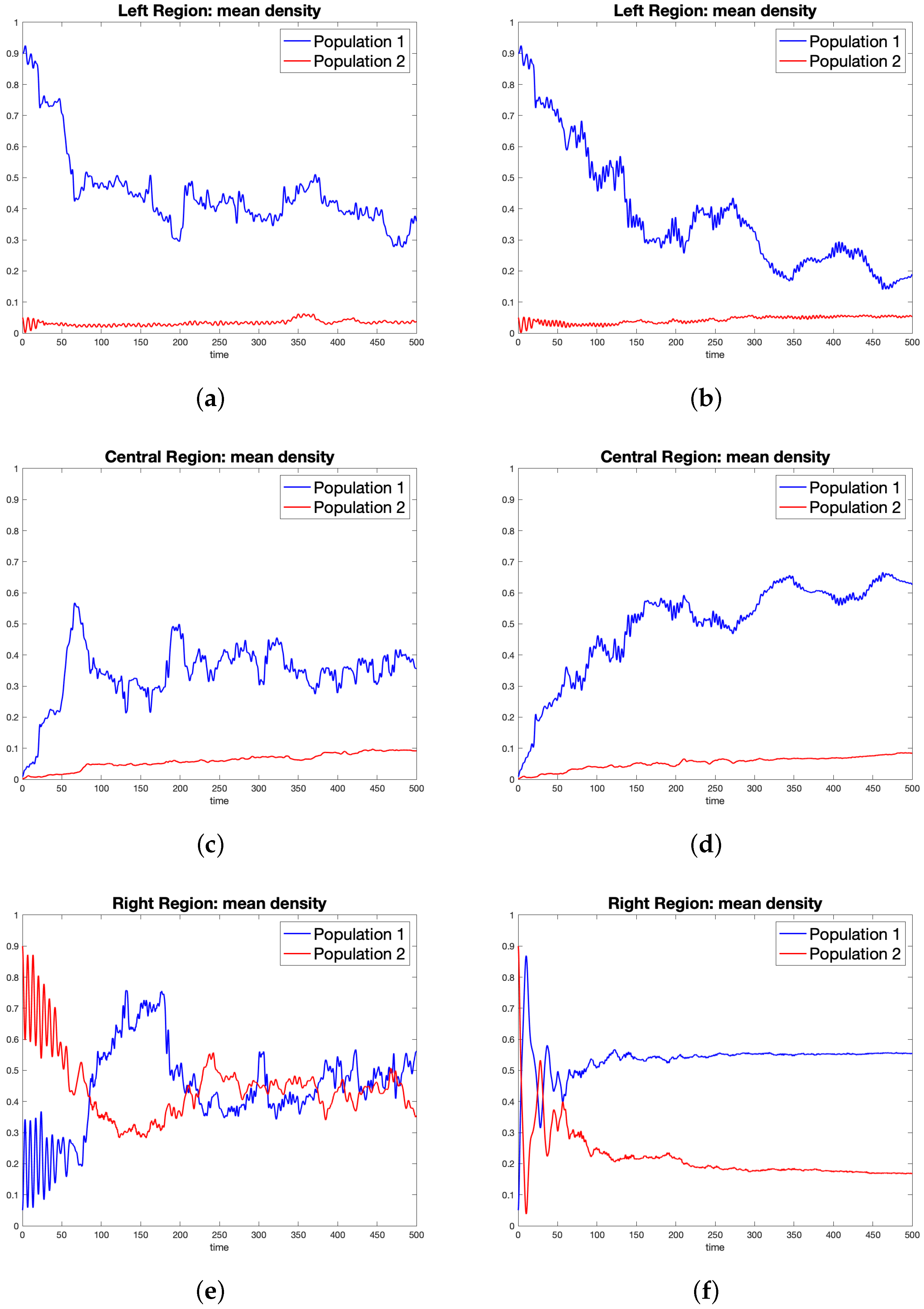
Each of the parameters entering the Hamiltonian is constant in each subregion; population $P_1$ possesses inertia parameters smaller than those of population ${\mathcal{P}}_2$, but greater mobility parameters $\mu$’s; the competitive interaction parameters in the first and third subregions are greater than those in the central subregion, and the nonlocal interaction is weaker than the local one. Moreover, the parameters responsible for competition (${\lambda }_{\alpha }$ and ${\nu }_{\alpha }$) are very small in the central region, and have their maximum in the right region. The concrete situation we want to describe is the following one. The left subregion ${\mathcal{C}}_1$ could be thought of as a poor region, the right subregion ${\mathcal{C}}_3$ as a rich region, and the central subregion ${\mathcal{C}}_2$ as the region that the poorer population ${\mathcal{P}}_1$ needs to cross with the aim of going to the richest subregion and improving its wealth. Such a situation is somehow similar to the one considered in [25], where a model including only local competition and migration (without any rule) has been investigated. As clearly shown in Figure 1b,d,f for the rule 1, the dynamical outcome is rather different if we take into account the $(\mathcal{H},\rho )$-induced dynamics approach.

Without the rules, the behavior of the local density in each cell is oscillatory, although the migration terms tend to make the densities uniform all over the three subregions. It is observed that both populations move to the right cells, and this effect is more evident for population ${\mathcal{P}}_1$ (Figure 1a,c,e); also, due to the structure of the Hamiltonian (and, consequently, to the quasiperiodic regime), the local densities do not definitely increase moving from the left to the right. On the contrary, a clear movement from left to right emerges when the rules are considered (Figure 1b,d,f for the rule 1). In the classical Heisenberg dynamics (no rule at all), population ${\mathcal{P}}_1$ tends to move towards the subregion ${\mathcal{C}}_3$: at least in the time interval $[0,200]$, the mean local density of ${\mathcal{P}}_1$ decreases in ${\mathcal{C}}_1$, and increases in ${\mathcal{C}}_2$ and ${\mathcal{C}}_3$. On the contrary, the mean local density of population ${\mathcal{P}}_2$ increases in ${\mathcal{C}}_1$, has a small variation in ${\mathcal{C}}_2$, and decreases in ${\mathcal{C}}_3$. Nevertheless, due to the quasiperiodic regime, this trend is not preserved for all times. Using rule 1 (Figure 1b,d,f), this movement of population ${\mathcal{P}}_1$ towards subregion ${\mathcal{C}}_3$ is much more evident than the movement of population ${\mathcal{P}}_2$, and this is reasonable because of the different mobility parameters. Here, it is worth of being remarked that, in the right region, the mean local densities of the two populations tend to approach a sort of equilibrium; moreover, there is also an inversion, in the sense that population ${\mathcal{P}}_1$ becomes more abundant than population ${\mathcal{P}}_2$ (this is due to the initial values of inertia parameters of the two populations: population ${\mathcal{P}}_1$ has a greater tendency to change with respect to population ${\mathcal{P}}_2$). The quasiperiodic regime of the classical Heisenberg dynamics is modified by the effect of the rule that introduces a sort of irreversibility in the evolution, even if the sum of the local densities of the two populations in all cells remains constant, that is, the rule preserves the existence of the first integral.

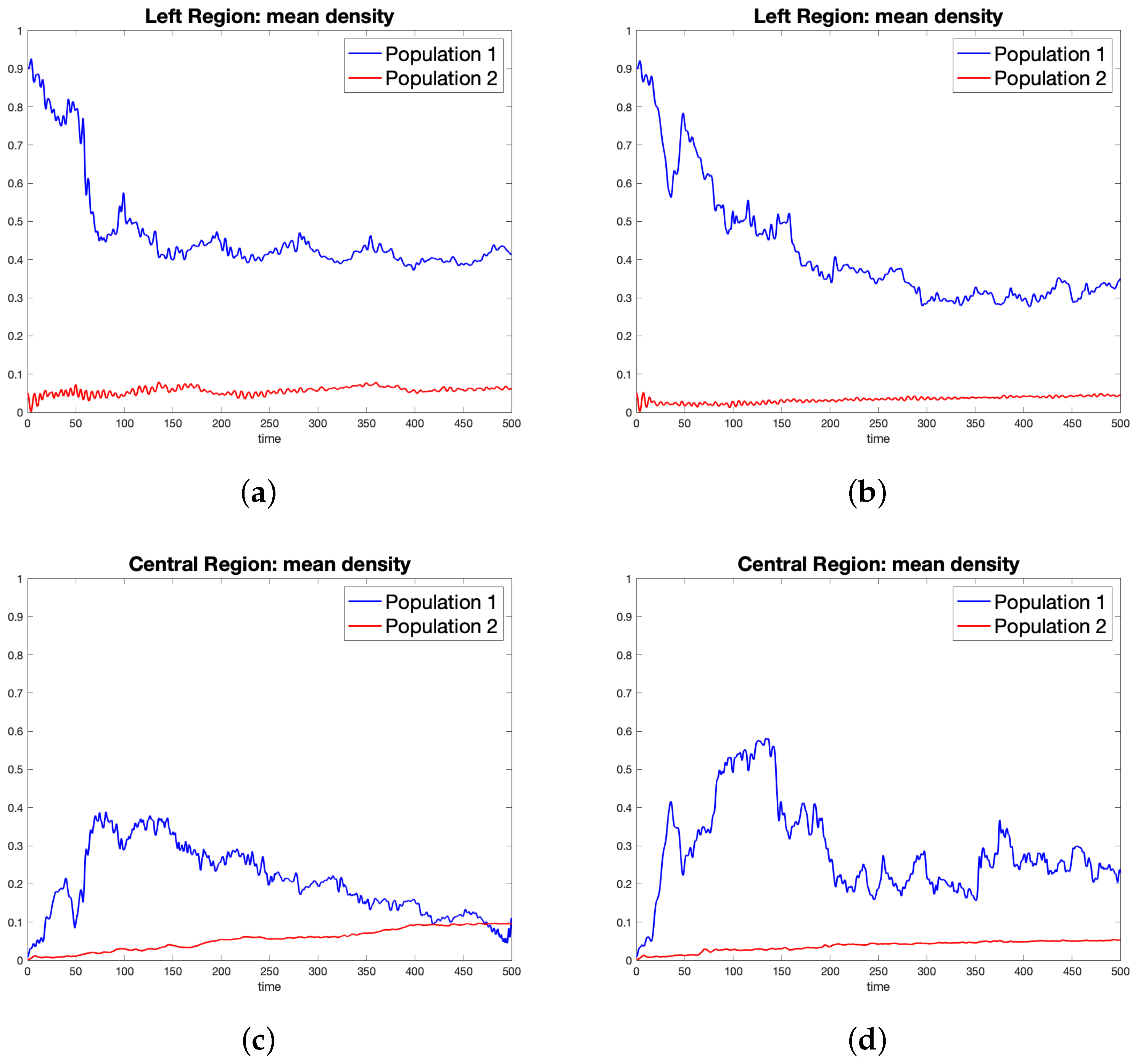
The same general considerations, though the dynamical outcomes are somehow different, apply also when the rules 2 and 3 are used. In fact, the effects of the rules 2 and 3 (one again with the choice $\tau =1$), that modify also the mobility parameters, are shown in Figure 2, where the migration of both populations towards the right cell has a more definite trend; moreover, it is observed that the amplitude of the oscillations of the mean densities in the three subregions decreases with time.

3.2. Second Scenario

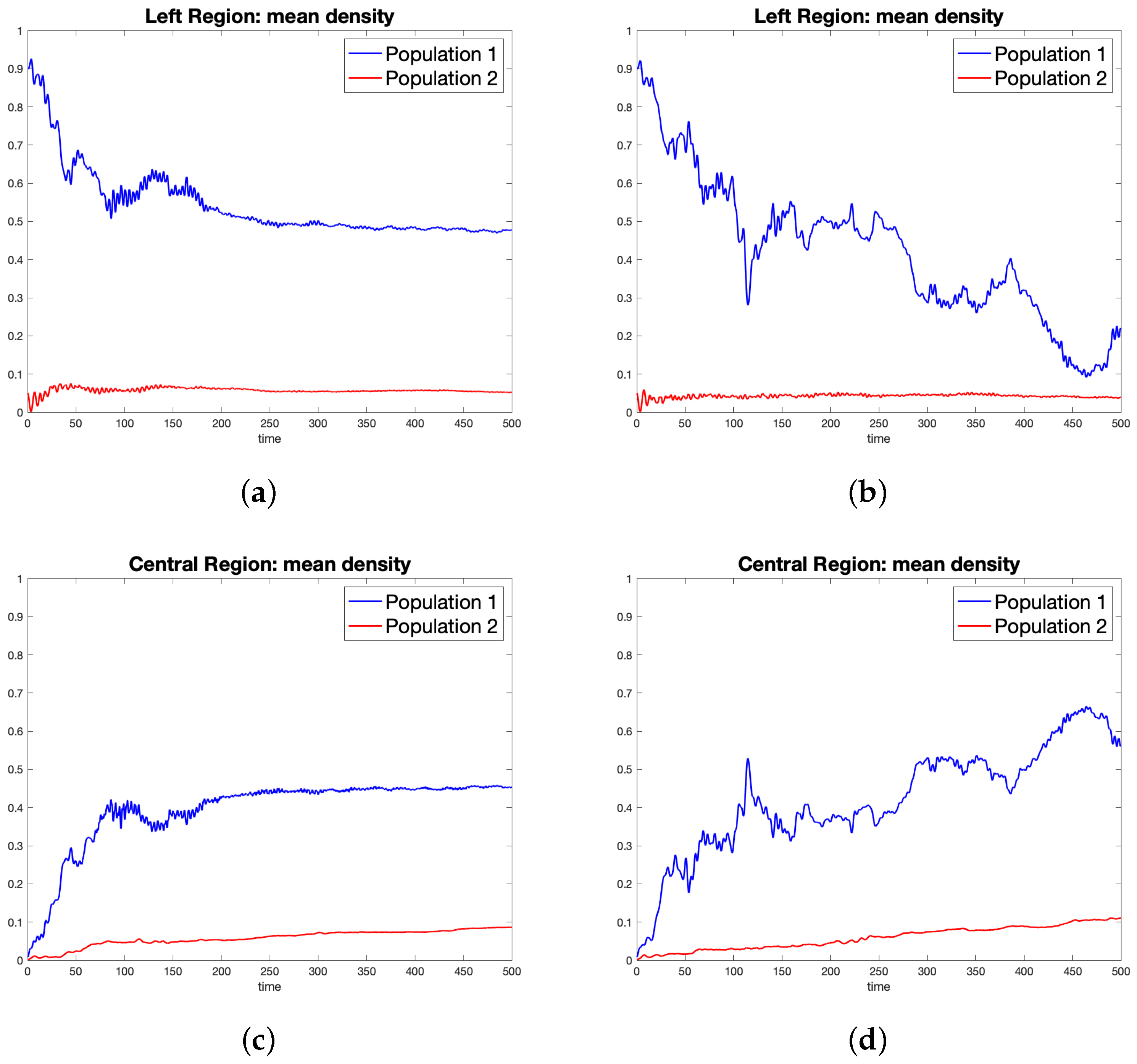
Here, the only difference with respect to the previous case is that the central region is not sparsely inhabited even if population ${\mathcal{P}}_1$ is more abundant than population ${\mathcal{P}}_2$; in some sense, the central subregion is not a transit area but a region with intermediate conditions of wealth.

We assume the following initial conditions:

$$\begin{array}{ccc}{n}_{1,\alpha }^0=0.9,\hfill & n_{2,\alpha }^0=0.05\hfill & \alpha \in {\mathcal{C}}_1,\hfill \\ n_{1,\alpha }^0=r_{\alpha }(0.3,0.5),\hfill & n_{2,\alpha }^0=r_{\alpha }(0.15,0.35)\hfill & \alpha \in {\mathcal{C}}_2,\hfill \\ n_{1,\alpha }^0=0.05,\hfill & n_{2,\alpha }^0=0.7\hfill & \alpha \in {\mathcal{C}}_3.\hfill \end{array}$$

(19)

As far as the choice of parameters is concerned, we choose

$$\begin{array}{cc}\hfill & {\omega }_{1,\alpha }=0.4,{\omega }_{2,\alpha }=0.7,\alpha \in \mathcal{C},\hfill \\ \hfill & {\lambda }_{\alpha }=\left\{\begin{array}{cc}0.05,\hfill & \alpha \in {\mathcal{C}}_1,\hfill \\ 0.01,\hfill & \alpha \in {\mathcal{C}}_2,\hfill \\ 0.1,\hfill & \alpha \in {\mathcal{C}}_3,\hfill \end{array}\right.{\nu }_{\alpha }=\frac{{\lambda }_{\alpha }}{2},\hfill \\ \hfill & {\mu }_{1,\alpha }=\left\{\begin{array}{cc}(0.3\alpha +1.1)/14,\hfill & \alpha \in {\mathcal{C}}_1,\hfill \\ 0.4,\hfill & \alpha \in {\mathcal{C}}_2,\hfill \\ (-0.3\alpha +5.9)/14,\hfill & \alpha \in {\mathcal{C}}_3,\hfill \end{array}\right.{\mu }_{2,\alpha }=\frac{{\mu }_{1,\alpha }}{20}.\hfill \end{array}$$

(20)

Similar considerations as above can be made also in the second scenario, and the effect of the rules (Figure 3b,d,f and Figure 4) is evident with respect to the outcomes of the classical Heisenberg dynamics.

3.3. The Role of $\tau$

In the $(\mathcal{H},\rho )$-induced dynamics approach, the choice of the value of $\tau$, that is, the length of the time interval after which some of the parameters entering the Hamiltonian are changed, has its influence on the time evolution. This is shown in Figure 5, Figure 6 and Figure 7 (for the first scenario), and Figure 8, Figure 9 and Figure 10 (for the second scenario).

4. Conclusions

In this paper, we constructed an operatorial model based on fermionic ladder operators to describe the dynamical behavior of two populations competing each other and able to diffuse in a one-dimensional spatial region made by a finite number of adjacent cells; the two populations compete locally (in the same cell) and nonlocally (in the adjacent cells). The mean values of the number operators associated with the two populations in a cell are interpreted as a measure of their local density in the cell. The dynamics is ruled by a self-adjoint and time-independent quadratic Hamiltonian operator; consequently, adopting the classical Heisenberg viewpoint, the dynamics is ruled by linear differential equations. To enrich the dynamics, we introduced some rules and used the recently introduced $(\mathcal{H},\rho )$-induced dynamics approach. Two different scenarios and three different sets of rules have been considered and the corresponding numerical results have been presented.

The dynamical outcomes show that this model is compatible with the coexistence of the two competing populations in the same environment. The model is susceptible of various extensions and generalizations. For instance, we may include in the Hamiltonian effects due to cooperative interactions between the two populations, as well as construct a spatial model in a two-dimensional region, thereby extending the results given in [25], where the approach of $(\mathcal{H},\rho )$-induced dynamics has not been used. Some of these extensions are currently planned and will be the subject of a forthcoming paper.