1. Introduction
Studies of the dynamics of systems possessing higher than geometric symmetry (also known algebraic symmetry, or hidden symmetry) have a great fundamental importance. This is because algebraic symmetry facilitates the possibility of analytical solutions for these systems. In turn, the analytical solutions offer a physical insight into the complicated dynamics of these systems—in distinction to simulations.
A more general concept is dynamical symmetries. For classical systems, a dynamical symmetry corresponds to the property of the system, such that there are transformations in the phase space that leave the dynamics of the system invariant. For quantum systems, a dynamical symmetry corresponds to the property of the system, such that there is a set of operators commuting with the Hamiltonian and, thus, these operators correspond to conserved quantities. If the number of such transformations for a classical system or the number of such operators for a quantum system is greater than the corresponding number resulting from a geometrical symmetry of the system (such as, e.g., the spherical or axial symmetry), the situation is described as the algebraic, or hidden, symmetry.
Hidden symmetries are important because they facilitate the separation and the integration of the equations of motion. The resulting analytical solutions allow a profound physical insight into the dynamics of such physical systems—an insight that is impossible to obtain by simulations.
In the first several chapters of this review, we present studies of the dynamics of different kinds of one-electron Rydberg quasimolecules (OERQ). We start from the configuration where an electron moves in the field of two stationary Coulomb centers (TCC) of charges
Z and
Z’, separated by a distance
R (diatomic Rydberg quasimolecules). Crossings and quasicrossings of the terms are exhibited by OERQ. This makes OERQ suitable for studying charge exchange, the latter being of practical importance (see, e.g., [
1,
2,
3,
4,
5,
6] and references therein).
The Neumann–Wigner general theorem denotes that terms of the same symmetry [
7] cannot cross. However, it does not apply to the TCC problem of
Z’
≠ Z—see, e.g., paper [
8]. This is because, for the TCC problem, it is possible to separate variables into elliptic coordinates [
8]. Specifically, there are two potential wells—one centered at the
Z charge, another centered at the problem of the
Z’ charge. They have states described by the same quantum numbers [
9,
10,
11]. Due to this degeneracy, there is a much higher probability for the electron to undergo tunneling from one well to another (in distinction to cases of no degeneracy). This means that charge exchange occurs at such quasicrossings.
In Oks’ book [
12], it was written:
“These rich features of the TCC problem also manifest in a different area of physics such as plasma spectroscopy as follows. A quasicrossing of the TCC terms, by enhancing charge exchange, can result in unusual structures (dips) in the spectral line profile emitted by a
Z-ion from a plasma consisting of both
Z- and
Z’-ions, as was shown theoretically and experimentally [
13,
14,
15,
16,
17,
18]. From the experimental width of these dips, it is possible to determine rate coefficients of charge exchange between multicharged ions, which is a fundamental reference data virtually inaccessible by other experimental methods”.
Before the year 2000, the paradigm was that the above sophisticated features of the TCC problem and its flourishing applications were inherently quantum phenomena. However, then, in the year 2000, papers [
19,
20] were published, presenting a purely classical description of both the crossings of energy levels in the TCC problem and the dips in the corresponding spectral line profiles caused by the crossing (via enhanced charge exchange). These classical results were obtained analytically based on first principles, without using any model assumptions.
In the classical studies, the TCC systems represent diatomic Rydberg quasimolecules encountered, e.g., in plasmas containing more than one kind of multicharged ion. Naturally, the classical approach is well suited for Rydberg quasimolecules.
It should be emphasized that, in the ground-breaking theoretical papers [
19,
20], analysis was not confined to circular orbits of the electron. Paper [
20] presented a detailed study of the
helical Rydberg states of these diatomic Rydberg quasimolecules. For stable motion, the electron trajectory was found to be a helix on the surface of a cone, with the axis coinciding with the internuclear axis. In this
helical state, the electron, while spiraling on the surface of the cone, oscillates between two end circles, which result from cutting the cone by two parallel planes perpendicular to its axis. In
Appendix A, we reiterate the basic results on the classical energy states of diatomic Rydberg quasimolecules.
In this review, first we present studies of the dynamics of diatomic Rydberg quasimolecules in various environments, such as being subjected to electric and/or magnetic fields or to a plasma environment. Then, we present the corresponding studies of other configurations, such as a one electron Rydberg quasimolecule that consists of a proton, an electron and a muon, and examine the integrals of motion in the TCC system. The higher than geometrical symmetry of these systems is due to the existence of an additional conserved quantity: the projection of the supergeneralized Runge–Lenz vector on the internuclear axis [
21]. The review also covers the dynamics of some muonic atoms exhibiting higher than geometric symmetry. Atomic units (
ħ =
e =
me = 1) are used throughout the whole study.
2. The Effect of a Static Electric Field on the Dynamics of One Electron Rydberg Quasimolecules: Enhancement of Charge Exchange and of Ionization
In papers [
18,
20,
21], the circular Rydberg states (CRS) of the TCC system were studied (in [
20] the analysis went beyond CRS). CRS of atomic and molecular systems with a single electron correspond to |
m| = (
n − 1) >> 1, with
n and
m being the principal and magnetic electronic quantum numbers, respectively. They have been studied profoundly [
22,
23,
24,
25], both theoretically and experimentally, for the reasons enumerated in Chapter 1.
In [
21], the effect of a magnetic field, directed along the internuclear axis, on CRS of the TCC system was studied analytically; in this chapter we study the effect of an electric field (also directed along the internuclear axis) on CRS of the TCC system. For strong fields, we obtained analytical results; for moderate fields, numerical results were obtained by using the standard software Mathematica. We found that the electric field causes the following changes. First, an extra energy term appears, which is not present in the zero field case—a fourth term, besides the three classical energy terms. Second, there appear additional crossings of the energy terms, which is a more important result. Some of these crossings enhance charge exchange, and other crossings enhance the ionization of the Rydberg quasimolecule.
2.1. The Classical Stark Effect for a Circular State of a Rydberg Quasimolecule
We study a TCC system, with the charge Z at the origin and the internuclear Oz-axis going from Z to charge Z’, which is at z = R, placed into a uniform electric field F antiparallel to the Oz-axis. We consider CRS where the electron has a circular orbit in the plane perpendicular to the Oz-axis, with the circle centered at this axis.
The energy
E and the projection of the angular momentum on the internuclear axis
L are conserved in this configuration. We write the equations for both quantities in cylindrical coordinates:
where (
ρ,
φ,
z) are the cylindrical coordinates of the electron, and
r and
r’ are the distances from the electron to charges
Z and
Z’, respectively.
The circularity of the electron orbit means that
dρ/dt = 0; also, because the orbit is perpendicular to the
z-axis,
dz/dt = 0. Then, we express
r and
r’ by means of
ρ and
z, and with
dφ/dt from (2), we obtain:
Using the scaled quantities
we give our energy equation the following form:
The equilibrium points can be found by setting the partial derivatives of the scaled energy (5) by the scaled coordinates
w and
v equal to zero. This yields the following two equations:
From (4), combining the last two equations, we have
ℓ2 = 1/
r. Then, we take the fourth and the last equations,
E = −(
Z/
R)
ε and
r =
ZR/
L2, which give
E = −(
Z/
L)
2 ε/
r, and the equation
r = 1/
ℓ2 can be obtained by solving (7) for
ℓ. After substituting
ℓ into the equation for the energy, we obtain the three equations—the master equations—for this configuration.
where, now, the energy in atomic units is expressed through the new scaled energy
ε1 as
E = −(
Z/
L)
2 ε1, and we introduce the notation
p =
v2. The new scaled energy
ε1 is, therefore, the “true” scaled energy, which enters the equation for
E without including
R. The quantities
ε1 and
r in (8) and (9) now have explicit dependence only on the scaled coordinates
w and
p for the given constants
b and
f. Therefore, by solving (10) for
p and substituting it into (8) and (9), we will obtain the parametric solution
ε1(
r), with the coordinate
w as the parameter.
We pay special attention to the crossings of energy terms of the
same symmetry. In the TCC problem in the quantum case, the notion “terms of the same symmetry” refers to terms of the same magnetic quantum number
m [
8,
9,
10,
11]. Thus, in our classical case of the TCC problem, we fix the quantity of
L and study the classical energy at
L = const ≥ 0 (because the cases of
L and −
L are the same, physically).
There is no exact analytical solution of (10) for p. We will use an analytical approximation.
In a contour plot (w, p) for a relatively weak field, f = 0.3, at the ratio b = 3, there are two branches in the plot: the left branch goes from w = 0 to w = w1 and the right branch has a small two valued region between some values: w = w3 and w = 1 (w3 < 1).
The right branch intersects the abscissa at
w = 1 and at a greater value:
w =
w2. We provide the analytical expressions for
w1 and
w2 in
Appendix B. The lower bound of the two-valued region
w3 is a solution of the equation
Appendix C shows the method to find
w3, as given in (11).
For the case of a relatively strong field, f = 20, at b = 3, the two-valued region vanishes.
Let us consider the case of a relatively small radius of the orbit of the electron, which corresponds to p << 1. This case corresponds physically to strong fields, f > fmin ~ 10.
Applying a small
p approximation to (10), we obtain the approximate solution
corresponding to the left branch (0 <
w <
w1) and
corresponding to the right branch (1 <
w <
w2). Substituting the solutions in (12) and (13) into (8) and (9), we obtain approximate analytical parametric solutions for the energy terms −
ε1(
r) for the regions of both branches, with the parameter
w.
We performed a numerical solution of the problem as well. Comparing it to the analytical solution, we found that the latter is accurate for fields f ≥ 5.
The electric field introduces the following changes compared to the zero field case. Compared to the case of f = 0, where three classical energy terms were found, the electric field generates the fourth energy term. There are four energy terms that we label as follows:
Term 2 is absent in the case of f = 0, but it appears at any non-zero value of f. As f approaches zero, this term behaves like −f/r, which is why it vanishes at f = 0.
The physical explanation for the appearance of the additional term is as follows. At
f = 0, there are no equilibrium points on the orbital plane to the right of
Z’ (i.e., for
w > 1), the limits
w1 and
w3 reduce to the ones given in [
19,
20], and the right branch of
p(
w) asymptotically goes to infinity when
w approaches
w3 from the right. When an infinitesimal electric field
f appears, the right branch of
p(
w) goes over positive infinity and ends up on the
w-axis at
w2 → ∞, enabling the whole region
w > 1 for equilibrium. As the field increases,
w2 decreases. What happens physically is that the force from the field at
w > 1 balances out the Coulomb attraction of the
Z–
Z’ system to the left of the electron—a situation not possible for
f = 0. This term is obtained by varying the parameter
w from 1 to
w2.
The above examples for Z’/Z = 3 represent a typical situation. In fact, for any pair of Z and Z’ ≠ Z, in the presence of an electric field, there are four classical energy terms of the same symmetry for CRS.
The electric field introduces another important feature, X type crossings of the energy terms. We discuss this type of crossings and their physical consequences in the next section.
2.2. X Type Crossings of Classical Energy Terms
Term 2 has an X type crossing with term 3 at r = 7.8 and an X type crossing with term 4 at r = 32. Two X type crossings are observed for a limited range of the electric field. Particularly, for b = 3:
two X type crossings at 1.31 < f < 2.4;
no X type crossings at f < 1.31;
one X type crossing at f > 2.4 (the crossing of terms 2 and 3).
To reveal the physical nature of the X type crossings, we will discuss the origin of all the four energy terms for an arbitrary b = Z’/Z ≠ 1, considering each term in the asymptotic limit r → ∞.
Term 3 corresponds to the energy of a hydrogen-like ion of nuclear charge
Zmin = min(
Z’,
Z), slightly perturbed by the charge
Zmax = max(
Z’,
Z) [
19,
20].
Term 4 corresponds to a near zero energy state (where the electron is almost free) [
19,
20]. If
b =
Z’/
Z is of the order of (but not equal to) unity, this term can be described only in elliptical coordinates (rather than parabolic or spherical coordinates), which means that, even at the asymptotic limit
r → ∞, the electron is shared by the
Z and
Z’ centers. However, in the case of
Z’ >>
Z, this term can be asymptotically considered as the
Z’ term [
19,
20]. It has a V type crossing with term 3, which is asymptotically the
Z term (since
Zmin =
Z for
Z’ >
Z). Similarly, in the case of
Z’ <<
Z, term 4 can be asymptotically considered as the
Z term [
19,
20]. It has a V type crossing with term 3, which asymptotically is the
Z’ term (since
Zmin =
Z’ for
Z’ <
Z).
Term 1 corresponds to the energy of a hydrogen-like ion of the nuclear charge
Zmax, slightly perturbed by the charge
Zmin [
19,
20].
Term 2 has properties similar to term 4, but with Zmax and Zmin interchanged. Particularly, in the case of Z’ >> Z, this term, at the limit, r → ∞ can be considered as the Z term, having a V type crossing with term 1, which, at the limit, is the Z’ term (since Zmax = Z’ for Z’ > Z). In the case of Z’ << Z, term 2 can be considered as the Z’ term, which has a V type crossing with term 1, which, at the limit, is the Z term (because Zmax = Z for Z’ < Z).
Thus, in case of a significant difference between
Z and
Z’, we observe the V type crossings of two terms that can be asymptotically labeled as
Z and
Z’ terms. This situation
corresponds classically to charge exchange [
19,
20]. We shall look at it in more detail: initially, at the limit
r → ∞, the electron was part of the
Zmin ion. As
Z and
Z’ move relatively close to each other, the two terms undergo a V type crossing and the electron is shared by both
Z and
Z’ centers. Then, as
Z and
Z’ move away from each other, the electron ends up as part of the
Zmax ion.
Thus, one of the changes brought by the electric field is an additional, second, V type crossing between terms 1 and 2 (which we denote as V12) leading to charge exchange, whereas, in the absence of the electric field, there was only one V type crossing—the one between terms 3 and 4 (which we denote as V34). However, V12 occurs at the internuclear distance rV12 << rV34, where rV34 is the internuclear distance of V34. Therefore, the cross-section of the charge exchange due to V12 is much smaller than the corresponding cross-section due to V34.
Now we will discuss the X type crossing in a similar way. With a significant difference between Z and Z’, the X type crossing of terms 2 and 4 (denoted as X24) is the crossing of terms that are asymptotically Z- and Z’-terms. Thus, this situation again corresponds classically to charge exchange. The most important here is that X24 occurs at a much greater internuclear distance: rX24 >> rV34 >> rV12. Therefore, the cross-section of the charge exchange corresponding to X24 is much greater than the cross-sections due to the V type crossings. This is the most fundamental physical consequence caused by the electric field: a significant enhancement of charge exchange.
With a significant difference between
Z and
Z’, the X type crossing of terms 2 and 3 (denoted as X23) is the crossing of terms with the same asymptotic labeling: both of them are
Z terms or
Z’ terms. Therefore, X23 (at
r =
rX23) does not correspond to charge exchange—rather, it represents an
additional ionization channel. In more detail, let us consider as an example that, initially, at the limit
r → ∞, the electron resided on term 3 of the
Z ion. As the distance between the charges
Z and
Z’ decreases to
r =
rX23, the electron can switch to term 2, which, at the limit
r → ∞, corresponds to a near zero energy state of the same ion
Z, where the electron would be almost free, which means that (as the authors wrote in [
26]) “as the charges
Z and
Z’ go away from each other, the system undergoes ionization. Thus, another physical consequence caused by the electric field is the appearance of the additional ionization channel. This should have been expected since the electric field promotes the ionization of atomic and molecular systems.”
2.3. Conclusions
We studied the effect of an electric field antiparallel to the internuclear axis on circular Rydberg states of the two Coulomb center system. We obtained (as the authors wrote in [
26]) “analytical results for strong fields and numerical results for moderate fields. We found that the electric field caused the following effects”.
The first effect is the appearance of an extra energy term: the
fourth classical energy term—besides the three classical energy terms at the absence of the field. As the authors wrote in [
26], “this term exhibits a V-type crossing with the lowest energy term. The two highest energy terms continue having a V-type crossing, like at the zero field”. When the charges
Z and
Z’ are significantly different, both V type crossings correspond to a charge exchange.
As the authors wrote in [
26], “the second effect is the appearance of a new type of crossing: X-type crossings. One of the X-type crossings (existing in a limited range of the electric field strength) corresponds to charge exchange at a much larger internuclear distance than the V-type crossings. Therefore the cross-section of charge exchange due to this X-type crossing is much greater than the cross-section of charge exchange due to V-type crossings. Thus, the electric field can
significantly enhance charge exchange.” We consider this to be the most important result of the present chapter.
The other X type crossing does not correspond to charge exchange: it represents an additional ionization channel.
3. The Effect of Plasma Screening on the Dynamics of the Circular States of Diatomic Rydberg Quasimolecules and Their Application to Continuum Lowering in Plasmas
In the previous chapters we studied analytically CRS of the two Coulomb center system, the system (denoted as
ZeZ’) consisting of two nuclei of charges
Z and
Z’, separated by a distance
R, and an electron—see also [
19,
20,
21,
26,
27,
28,
29]. Energy terms of these Rydberg quasimolecules were obtained for a case without a field, with an electric field and with a magnetic field.
The Rydberg quasimolecules of this type are naturally encountered in high density plasmas of several types of ions, where a fully stripped ion of charge Z’ is in the proximity of a hydrogen-like ion of nuclear charge Z (or where a fully stripped ion of charge Z is in the proximity of a hydrogen-like ion of nuclear charge Z’). Therefore, in the present chapter, we study the effects of plasma screening on CRS of these Rydberg quasimolecules—the effects not taken into account in the previous works. We obtain analytical results for weak screening and numerical results for moderate and strong screening. We show that the screening introduces the following effects.
The screening causes an additional energy term to appear—compared to the absence of the screening. This new term has a V type crossing with the lowest energy term. The internuclear potential is also affected by the screening, destabilizing the nuclear motion for Z > 1 and stabilizing it for Z = 1.
We also study the effect of plasma screening on continuum lowering (CL) in the ionization channel. As the authors wrote in [
30], “CL has been studied for more than 50 years—see, e.g., books/reviews [
31,
32,
33,
34,
35] and references therein. Calculations of CL evolved from ion sphere models to dicenter models of the plasma state [
33,
36,
37,
38,
39,
40,
41]. One of such theories—a percolation theory [
33,
38]—calculated CL defined as an absolute value of the energy at which an electron becomes bound to a macroscopic portion of plasma ions (a quasi-ionization). In 2001 one of us derived analytically the value of CL in the true-ionization channel which was disregarded in the percolation theory: a quasimolecule, consisting of the two ion centres plus an electron, can get ionized in a true sense of this word before the electron would be shared by more than two ions [
42]. […] It was also shown in [
42] that, whether the electron is bound primarily by the smaller or by the larger out of the two positive charges
Z and
Z’, makes a dramatic qualitative and quantitative difference for this ionization channel.” The results in [
42] were obtained for circular states of the Rydberg quasimolecules.
In the present chapter, we show that the screening decreases CL in the ionization channel, making CL vanish as the screening factor increases.
3.1. The Effect of Plasma Screening and Classical Energy Terms for a Rydberg Quasimolecule in a Circular State
As the authors wrote in [
30], plasma screening of a test charge is a well-known phenomenon. For a hydrogen atom or a hydrogen-like ion, it is equivalent to replacing the Coulomb potential with a screened Coulomb potential, which contains a physical parameter—the screening length
a. For example, the Debye–Hückel (or Debye) interaction of an electron with an electronic shielded field of an ion of charge
Z, is
U(
R) = –(
Ze2/
R)exp(–
R/
a), where
a = (
kT/(4π
e2Ne))
1/2 ≈ 6.90(
T/
Ne)
1/2, where
Ne (cm
−3) and
T (K) are the electron density and temperature, respectively.
In this chapter, we consider a two Coulomb center (TCC) system with charge Z placed at the origin, and the z-axis directed at the charge Z’, which is at z = R; this system is submerged in a plasma of screening length a. We consider the circular orbits of the electron that are perpendicular to the internuclear axis (z-axis) and centered on this axis.
Two quantities, the energy,
E, and the projection of the angular momentum on the internuclear axis,
L, are conserved in this configuration. Using cylindrical coordinates, we write the equations for both:
where
r and
r’ are distances from the electron to
Z and
Z’. The circular motion means that
dρ/dt = 0, and, as the plane of the orbit is perpendicular to the
z-axis,
dz/dt = 0. We express
r and
r’ through
ρ and
z, and take
dφ/dt from (15), obtaining the following expression for the energy:
With the scaled quantities
we give the energy Equation (16) the following form:
At the equilibrium points, the partial derivatives of
ε by the scaled coordinates
w,
p vanish. This yields the following two equations:
Here, we perform the steps to obtain the master equations for the energy terms, as we did in the previous chapter. From (17),
ℓ2 = 1/
r,
E = −(
Z/
R)
ε and
r =
ZR/
L2, so
E = −(
Z/
L)
2 ε/
r, where
r = 1/
ℓ2 is obtained by solving (20) for
ℓ. Thus,
ε/
r is the scaled energy without explicit dependence on
R, which we denote as
ε1. Thus, from (18)–(20), we derive the following three master equations for this configuration:
The quantities ε1 and r now explicitly depend only on the coordinates w and p (besides the constant screening parameter λ). Therefore, resolving (23) for p and substituting it to (21) and (22), we obtain the parametric solution for the energy terms ε1(r), with the parameter w varied over the allowed range, for the given quantities b and λ.
Equation (23), which represents the equilibrium points on the (w, p) plane, cannot be solved analytically for p. Therefore, we will make an analytical approximation.
As in [
20] and Chapter 2, the corresponding plot has two branches, the left one from
w = 0 to
w =
w1, and the right one from the asymptote
w =
w3 to
w = 1. Moreover,
w1 is a solution of the equation
in the interval 0 <
w1 < 1, and
w3 does not depend on λ and equals
b/(1 +
b)—the same as in [
20] for λ = 0, the “default” case described in Chapter 1. As λ increases,
w1 and the
p coordinate of the maximum of the left branch increase, but the general shape of both curves is preserved. Below is the plot for a relatively strong λ = 2.
We made an approximation for small values of λ. Approximating (23) in the first power of λ, we obtain the expression involving only the second and higher powers of λ. Therefore, an attempt was made using the value of
p(
w) for λ = 0 presented in [
20] and in (A5), which we shall denote as
p0. Further, taking into account the higher powers of λ, we obtained the next order approximation for
p(
w):
where
which is the zero-λ value, as in (A5).
We can approximate (24) by substituting 1 + λ(1 − 2
w1) in place of exp(λ(1 − 2
w1)), which will render it a 4th degree polynomial in
w1. The analytical expression for it is given in
Appendix D.
Substituting (25) into (21) and (22), we obtain the approximate parametric solution for the energy terms −
ε1(
r) by running the parameter
w on 0 <
w <
w1 and
w3 <
w < 1. Empirically, by comparison with the numerical results, it was found that using the value of
p from (26) on the 0 <
w <
w1 range and from (25) on the
w3 <
w < 1 range, gives the best approximate results.
Figure 1 presents the approximate terms for
b = 3 and different values of λ.
We also completed a numerical solution by solving (23) numerically for
p and substituting it into (21) and (22). This shows that the analytical solution is a good approximation for λ < 0.3.
Figure 2 presents the terms plotted for selected values of λ.
We should remind the reader of the following. These plots show “classical energy terms” of the same symmetry. (In the treatment of diatomic molecules, the expression “energy terms of the same symmetry” means the energy terms corresponding to the same component of the angular momentum L on the internuclear axis.) For the given values of internuclear distance R and angular momentum L, the classical energy E has only several discrete values. However, when L assumes a continuous set of values, so does E (as it should be in classical physics).
3.2. Crossings of the Energy Terms
We have studied the following properties of the energy terms. For small or moderate λ, there are four terms, with both pairs having a V type crossing. As an example, we take the plot of the terms for the case of λ = 0.2 (the red curve in
Figure 1 and the blue curve on
Figure 2) and number the lowest term 1 and the highest term 2; we number the remaining terms 3 and 4, from the lower one to the higher one, as in Chapter 2. Thus, the pair “terms 1 and 2” and the pair “terms 3 and 4” have a V type crossing each; we shall refer to these crossings as V12 and V34. Using a zero λ approximation by choosing (26) as the
p(
w) solution for the energy terms, we can substitute (26) into (22), which will give it the form below.
For a given value of
b, terms 3 and 4 are produced by varying
w over the range 0 <
w <
w1. The V34 crossing occurs at the value of
w where
r(
w) is at its minimum [
20]. Thus, solving
dr/
dw = 0, we obtain the equation whose solution for
w in the range 0 <
w <
w1 gives us the point on the parametric axis that produces the V34 crossing.
As this is for the case λ = 0, it is equivalent to the Coulomb potential case studied in Chapter 1. Therefore, (28) has an analytical solution, shown in (A13), with the parameter
γ defined in (A10); so, the analytical solution of (28) in terms of
w has the following form:
We substitute solution (29) into (22) and, using the numerical solution for p(w) from (23), we obtain the semi-analytical dependence of the scaled internuclear distance rV34(λ), corresponding to the V34 crossing, on the screening parameter λ, for a given b.
We can obtain the energy −εV34(λ) corresponding to the V34 crossing semi-analytically by substituting the numerical solution for p of (23) into the expression for the energy in (21), and, further, by substituting the zero λ solution (29) into the resulting expression. We see that, as λ increases, the energy of the V34 crossing increases and, at a relatively large λ, becomes positive. As in the case of rV34(λ), we compared the semi-analytical and numerical plots for −εV34(λ), and found a good similarity between them.
As λ increases, the energy corresponding to the V34 crossing becomes positive after λ = 2.96 reaches its maximum and, then, asymptotically approaches zero. For b = 4/3, the V34 crossing reaches zero energy at λ = 2.13.
The shape of terms 3 and 4 also changes under the screening. Term 3, whose energy increases as
r increases for small λ, at a certain value of λ becomes nearly constant, with energy equal to −0.5; at greater λ, its energy decreases with
r. For
b = 3, this value of λ is about 1; for
b = 4/3, it is about 2/3.
Figure 3 and
Figure 4 present the plots.
For the V12 crossing, the small λ approximation does not apply because this crossing is not observed at λ = 0. Therefore, we used only numerical methods. A situation of particular interest is the behavior of term 1 at very small
r, because as
r → 0 it corresponds to the energy of the hydrogenic ion of the nuclear charge
Z +
Z’ [
27]. The point with the smallest
r corresponds to the V12 crossing. We made a comparison of the dependence of the energy of the electron on λ from [
27] and the limiting case
r → 0 in our situation. Since, in the paper mentioned above, the calculation was performed for a single Coulomb center
Z, we rescaled the quantities to make a valid comparison. The relation between the electronic energies in both cases is
ε1(TCC) = (1 +
b)
2ε1(OCC), where OCC stands for “one Coulomb center”. Since the scaling for the screening parameter in the OCC case did not include
R (the internuclear distance in the TCC case), the scaling factor in the relationship between the screening parameters in both cases includes
r: λ
(TCC) =
r(1 +
b)λ
(OCC).
3.3. The Effect of the Plasma Screening on the Internuclear Potential
We also studied the effect of the screening on the internuclear potential. Previously, internuclear potential properties were studied for the same system, with λ = 0 subjected to a magnetic field parallel to the internuclear axis [
21]. One of the results was that the magnetic field created a deep minimum in the internuclear potential, which caused the stabilization of the nuclear motion and transformation of a Rydberg quasimolecule into a real molecule. Here, we study the effect of the screening on the internuclear potential. The expression for the internuclear potential in atomic units is
where
E is the electronic energy. With the scaled quantities from (17), it takes the following form:
where
Uint = (
Z/
L)
2uint. From the plot of the dependence
uint(
r), we found that, for
Z > 1, the screening flattens the minimum, producing a destabilizing effect, opposite to the one of the magnetic field. In
Figure 5, we present the plots of
uint(
r) for the case of
Z = 2,
b = 2, λ = 0 and λ = 0.3.
With the screening, the potential corresponding to the intersection point of the two branches increases, and the upper branch, which has a very shallow minimum at λ = 0, loses this minimum as λ increases.
3.4. The Effect of the Plasma Screening on the Continuum Lowering
The results of our analysis of the stability of the motion of the electron are similar to the ones obtained before [
19,
20]. Particularly, term 3 corresponds to a stable motion, while term 4 corresponds to an unstable motion. Thus,
the V34 crossing point corresponds to the transition from stable to unstable motion, bringing the electron to a zero energy state (i.e., to free motion) along term 4—in other words, to the ionization of the molecule.
Therefore, we have the following situation. To ionize the hydrogen-like ion of the nuclear charge Zmin perturbed by the charge Zmax, it is enough to reach the scaled energy εc(b) = ε(wV34(b), b) < 0. At the V34 point, the electron switches to the term corresponding to unstable motion and the radius of its orbit increases without a limit. This means that the amount of CL is Z‹1/R›|ε(wV34(b), b)|, where ‹1/R› is the inverse distance of the closest neighboring ion from the radiating ion averaged over the perturbing ions.
In
Appendix E and
Appendix F we present the effects of the electric and magnetic fields on CL. We found that the magnetic field decreases the value of CL, similar to the case above, while the electric field increases the value of CL, promoting ionization.
3.5. Conclusions
We studied the effects of plasma screening on the classical energy terms of the electron in the field of two Coulomb centers. We provided analytical results for the small values of the screening factor and numerical results for the medium values.
We found that plasma screening leads to the appearance of a fourth energy term—besides the three classical energy terms that exist with no screening. This term has a V type crossing with the lowest term. The two other energy terms have a V type crossing, as in the case without plasma screening.
We studied the effect of the screening on the internuclear potential. We found that the nuclear motion was stabilized by screening for Z = 1 and destabilized for Z > 1.
The effect of the screening on the continuum lowering was studied as well. The plasma screening decreases the value of CL in the ionization channel, similar to the effect of the magnetic field [
21].
4. Dynamics of Helical and Circular States of Diatomic Rydberg Quasimolecules in a Laser Field
In the previous works [
19,
20,
21,
26,
27,
28,
43] and the previous chapters, there were presented analytical studies of two Coulomb center systems consisting of two nuclei of charges
Z and
Z’ separated by a distance
R and one electron, the system being in a circular Rydberg state. Classical energy terms of such systems for a field free case [
19,
20] were obtained, as well as in a constant electric field ([
26] and Chapter 2) or constant magnetic field [
21], and crossings of the energy terms were studied—those crossings in these systems that enhance charge exchange.
The analysis was not limited by the case of circular orbits of the electron. For instance, [
20] profoundly studied
helical states of such Rydberg quasimolecules. To present those results in a clearer way, we briefly enumerate here the steps of that analysis. Using the axial symmetry of the system, cylindrical coordinates (
z,
ρ,
φ) are introduced with the internuclear axis along the
z-axis and the
z and
ρ motions are separated from the
φ motion. Then, the
φ motion is found from the
ρ motion calculated previously. Then, the equilibrium points of the two dimensional motion in the
zρ space are studied, and the condition is found that distinguishes two physically different cases: where the effective potential energy in the
zρ space either has a two dimensional minimum or has a saddle point. Particularly, it was found that the boundary between these two cases corresponds to the crossing of the upper and middle energy terms (out of the three terms existing for this system in an unperturbed case). In the case of stable motion, it was found that the trajectory is a helix on the surface of a cone, with the axis of the cone coinciding with the internuclear axis. In this
helical state, the electron is spiraling on the surface of the cone and oscillating between the two limiting circles, which are intersections of the cone with two parallel planes perpendicular to the axis of the cone.
In the present chapter, we study such systems under a laser field. We note that, in this chapter, we consider the system whose
φ motion has a much larger frequency than the laser frequency, the latter being of the order of other characteristic frequencies in the
zρ-space—as opposed to Chapter 6, where the laser frequency is much greater than any other frequency of the system. In the case of the polarization of the laser field being linear along the internuclear axis, as the authors wrote in [
44], “we found an analytical solution for the stable helical motion of the electron valid for wide ranges of the laser field strength and frequency. […] We also found resonances, corresponding to a laser-induced unstable motion of the electron, that result in the destruction of the helical states”. In the cases with such systems being under a circularly polarized laser field, as the authors wrote in [
44], with the “polarization plane being perpendicular to the internuclear axis, we found an analytical solution for circular Rydberg states valid for wide ranges of the laser field strength and frequency. We showed that under the laser field with both cases of polarization, in the electron radiation spectrum, besides the primary spectral component at (or near) the unperturbed frequency” of the electron, satellites appear. We found that, in the case of linear polarization of the laser field, as the authors wrote in [
44], “the intensities of the satellites are proportional to the squares of the Bessel functions”
Jq2(
s), (
q = 1, 2, 3, …), with
s being proportional to the laser field strength. As for the case of the circular polarization of the laser field, we showed, as the authors wrote in [
44], “that there is a red shift of the primary spectral component, which is linearly proportional to the laser field strength.”
4.1. Analytical Solution for the Linear Polarization Case of a Laser Field
We study the case where the laser field is polarized parallel to the internuclear axis and undergoes sinusoidal oscillations with frequency
ω. The angular momentum
L of the electron is conserved here because of the azimuthal symmetry. The Hamiltonian in this case is
The frequencies are scaled by the factor (
R3/
Z)
1/2: for example, the scaled frequency of the laser field is
μ =
ω(
R3/
Z)
1/2. We use the coordinates scaled by the internuclear distance
R, as in [
19,
20] and the other chapters:
The origin of the coordinate system is at charge Z.
In the absence of the electric field, in the neighborhood of the equilibrium the
zρ motion is a two dimensional harmonic oscillator [
20]. Its scaled eigenfrequencies are
where
v is the equilibrium value given also in (A5) and in [
19,
20]:
The motion takes place on the axes (
w’,
v’), which are the axes (
w,
v) rotated by angle α [
20]. The dependence of α on
w can be expressed in a compact form by using the substitution presented in (A10):
In the
γ representation, it has the form
The scaled eigenfrequencies ω− and ω+ given in (34) are the scaled frequencies of small oscillations around the equilibrium along the coordinates w’, v’, accordingly.
When the oscillating electric field is introduced, these oscillations become driven, with the forces
F cos α cos
ωt along the coordinate
w’ and
F sin α cos
ωt along the coordinate
v’. Therefore, the deviations from equilibrium on (
w’,
v’) are (see, e.g., textbooks [
45,
46])
where
μ =
ω(
R3/
Z)
1/2 is the scaled laser frequency and
τ =
t(
Z/
R3)
1/2 is scaled time. Now, we switch back to the coordinates (
w,
v) and obtain the equations of motion in the oscillating electric field with linear polarization in the neighborhood of the equilibrium: the electron moves around the circular path defined by the zero field case, with deviations from equilibrium depending on the scaled time
τ:
Thus, the amplitudes of the driven oscillations (at the laser field frequency) in both directions are controlled by the frequency and the strength of the laser field.
The coordinate
φ in the Hamiltonian (32) is cyclic, so the canonical momentum
pφ is conserved:
We can rewrite (40) in terms of the scaled quantities:
where
ℓ =
L/(
ZR)
1/2 is the scaled angular momentum. Representing the
v coordinate as a sum of the equilibrium value (35) (denoted as
v0) and the deviation from the equilibrium (39),
v(
τ) =
v0 + δ
v(
τ), we substitute it in (41) and obtain
and, after integrating it by time, we obtain the
φ motion:
From (43), we see that the φ motion is a rotation around the internuclear axis with the scaled frequency ℓ/v02 slightly modulated by the oscillations of the scaled orbit radius v at the scaled laser frequency μ (i.e., at the laser frequency ω in atomic units).
Thus, from (39) and (43) it follows that the electron is constrained to a conical surface that incorporates the circular orbit corresponding to the zero field case.
We substitute the expression for
φ(
τ) from (43), i.e.,
φ(
t(
Z/
R3)
1/2), into the following Fourier transform to find the amplitude of the power spectrum of the electron radiation,
where Δ is the radiation frequency measured, e.g., by a spectrometer. The sinusoidal modulation of the phase
φ is analogous to the case of hydrogen spectral lines being modified by an external monochromatic field at the frequency
ω; the latter case was solved analytically by Blochinzew as early as 1933 [
47] (a further study can be found, e.g., in book [
48]).
We apply Blochinzew’s results to our case of an electron radiation spectrum, and we find that this helical motion should manifest in the following way. The emission with the most intensity would be at the frequency
Ω =
dφ/
dt of the rapid
φ motion. Additionally, there will appear satellites at the frequencies
Ω ±
qω, where
q = 1, 2, 3, …, whose relative intensities
Iq are given by the Bessel functions
Jq(
s):
The electron also oscillates in the zρ space with the laser frequency ω, so it should also cause radiation at this frequency. However, due to the fact that ω << Ω, this spectral component would be very distant from the primary spectral line and its satellites.
From (39), we also see that, when the laser frequency is equal to one of the eigenfrequencies of the motion in the zρ space (μ = ω+ or μ = ω−), there are resonances. We found that these conditions provide three resonance points on the internuclear axis (w-axis) for the laser field frequency μ below a certain critical value μc, or five resonance points for μ > μc.
For example, in the case of b = 3, for μ = 8, resonances are observed at the following five values of w: 0.02883, 0.1106, 0.2497, 0.9852, 0.9878. The critical value of the laser frequency corresponds to the minimum of ω+(w) for a given b in the interval 0 < w < w1, which can be found by calculating a derivative and equating it to zero. The value of ω+ at the minimum is equal to the critical value of the laser frequency μc. Particularly, for the case of b = 3, the minimum of ω+ is at w = 0.17642, and this critical value is μc = 7.5944. As b increases, the critical value μc increases.
These resonances result in a laser induced unstable motion of the electron and the destruction of the helical states. For a resonance case where b = 3, f = 1, μ = 8, and w = 0.111 (w = 0.111 is one of the three values of w at which the laser frequency μ coincides with the eigenfrequency ω+), the three dimensional trajectory of the electron (for various directions of its initial velocity) is strikingly distinct from the case of the stable helical motion: the resonance destroys the helical state.
4.2. Analytical Solution for the Circular Polarization Case of a Laser Field
Now we move on to the case of a circularly polarized laser field, where the polarization plane is orthogonal to the internuclear axis. Therefore, the laser field is given by the following expression:
where
ex and
ey are the unit vectors of the
x- and
y-axis,
F is the amplitude, and
ω is the frequency of the field. For this case, the electron will have the following Hamiltonian:
where we introduced
φ0 =
ωt. In the same way as in [
20], the
φ motion will be the rapid subsystem, i.e.,
dφ/
dt is much greater than
ω and the frequencies of
z and
ρ motion. From (47), we obtain the Hamilton equations for the
φ motion:
Substituting
pφ from (48) into (49), we have
Now we substitute
φ −
φ0 =
θ + π into (50):
which describes the motion of a mathematical pendulum of length
ρ in gravity
F. Its modes of motion are libration and rotation; because
θ is rapid, our case corresponds to rotation. The solution of (51) is well known and can be expressed in terms of the Jacobi amplitude:
In (52), we defined Ω = dθ/dt at t = 0. For rapid rotations, the angular speed of θ changes insignificantly compared to the initial angular speed, so dθ/dt ≈ Ω.
Expression (52) for
θ(
t) enters the Fourier transform that determines the amplitude of the power spectrum of the electron radiation:
We can calculate analytically the red shift of the primary spectral component. As the
φ motion is rapid, we can take the time average of the Hamiltonian in (47) in the following way. First, we integrate (51) with the initial condition
dθ/
dt =
Ω and obtain
Then, we average this equation with respect to time:
Thus, the time averaged
φ momentum term in the Hamiltonian (47) is
The time average of the last term in the Hamiltonian (47) is zero, so the time averaged Hamiltonian depends only on
ρ and
z coordinates and their corresponding momenta. Thus, the result of the time-averaging of (47) is the following quasistationary Hamiltonian with no explicit time dependence:
Introducing the following scaled quantities
and applying the Hamilton equations to (57), we obtain the following two differential equations of motion:
(the dot above the variable is differentiation by the scaled time
τ =
t(
Z/
R3)
1/2).
In this section, we consider circular, not helical, states of the Rydberg quasimolecules, so the plane of the electron orbit is stationary with respect to the internuclear axis. This makes the right hand side of (59) vanish, yielding the same (w, v) relationship as (35). This means that v, which is a scaled radius of the electron orbit, is a constant as well.
The angular momentum of the electron in a stationary circular orbit is
L =
Ωρ2, so the time averaging of the
φ momentum in (56) is equivalent to changing
L into
L(1 −
Fρ3/
L2). Using scaled quantities and the expression
L =
Ωρ2, we find that the case of the circularly polarized laser field is equivalent to a zero field case, but with an effective frequency
Ω given by the following substitution:
where
The quantity Ωϰ(γ)f is the red shift of the primary spectral component. The validity of this result requires that the relative correction ϰ(γ)f to the unperturbed electron angular frequency Ω remains relatively small.
4.3. Conclusions
Having studied the diatomic Rydberg quasimolecule under a laser field polarized linearly along the internuclear axis, we solved analytically, as the authors wrote in [
44], “for the stable helical motion of the electron valid for wide ranges of the laser field strength and frequency”. In this situation, the motion of the electron in the
zρ space caused by the linearly polarized laser field has the form of forced oscillations at the laser field frequency. We also found resonances, which correspond to the unstable motion of the electron induced by the laser, that destroy the helical states. For the case of the laser field polarized circularly with the polarization plane orthogonal to the internuclear axis, we solved analytically for the circular Rydberg states of such quasimolecules, with our solution being valid for wide ranges of the strength and frequency of the laser field.
We found that, under both linearly and circularly polarized laser fields, satellites appear, as the authors wrote in [
44], “in the electron radiation spectrum in addition to the primary spectral component”, which are at or near the unperturbed electron revolution frequency. We showed that, for the linearly polarized laser field, the intensities of the satellites are proportional to the squared Bessel functions
Jq2(
s), (
q = 1, 2, 3, …), where
s is proportional to the strength of the laser field. For the circularly polarized field, we showed that the primary spectral component has a red shift that is proportional to the strength of the laser field.
In the linear polarization case, under a laser field of a known strength, the observation of the satellites would confirm the helical motion of the electron, as the authors wrote in [
44], “in the Rydberg quasimolecule, while in the circular-polarization case, the observation of the red shift of the primary spectral component would” confirm the type of the phase modulation of the motion of the electron, described by (52). On the other hand, in the case of an unknown strength of the laser field, as the authors wrote in [
44], “both the relative intensities of the satellites and the red shift of the primary spectral component could be used for measuring the strength of the laser field.”
5. Attachment of an Electron by Muonic Hydrogen Atoms: Dynamics of the Circular States
The research on muonic atoms and molecules, in which one of the electrons is replaced by the heavier lepton μ
−, has a few applications. Firstly, is muon catalyzed fusion (see, e.g., [
49,
50,
51] and references therein). When a muon substitutes the electron either in the dde molecule (D
2+), turning it into the ddμ molecule, or in the dte molecule, turning it into the dtμ molecule, the internuclear distance corresponding to the equilibrium decreases by 200 times. At internuclear distances of such a small size, there is a considerable probability of fusion, which has been observed in ddμ or even, with a higher rate, in dtμ [
49,
50,
51]. Secondly, is laser control of nuclear processes. This has been studied in the situation of the interaction of muonic molecules with superintense laser fields [
52]. Thirdly, is a search for strongly interacting massive particles (SIMPs), which were proposed as candidates for dark matter and for the lightest supersymmetric particle (see, e.g., [
53] and references therein). SIMPs, by binding to atomic nuclei, would manifest themselves, as the authors wrote in [
53], “as anomalously heavy isotopes of known elements. By greatly increasing the nuclear mass, the presence of a SIMP in the nucleus effectively eliminates the well-known reduced mass correction in a hydrogenic atom.” For observing this effect, muonic atoms are better than electronic because the muon’s mass, which is much larger than the mass of the electron, amplifies the reduced mass correction [
53]. This may be detectable in astrophysical objects [
53].
There is another research topic: studies of the negative hydrogen ion H
−, which is an epe system (electron–proton–electron); these studies form, as written in [
54], “an important line of research in atomic physics and astrophysics. This system has only one bound state—the ground state having a relatively small bound energy of approximately 0.75 eV. Such an epe-system exhibits rich physics. The two electrons correlate strong already in the ground state. With long-range Coulomb interactions between all the three pairs of particles, their dynamics is especially subtle in a range of energies 2–3 eV on either side of the threshold for break-up into proton + electron + electron at infinity [
54]”. Strong correlations in energy, angle, and spin degrees of freedom are present; therefore, perturbation theory and other similar methods fail [
54]. By experimental work on H
−, a testing ground was provided for the theory of correlated multielectron systems. The structure of H
− is even more strongly affected by interelectron repulsion than in the helium atom because the nuclear attraction is smaller for this system [
55]. In addition to the above-mentioned fundamental importance, as the authors wrote in [
53], “the rich physics of H
− systems is also important in research of the ionosphere’s D-layer of the Earth atmosphere, the atmosphere of the Sun and other stars, and in development of particle accelerators [
54].”
In this chapter, we combine the above two lines of research: studies of muonic atoms and molecules and studies of the negative hydrogen ion. Particularly, we consider whether a muonic hydrogen atom can attach to an electron and become a muonic negative hydrogen ion: a μpe system. We demonstrate that there is a rapid subsystem (the muonic motion) and a slow subsystem (the electronic motion), while, intuitively, one would expect another way around.
First, we freeze the slow subsystem and analytically find the classical energy terms for the rapid subsystem, i.e., for the quasimolecule where the muon rotates around the axis connecting the proton and the electron, both immobile. Below, we explain the meaning of classical energy terms. We show the stability of the muonic motion. We also perform a relativistic analytical study of the muonic motion.
Then, we take into account (“unfreeze”) the motion of the slow subsystem and analyze a slow revolution of the axis that connects the proton and electron. We obtain the validity condition for separating the slow and rapid subsystems.
Finally, we demonstrate that the muon spectral lines in the quasimolecule μpe experience a red shift with respect to the muon spectral lines in a muonic hydrogen atom (in the μp subsystem). The methods of the observation of this red shift would be one of the possibilities to detect the formation of such μpe quasimolecules.
One of the physical processes conditioning the formation of μpe quasimolecules could be the following:
(with the possible subsequent decay μpe → μ + pe). The formation of such μpe systems (called “resonances”) was studied, e.g., in [
56]. The theoretical method of separating slow and rapid subsystems in this situation requires a high angular momentum state for the muon. Luckily, in the experimental creation of muonic hydrogen μp (entering the left side of the above reaction), the muon ends up in a highly excited state (see, e.g., review [
57] and paper [
58]). In addition, in [
59] it has been shown, particularly, that the distribution of the muon principal quantum number in μp atoms peaks at larger and larger values as the energy of the muon (which is incident on electronic hydrogen atoms) increases.
5.1. Classical Energy Terms of the Rapid Subsystem with the Frozen Slow Subsystem
We consider a quasimolecule where a muon classical trajectory is a circle perpendicular to and centered at the axis connecting a proton and an electron (the pe-axis). As we demonstrate below, such a configuration allows the muon to be considered the rapid subsystem and the proton and the electron to be considered the slow subsystem, which effectively reduces the problem to the two stationary Coulomb center problem, the stationary “nuclei” being the proton and the electron. The pe-axis, here, corresponds to what was called the internuclear axis in the previous chapters. We use the atomic units in this chapter.
The muon–proton separation is much smaller than the electron–proton separation due to the difference between the muon and electron masses. Therefore, we expect that the spectral lines emitted by this μpe system would be relatively close to those emitted by muonic hydrogen atoms (μp system). This means that the presence of the electron should cause a relatively small shift of the spectral lines (compared to muonic hydrogen atoms); however, the importance of this shift is that it would manifest the formation of the μpe quasimolecule.
The analytical solution for the classical case of two stationary Coulomb centers
Z and
Z’, around which an electron revolves, was presented in detail in [
19,
20] and in the previous chapters. We use the method and the results obtained there.
The Hamiltonian of the muon is
where
m is the mass of the muon (in atomic units
m = 206.7682746),
Z and
Z’ are the effective nuclear charges (here,
Z = 1 and
Z’ = –1),
R is the effective “internuclear” distance, (
ρ,
φ,
z) are the cylindrical coordinates where
Z is at the origin and
Z’ is at
z =
R, and (
pρ,
pφ,
pz) are the corresponding momenta of the muon.
With
φ a cyclic coordinate, we have the conservation of the
φ momentum:
Substituting (64) into (63), we obtain the
zρ motion Hamiltonian
where the effective potential energy is
As, in a circular state, pz = pρ = 0, the total energy E = Ueff(z, ρ).
Substituting the effective nuclear charges
Z = 1,
Z’ = −1 into (66) and introducing the scaled quantities
the muon scaled energy
ε is expressed as
The equilibrium with respect to the effective “axial” coordinate
w is
∂ε/∂w = 0, which can be given the form:
The left hand side of (69) is always positive, which means that the right hand side must also be positive: (w – 1)/w > 0. From this we conclude that the equilibrium ranges of w, here, are –∞ < w < 0 and 1 < w < +∞, i.e., the center of the muon orbit can be (the condition imposed only by the w equilibrium) either beyond the proton or beyond the electron, but there are no equilibrium positions between the proton and the electron.
We solve (69) for
v2 and, denoting
v2 =
p, obtain the solution:
The equilibrium with respect to the scaled radial coordinate
v is
∂ε/∂v = 0, from which we have
As in (69), the left hand side of (71) is always positive, which means that the right hand side must also be positive. This condition simplifies into w2 + p < (1 − w)2 + p, which further simplifies to w < ½.
Thus, the equilibrium for the muon in this configuration is possible only in the range −∞ < w < 0, while in the second range, 1 < w < +∞ (obtained from the w-equilibrium only), there is no equilibrium with respect to v.
The last two scaled quantities in (67) yield
r = 1/
ℓ2; therefore, from (71), we have
with
p given by (70). The quantity
r in (72) is the scaled “internuclear” distance depending on the scaled “internuclear” coordinate
w.
Now we substitute ℓ from (71) and p from (70) into (68) and obtain ε(w)—the scaled muon energy depending on the scaled “internuclear” coordinate w. In addition, from (67), E = −ε/R and R = rL2/m, which give E = −(m/L2)ε1 with ε1 = ε/r. The parametric dependence ε1(r) represents the energy terms.
As we showed in Chapter 1 from (A10) onward, the form of the parametric dependence
ε1(
r) and other related quantities can be significantly simplified by introducing a new parameter
γ = (1 − 1/
w)
1/3. The equilibrium region −∞ <
w < 0 corresponds to 1 <
γ < ∞. The parametric dependence will then have the following form:
The minimum value of
R, which corresponds to the starting point of the term, can be obtained from (74). The term starts at
w = −∞, which in the representation given by (A10) is
γ = 1; using the value of (74) at this point, we have
With the value of the muon mass m = 206.7682746, this gives R = 0.00628258 L2.
The muon revolution frequency
Ω is
using the previously introduced notation
p =
v2 = (
ρ/
R)
2. As, from (67),
R =
L2r/m, (76) becomes
Ω = (
m/
L3)
f, where
f = 1/(
pr2). Taking
r(
γ) from (74) and
p(
w) from (70) with the substitution
w = 1/(1 −
γ3), where
γ > 1, we obtain the expression for the muon revolution frequency:
where
f(
γ) is the scaled revolution frequency of the muon.
For almost all values of the scaled “internuclear” distance
r = (
m/
L2)
R, the scaled muon revolution frequency
f = (
L3/
m)
Ω is very close to its maximum value
fmax = 1, which corresponds to large values of
R. (Furthermore,
fmax can be easily found from (77) because large values of
R correspond to large values of
γ, and this limit gives
fmax = 1.) This means that, for almost all values of
R, the revolution frequency
Ω of the muon is very close to its maximum value
In
Section 5.3, we will compare the revolution frequency of the muon with the corresponding revolution frequency of the electron and obtain the validity condition for the separation of the rapid and slow subsystems.
Next, we analyze the stability of the muon motion using the method applied to a classical circular motion of a charged particle (which was the electron) in the field of two stationary Coulomb centers [
20], using the same notation as in this chapter. From [
20], the frequencies of small oscillations of the equilibrium values of the scaled coordinates
w and
v are given by
where
These oscillations are along the coordinates (
w’,
v’), which are the original coordinates (
w,
v) rotated by the angle α:
where “
δ” means the small deviation from equilibrium. The angle α is given by the following expression:
The quantity
Q in (80) is always positive. We see from (79) that, for the frequency
ω to be real, the following must hold:
This inequality is satisfied for any w < 0, which is the allowed equilibrium range of w: the left hand side of (83) is always positive and the right hand side is always negative. This means that ω− is always real.
For the frequency
ω+ to be real, the following function
F(
w) must be positive (obtained from (79) and (80)):
Substituting
γ = (1 − 1/
w)
1/3, we have
The allowed range of w < 0 corresponds to γ > 1; therefore, we see that F(γ) is always positive.
Thus, we conclude that the classical energy terms obtained in this section correspond to the stable motion of the muon.
5.2. Unfreezing the Slow Subsystem: Electronic Motion and the Validity of the Scenario
Starting from this point, we unfreeze the slow subsystem and study the slow motion of the pe-axis, with the electron moving in a circular orbit. According to the method of separating rapid and slow subsystems, the rapid subsystem (the revolving muon) follows the adiabatic evolution of the slow subsystem, which, in this case, can therefore be considered a modified “rigid rotator” that consists of the electron, the proton, and the muon “ring” with the muon charge uniformly distributed around it, with all distances in the system fixed.
The electron potential energy in atomic units (including the angular momentum term) is
where
M is the angular momentum of the electron. The equilibrium implies that its derivative by
R must vanish:
which gives us the scaled angular momentum, defined as
corresponding to the equilibrium:
where the scaled muon coordinates
w,
p are defined in (67). From the equilibrium condition for the muon (69) with the notation
v2 =
p, we can give (89) the form
After the
γ substitution (A10), we obtain
The electron revolves with frequency
ω =
M/
R2 =
ℓe(
γ)/
R3/2, using
M =
ℓe(
γ)
R1/2 from (88). From (67),
R =
L2r(
γ)/
m,
r(
γ) is given by (74); substituting this into
ω =
ℓe(
γ)/
R3/2, we obtain
Furthermore, (77) and (92) determine the ratio of the revolution frequencies of the muon and the electron:
with
f(
γ) given in (77).
As mentioned above, from (67) we have
R =
L2r(
γ)/
m, and the same quantity
R can be obtained from (88) as
R =
M2/
ℓe2(
γ), which determines the equality
L2r(
γ)/
m =
M2/
ℓe2(
γ), from which we have the ratio
The two equations, (93) and (94), represent the analytical parametric dependence of the ratio of the muon and electron revolution frequencies Ω/ω on the ratio of the muon and electron angular momenta L/M, with the parameter γ varying from 1 to ∞.
In order for the method of the separation of rapid and slow subsystems to be valid, the ratio of frequencies Ω/ω should be significantly greater than unity. The above-mentioned parametric dependence shows that this requires the ratio of angular momenta L/M to be noticeably greater than 20.
There is another, second, validity condition in this scenario that needs to be verified: the muon revolution frequency
Ω must be much greater than the inverse lifetime of the muon 1/
Tlife, where
Tlife = 2.2 μs = 0.91 × 10
11 a.u.:
ΩTlife >> 1. For almost all values of
R,
Ω is very close to its maximum value
Ωmax =
m/
L3, as shown in
Section 5.2, so the second validity condition can be estimated as (
m/
L3)
Tlife >> 1, from which we have
(we highlight that the muon mass m = 206.7682746 in atomic units). This means that the validity condition (95) is satisfied for any reasonably possible value of the muon angular momentum L.
Thus, for the ratio of the muon and electron angular momenta L/M noticeably greater than 20, we have a muonic quasimolecule with the muon rapidly rotating about the pe-axis (the axis that connects the proton and the electron) while following a relatively slow rotation of this axis.
5.3. Red Shift of Spectral Lines Compared to Muonic Hydrogen Atoms
The muon rotating in a circular orbit at the frequency
Ω(
R) should emit a spectral line at this frequency. The maximum value of the revolution frequency
Ωmax =
m/
L3 corresponds to the frequency of spectral lines emitted by the muonic hydrogen atom (the μp subsystem). For the equilibrium value of the proton–electron separation, just as for almost all values of
R, the frequency
Ω is slightly smaller than
Ωmax. This means that the spectral lines emitted by the muon in the quasimolecule μpe exhibit a red shift in comparison with the corresponding spectral lines from the muon in a muonic hydrogen atom. We define the relative red shift δ as follows:
where λ and λ
0 are the spectral line wavelengths for the quasimolecule μpe and the muonic hydrogen atom, respectively. Using the expressions from (77), the relative red shift takes the following form:
The two equations, (97) and (94), represent the analytical parametric dependence of the relative red shift δ on the ratio of the muon and electron angular momenta L/M, with the parameter γ varying from 1 to ∞.
The relative red shift of the spectral lines is well within the spectral resolution Δλres/λ of available spectrometers: Δλres/λ ~ (10−4–10−5) as long as the ratio of the muon and electron angular momenta L/M < 80. Therefore, this red shift can be observed and its observation would be one of the ways to detect the formation of such muonic negative hydrogen ions.
The relative red shift decreases as the ratio of the muon and electron revolution frequencies increases, but it remains well within the spectral resolution Δλres/λ of available spectrometers.
5.4. Conclusions
We studied whether a muonic hydrogen atom (a μp system) can attach an electron with the muon and the electron in circular states. We showed that attaching an electron is indeed possible for muonic hydrogen, which then becomes a muonic negative hydrogen ion (a μpe system). We showed that, in this situation, the motion of the muon represents a rapid subsystem while the motion of the electron represents a slow subsystem, which is a counterintuitive result. In descriptive terms, the muon revolves rapidly in a circular orbit around the pe-axis (the axis that connects the proton and electron), while this pe-axis slowly rotates following the (slow) motion of the electron.
We analyzed the system classically to find its energy terms, i.e., the dependence of the muon energy on the proton–electron distance. We found that there is a double degenerate energy term. We showed that it corresponds to stable motion. We also analyzed the muonic motion relativistically in
Appendix G. We found that the corrections due to relativistic effects are relatively small. Their relative value is ~1/(
cL)
2 ~0.5 × 10
−4/
L2 (
c = 137.036 is the speed of light in atomic units).
Then, we unfroze the slow subsystem and studied the slow revolution of the pe-axis. The slow subsystem can be considered a modified “rigid rotator” that consists of the electron, the proton, and the muon “ring” with the muon charge uniformly distributed around it, with all distances in the system fixed. We found the validity condition for the separation of the rapid and slow subsystems.
Finally, we found that the muon spectral lines in the quasimolecule μpe exhibit a red shift compared to the corresponding muon spectral lines in muonic hydrogen (the μp subsystem). The relative values of this red shift are very well within the resolution of available spectrometers and therefore can be observed. Its observation would be one of the ways to detect the formation of such muonic negative hydrogen ions.
6. Dynamics of One Electron Rydberg Quasimolecules in a High Frequency Laser Field
The problem of electron terms in the field of two stationary Coulomb centers (TCC) of charges
Z and
Z’ separated by a distance
R is one of the most fundamental problems in quantum mechanics. When the charges
Z and
Z’ move towards each other and share the only electron they have, they form a quasimolecule. When the state of the electron is highly excited, this system is called a one electron Rydberg quasimolecule (OERQ). The OERQ have been studied extensively by the analytical methods of classical mechanics (appropriate for Rydberg states) [
19,
20,
21,
26,
30,
42,
44,
60,
61]—see also book [
12] and Chapter 3. For instance, the following studies were focused on the OERQ in various external fields: in a static magnetic field [
21], in a static electric field (Chapter 2), and in a laser field (Chapter 4). Particularly, in Chapter 4 we considered the case of the laser frequency being much smaller than the highest frequency of the unperturbed system.
In the present chapter, we study OERQ subjected to a linearly polarized or circularly polarized laser field whose frequency is much greater than the highest frequency of the unperturbed system [
62]. This contrasts with Chapter 4, where we considered the frequency of the
φ motion of the electron to be much greater than the laser frequency, which was of the same order of magnitude as other characteristic frequencies of the system in the
zρ space. We obtained analytical results by using a generalization of the method of effective potentials [
63] (see also book [
64],
Appendix A). We found that, as the amplitude of the linearly polarized laser field increases, the structure of the energy terms becomes more and more complex.
We also found the analytical expression for the shift of the radiation frequency of OERQ caused by the laser field. We showed that, in the case of a linearly polarized laser field, the frequency is blue shifted, and, in the case of a circularly polarized laser field, it is red shifted. Besides, from the results we find that, for a known laser field amplitude, measuring the relative shift of the radiation frequency should allow for experimental determining of the distance of the electronic orbital plane from the smaller nuclear charge.
6.1. Analytical Results
6.1.1. Linear Polarization of the Laser Field
We consider a TCC system with the charge
Z at the origin, with the
Oz-axis directed at the other charge
Z’, which is at
z =
R. As before, we use atomic units (
ħ =
e =
me = 1) in this chapter. This system is placed into a high frequency linearly polarized laser field of amplitude
F and frequency
ω, which is directed along the internuclear axis. The Hamiltonian for the electron in this system is
where
r = (
ρ2 +
z2)
1/2 is the distance between the electron and the nucleus
Z,
r’ = (
ρ2 + (
R −
z)
2)
1/2 is the distance between the electron and the nucleus
Z’, and (
ρ,
φ,
z) are the cylindrical coordinates positioned for the system of the nuclei
Z and
Z’ being on the
z axis at
z = 0 and
z =
R, accordingly. The system possesses
φ symmetry; therefore,
φ is a cyclic coordinate and its corresponding momentum is conserved:
For the systems in a high frequency field, whose frequency far exceeds the highest frequency of the unperturbed system, the formalism of effective potentials can be used [
63,
65,
66]. As a result of the application of this method, there appears a time independent term in the Hamiltonian. The zeroth order effective potential,
where
V =
zF and [
P,
Q] are the Poisson brackets, is a coordinate independent energy shift that does not affect the dynamics of the system. The first nonvanishing effect on the dynamics of the system is given by the first order effective potential
and the Hamiltonian of the electron in the high frequency field, therefore, is
with
U1 given by (101). We consider the electron in a circular state (circular states of atomic and molecular systems are an important subject. They have been extensively studied both theoretically and experimentally (see, e.g., [
19,
20,
21,
26,
27,
28,
42,
43,
67,
68,
69,
70,
71,
72,
73,
74,
75,
76,
77] and references therein)). In this state,
pz =
pρ = 0, and, therefore, its energy has the following form:
Introducing the scaled quantities
we obtain the expression for the scaled energy of the electron
The equilibrium in the (
w,
v) plane corresponds to the two partial derivatives of
ε with respect to
w and
v and being equal to zero. From the second equation, we have the equilibrium value of the scaled angular momentum
and from the first equation, the equilibrium value of
vNext, we apply the procedure we used in the previous chapters. Namely, we introduce the scaled internuclear distance
r = (
Z/
L2)
R, and, with
ε = −(
R/
Z)
E from (104), we obtain
E = −(
Z/
L)
2ε1, where
ε1 =
ε/
r is the energy scaled only using
Z and
L. Now, from (104),
ℓ2 =
L2/(
ZR), which means
r = 1/
ℓ2, and with
ℓ from (106), this gives us the expression for
r(
w,
v,
b,
θ). Then, we take the value of
ℓ from (106) and substitute it into (105), obtaining
ε(
w,
v,
b,
θ), which we then divide by
r = 1/
ℓ2 with
ℓ, again, taken from (106), finally obtaining
ε1(
w,
v,
b,
θ), whose explicit expression is
Then, solving (107) numerically for
v and substituting the solution of it into (108) and into the expression for
r(
w,
v,
b,
θ), we obtain the parametric dependence
ε1(
r), which represents the energy terms for the given values of
b and
θ, with the parameter
w varying within the allowed range determined by (107). The asymptotic limit at
w3, which corresponds to
v → ∞, is the same as in the case of
θ = 0, and is equal to
b/(
b + 1) (see [
20] and Chapter 1), and other limits on
w can be found numerically.
For small values of θ, the lower term is affected first, and the terms assume a more complex form as θ further increases.
When the scaled amplitude θ of the laser field increases, the energy terms ε1(r) become more and more complex. Particularly, at some ranges of θ, the number of the terms increases from 3 (as in the case for θ = 0) to 4, or even 5.
At this point, we consider it useful to clarify the relation between the classical energy terms ε1(r) and the energy E. The former is a scaled quantity related to the energy as specified above: E = −(Z/L)2ε1. L, which is the projection of the angular momentum on the internuclear axis, is a continuous variable. The energy E depends on both ε1 and L. Therefore, while ε1 has a discrete set of values, E has a continuous set of values (as it should be in classical physics).
We also studied the shift of the electron radiation frequency due to the high frequency linearly polarized laser field. The electron angular momentum is
where
Ω is the frequency of the electron motion. In terms of the scaled quantities (104), we have
where the tilde above denotes the scaled frequency. The relative shift of the frequency is
where the subscript index “0” refers to the default case (
θ = 0) and the value of
v is taken to be the equilibrium value (given by (107)).
The shift increases when θ increases, and its smallest values are around the point w = w3 = b/(b + 1).
Thus, for a known laser field amplitude, measuring the relative shift of the radiation frequency should allow for the experimental determining of the distance of the electronic orbital plane from the smaller nuclear charge.
6.1.2. Circular Polarization of the Laser Field
Now, we consider the same system placed into a circularly polarized laser field of amplitude
F and frequency
ω, whose polarization plane is perpendicular to the internuclear axis. The laser field in this configuration varies as
where
ex and
ey are the unit vectors along the x- and y-axis (which are perpendicular to the z-axis). The Hamiltonian of the electron is expressed as
where
H0 is given by (98). We denote
V =
Fρ cos
φ,
W =
Fρ sin
φ and apply the method of effective potentials for the case of circular polarization [
63,
64], where we obtain the zeroth order and first order effective potentials:
As in the linear polarization case, the zeroth order effective potential in (114) is coordinate independent and, therefore, does not affect the dynamics of the system. In (115), the last term vanishes, and the first order effective potential is
Reproducing the same procedure that we used for the linear polarization case, and using the scaled quantities in (104), we obtain the scaled energy of the electron
Then, we seek the equilibrium points by setting the two partial derivatives of
ε with respect to
w and
v equal to zero. The second equation gives the equilibrium value of the scaled angular momentum
and the first equation gives the numerical equilibrium value of
v:
From (118) we see that ℓ2 is not strictly non-negative for arbitrary w, v, b and θ (unlike in the case θ = 0, when it is always non-negative), which imposes an additional constraint on the validity range in the (w, v) plane.
Here, we present the properties of the equilibrium curves. As
θ increases from 0, the intersection
w1 of the right side branch of the left (
w,
v) curve with the abscissa, which is equal to 1/(1 +
b1/2) for
θ = 0 (see [
20] and Chapter 1), is displaced to the left, given by the expression
where α is a solution of the equation 4α(
b − α) = 3(1 + α)(
b − α
2)
θ2; this solution is given in the
Appendix H. We can see from (120) that, indeed, for
θ = 0,
w1 = 1/(1 +
b1/2). After
θ reaches the critical value
θc, given by the expression
where α
c is a solution of (
b − α
c2)
2 = 5(
b − α
c)(
b − α
c3) (we also present α
c in
Appendix H), a small two valued region appears to the right of
w1. As
θ increases further and reaches the value
where β is a solution of (
b + β
3)/(
b − β
2) = 3(
b + β
5)/(
b − β
4), the right side branch intersects with the forbidden region at
w10 = 1/(1 + β) and, as
θ increases further, part of the branch is covered by the forbidden region, below their intersection. As an example, for the typical case of
b = 3,
θc ≈ 0.163 and
θ10 ≈ 0.234. In contrast to this behavior of the left
w range, the right
w range does not depend on
θ and is
b/(
b + 1) <
w < 1, as in the case of
θ = 0 [
20].
Using the master Equations (117)–(119), we apply the same method as in the linear case: with r = 1/ℓ2 and ε1 = ε/r and the numerical solution of (119) for v substituted into the two expressions for r and ε1, we derive the parametric dependence ε1(r) for the scaled energy terms, the parameter w varying on the valid w range given by 0 < w < w1 and b/(b + 1) < w < 1 (for θ < θc); for θc < θ < θ10, w1 is replaced by the point of maximum w on the left branch, and for θ > θ10, it is replaced by the intersection point of the branch and the limit of the forbidden region, with the exception of the case when the w coordinate of the intersection is less than the maximum value of w for the branch.
At small θ, the lower term is affected first, as in the linear polarization case, and when θ increases, the terms deviate more from the unperturbed terms, but new terms do not appear.
In the same way as in the linear polarization case, we analyzed the radiation frequency shift due to the high frequency circularly polarized laser field. Repeating the same procedure as in the linear polarization case to obtain the shift and using (111), we see that, in the circular polarization case, a red shift is observed (δ < 0), which is the opposite effect to that of the linear polarization case, where a blue shift was observed (δ > 0).
6.2. Conclusions
We studied, as the authors wrote in [
62], “one-electron Rydberg quasimolecules (OERQ) subjected to a linearly- and circularly-polarized laser field whose frequency is much greater than the highest frequency of the unperturbed system. For analytical results, we used a generalization of the method of effective potentials.” We found that, in the linear polarization case, at greater values of the laser field amplitude, the structure of the energy terms becomes more complex; besides, the number of the energy terms increases. Conversely, in the circular polarization case, new terms do not appear.
We also obtained, analytically, the shift of the radiation frequency of OERQ caused by the laser field. In both polarization cases, as the laser field amplitude increases, so does the shift. The electron radiation frequency is shifted to blue in the linear polarization case, and to red in the circular polarization case. For a known laser field amplitude, measuring the relative shift of the radiation frequency should allow for experimental determining of the distance of the electronic orbital plane from the smaller nuclear charge.
7. Conclusions of the Review
In this review, we covered studies of the dynamics of one-electron Rydberg quasimolecules. The algebraic (also known as hidden) symmetry of these systems facilitates obtaining analytical solutions and, thus, physical insight into their dynamics.
First, we presented analytical results on the dynamics of diatomic Rydberg quasimolecules being subjected either to electric and/or magnetic fields or to a plasma environment. This kind of quasimolecule, encountered, e.g., in plasmas with more than one kind of multicharged ion, represents one of the most useful objects for studying charge exchange. The practical importance of these studies is due to the fact that charge exchange is strongly related to the problems of energy losses (and diagnostics) in high temperature plasmas. In addition, charge exchange is one of the most effective mechanisms for population inversion in the soft X-ray and VUV ranges.
These studies are practically important also because their authors obtained new results on so-called continuum lowering in plasmas. This phenomenon plays a key role in calculations of the equation of state, partition function, bound free opacities, and other collisional atomic transitions in plasmas—the calculations necessary for various plasma applications.
We also reviewed studies of the dynamics of diatomic Rydberg quasimolecules in a laser field of a relatively low frequency. We demonstrated that, under both linearly and circularly polarized laser fields, in the radiation spectrum of the electron, in addition to the primary spectral component at (or near) the unperturbed revolution frequency of the electron, there appear satellites. Under a laser field of a known strength, in the case of linear polarization, the observation of the satellites would confirm the helical motion of the electron in the Rydberg quasimolecule; while, in the case of circular polarization, the observation of the red shift of the primary spectral component would confirm the specific type of phase modulation of the electronic motion. Conversely, if the laser field strength is unknown, both the relative intensities of the satellites and the red shift of the primary spectral component could be used to find the laser field strength.
We also covered studies of the dynamics of other types of one-electron Rydberg quasimolecules, such as those consisting of a proton, an electron and a muon. We showed that the muon spectral lines exhibit a red shift with respect to the corresponding spectral lines of muonic hydrogen. The observation of this red shift should be one of the ways to detect the formation of such quasimolecules, which are actually muonic-electronic negative hydrogen ions. Studies of muonic atoms and molecules, in which one of the electrons is replaced by the heavier lepton μ−, have several applications: muon-catalyzed fusion, laser control of nuclear processes, and the search for strongly interacting massive particles proposed as candidates for dark matter as well as candidates for the lightest supersymmetric particle.
The higher than geometrical symmetry of all of the above systems is due to the existence of an additional conserved quantity. Namely, the projection of the supergeneralized Runge–Lenz vector on the internuclear axis is conserved [
78].
In closing, we note the review [
79] covering the dynamics of an electron in the field of a pointlike electric dipole, as a model of a polar molecule. We emphasize the following important distinction from the present review. The supergeneralized Runge–Lenz vector [
78], manifesting the higher than geometric symmetry of one-electron Rydberg quasimolecules, depends on the internuclear distance
R. For the pointlike electric dipole, i.e., for
R = 0, the supergeneralized Runge–Lenz vector does not exist. Therefore, for the latter case, there is no higher than geometric symmetry.
Finally, we note that, for the applied plasma research, the two most important results (already mentioned above) that we obtained are the following. First, we showed that plasma screening decreases the value of continuum lowering in the ionization channel, similar to the effect of the magnetic field. Continuum lowering, also called ionization potential depression, is a fundamental physical process that is very important for studies and modelling of matter at high energy densities typical for the laser controlled thermonuclear fusion, because this effect changes the electron equation of state, ionization balance, collisional dynamics and material transport properties.
Second, we demonstrated that, in some ranges of the electric field (the field being caused, e.g., by plasma ions), charge exchange becomes significantly enhanced. Charge exchange is the most significant out of all atomic processes in plasmas. Charge exchange is of paramount importance for the problems of energy losses in high temperature plasmas.
All the new results from the papers reviewed in each chapter are summarized in
Table 1 below.


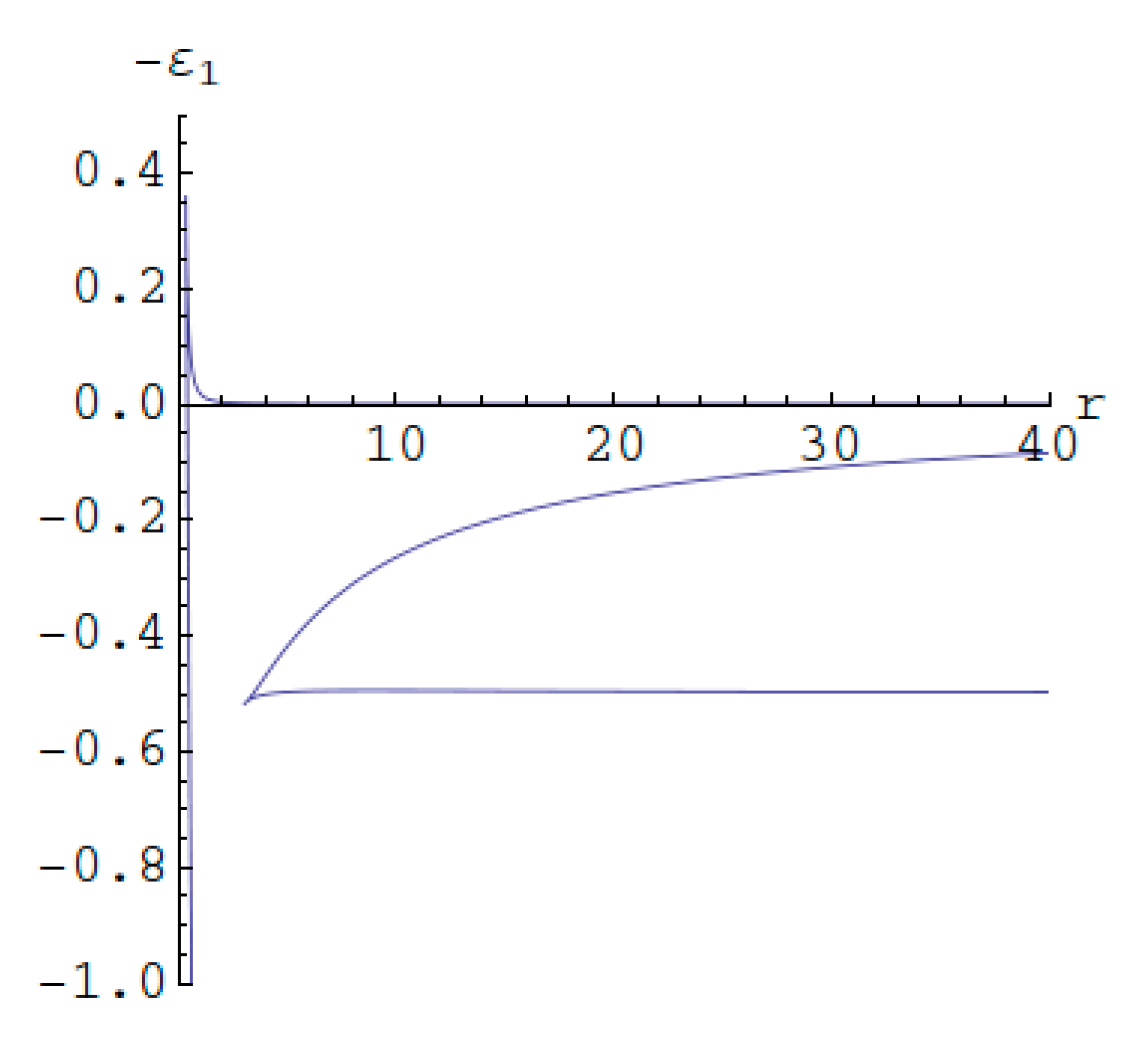


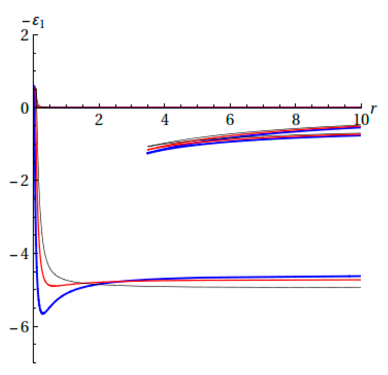
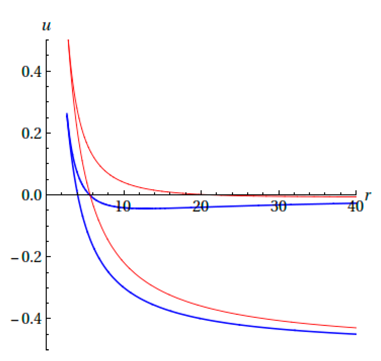