Aerodynamic-Torque Induced Motions of a Spinning Football and Why the Ball’s Longitudinal Axis Rotates with the Linear Velocity Vector

Abstract

This paper presents an explanation of why a spinning football rotates so that the spin axis remains nearly aligned with the velocity vector, and approximately parallel to the tangent to the trajectory. The paper derives the values of the characteristic frequencies associated with the football’s precession and nutation. The paper presents a graphical way of visualizing how the motions associated with these frequencies result in the observed “wobble” of the football. A solution for the linearized dynamics shows that there is a minimum amount of spin required for the motion to be stable and for the football not to tumble. This paper notes the similarity of this problem to that of spun projectiles. The results show that the tendency of a football to align itself with and rotate with the velocity vector is associated with an equilibrium condition with a non-zero aerodynamic torque. The torque is precisely the value required for the football to rotate at the same angular rate as the velocity vector. An implication of this is that a release with the football spin axis and velocity vector aligned (zero aerodynamic torque) is not the condition that results in minimum motion after release. Minimum “wobble” occurs when the ball is released with its symmetry axis slightly to the right or left of the velocity vector, depending on the direction of the spin. There are additional forces and moments acting on the football that affect its trajectory and its stability, but it is not necessary to consider these to explain the tendency of the ball to align with the velocity vector and to ”wobble.” The results of this paper are equally applicable to the spiral pass in American football and the screw kick in rugby.

1. Introduction

This paper will use the generic term “wobble” to describe the general angular motion of the football until we can be precise about what is causing the motion. The term “spin” refers to rotation of the football about its axis of symmetry, and “rotation” refers to angular motion about an axis perpendicular to the spin axis. Because there is no possibility of confusion, angular momentum will be referred to simply as “momentum” The term ball or football will be used interchangeably, and the terms spiral pass or American football, and screw kick or rugby football, will be used when the discussion applies exclusively to only one case. Brancazio [1] suggests that the observable wobble of the American ball in a spiral pass is an example of precession. The author assumes the motion is torque-free; however, there is an aerodynamic torque acting on the football that cannot be neglected if the ball’s velocity-vector-following motion is to be explained. That torque, interacting with the momentum of the spin, is an essential part of the rotational dynamics of the ball. The same author revisits the problem in a later publication [2] assuming the spiral pass is like a “sleeping-top” where the assumption is that the torque is very small; however, the author incorrectly asserts that in the case of a spiral pass, there is no aerodynamic torque and the analysis cannot explain the velocity-following motion. In their introduction, Price et al. [3] observe that the axis of the ball tends to align itself with the tangent to its trajectory, which is equal to the instantaneous velocity of the ball. They reason that since the momentum is predominantly due to spin, the ball’s angular momentum also stays nearly aligned with the velocity. They correctly conclude that because the velocity vector rotates, beginning pointed upward at the release and downward at the catch (or drop), that there must be a torque acting on the ball to cause the angular momentum to change.

Price et al. [3] start with general equations for the angular motion. Rather than derive a solution from those equations, the authors assume a solution based on characteristic frequencies that are not correct for the physical model and do not satisfy the equations of motion. Consequently, their quantitative results are incorrect. This paper derives the correct frequencies from the mathematical model. The explanation in [3] for the velocity-following motion draws on intuition, and the paper does not show that the assumed mathematical model predicts the motion, nor state any necessary conditions that must be satisfied for their explanation to hold. Furthermore, if their intuitive explanation is applied to the case where the nose of the ball is released below the plane of the velocity vector, the explanation predicts that the ball will rotate in a direction opposite from what it actually does. The results in [4] begin by assuming the incorrect characteristic frequencies from [3], and claims to derive a model for “first-order differences between the direction of the velocity, the orientation of the long axis, and the direction of the total angular momentum.” If this is understood to mean linear dynamics near an equilibrium point, then this paper presents the correct solution to that problem.

The dynamics of a spinning football do not represent a type of problem that is new to study. The study of ballistics has led to an understanding of how spin can be used to improve both distance and accuracy of artillery projectiles and rifle bullets. The paper [5] provides a description of the physical mechanism resulting in stable flight, the tendency of a spinning projectile to align with the velocity vector and the cause of the necessary torque, and the resulting tendency of a right-handed spin to cause a drift to the right. Rae [6] identifies these same characteristics associated with the spiral pass in his experimental and analytical results for an American football. The paper [5], published over 100 years ago, describes itself as a “non-technical introduction” to other work that details the state of understanding of the dynamics of spun projectiles. Perhaps the original written reference to discuss the essential physics associated with the trajectory-following behavior is [7], and that author does not claim originality for the ideas in the paper. While there is likely a great deal of additional information accessible on the Internet and stored in government archives, there are two good books [8,9] that present detailed descriptions of how to model the aerodynamic forces and moments on a spun projectile and the resulting dynamics.

The following section derives equations of motion for a spinning football assuming the ball is acted on by only gravity and an aerodynamic torque. The torque acts to turn the nose of the ball away from the direction of flight. In a frame of reference defined by the velocity vector, the equations of motion are approximately linear and can be solved analytically. This solution provides a stability condition in terms of a relationship between the spin momentum and the rate of change of aerodynamic torque with respect to angle relative to the velocity vector. The solution also identifies two characteristic frequencies associated with the motion. The next section provides an interpretation of the analytical solution in terms of a way to visualize the time-varying solution and in terms of quantitative examples. This section focuses on the spiral pass, and presents quantitative results and interpretations of those results that differ from the results in [3]. Whenever this occurs in this paper, the differences are identified and explanations for the differences are provided. A following shorter section considers similar examples for the screw kick. The rugby screw kick differs primarily in the smaller magnitudes of the spin and linear velocities. The conclusions note that this paper only considers one aspect of the problem, and that a more general physical model in line with Rae [6] needs to be considered to fully describe the motion. The results are summarized in a conclusion section which ends by describing the similarity between the dynamics of a football and a terrestrial gyroscope.

2. Modeling the Torque-Induced Dynamics of the Spinning Football

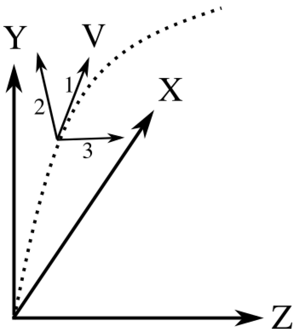
This section describes a mathematical model for the dynamics of a spinning football, derives equations for the linear dynamics, and solves those equations. The section begins with the definition of reference frames. Figure 1 shows a pair of right-handed frames. The larger set of axes is fixed to the field with the X-axis oriented down the field. The model does not include lift, so the ball will remain in the plane defined by X and the axis Y oriented vertically, normal to the playing surface. The Z-axis is oriented to complete a right-handed frame. The dashed line denotes the trajectory of the ball. The smaller frame has its origin at the geometric center of the ball with its 1-axis tangent to the trajectory and its 3-axis perpendicular to the plane containing the trajectory. The small reference frame, with its 1-axis aligned with the velocity, will be the reference frame in which the equations of motion will be solved.

The differential equation describing the motion of the velocity-fixed frame relative to the field-fixed frame is

$$\dot{\overrightarrow{v}}=\left[\begin{array}{c}0\\ -g\\ 0\end{array}\right]\to \left[\begin{array}{c}{v}_1\left(t\right)\\ v_2\left(t\right)\\ v_3\left(t\right)\end{array}\right]=\left[\begin{array}{c}{V}_{0}cos{\Phi }_0\\ V_{0}sin{\Phi }_0-9.81t\\ 0\end{array}\right].$$

(1)

This equation is readily solved given initial velocity $V_0$ and angle ${\Phi }_0$. $\Phi$ denotes the angle between the velocity vector and the horizontal, and g denotes the local acceleration of gravity. The corresponding angular velocity of this frame about the Z or 3-axis is

$${\overrightarrow{\omega }}_v=\widehat{v}\times \dot{\widehat{v}}={\left[0,0,{\omega }_V\right]}^T\to {\omega }_v=-\frac{gcos\Phi }{V}$$

(2)

where V and ${\omega }_v$ denote the magnitudes of the corresponding vectors, and $tan\Phi =v_2/v_1$ is the tangent of the angle between the 1-axis of the velocity-frame and the horizontal plane. Note that $\Phi$ is not related to the orientation of the ball.

Following the example of Price et al. [3], our equations use not the momentum, but the momentum divided by the transverse moment of inertia $I_t$. We will denote this modified momentum $\overrightarrow{h}$ and have for Newton’s Second Law

$$\frac{\dot{\overrightarrow{H}}}{I_t}=\dot{\overrightarrow{h}}=\frac{\tau }{I_t}$$

(3)

where $\tau$ is an aerodynamic torque defined shortly. The symbol $\widehat{s}={[s_1,s_2,s_3]}^T$ denotes a unit-vector oriented along the spin-axis of the football. The differential equation for $\widehat{s}$ is

$$\dot{\widehat{s}}=\overrightarrow{h}\times \widehat{s}.$$

(4)

Since $\widehat{s}$ is a unit vector, we can compute $s_1$ from the other two values, so the first equation in Equation (4) is not strictly necessary. These are the equations of motion that have been used in the previously cited references on football dynamics. They are defined in the field-fixed frame of reference in Figure 1. The term rotation always refers to the motion of the unit vector described by Equation (4), spin always refers to the angular motion of the ball about $\widehat{s}$. The reference frame moving with the ball in Figure 1 is defined to follow the dashed line in the figure. The 1-axis of this frame remains tangent to the dashed line. Writing Equations (3) and (4) in this velocity-fixed frame rotating at angular velocity ${\overrightarrow{\omega }}_V$ yields [10]

$$\dot{\overrightarrow{h}}+{\overrightarrow{\omega }}_V\times \overrightarrow{h}=\frac{\tau }{I_t}$$

(5)

and

$$\dot{\widehat{s}}+{\overrightarrow{\omega }}_V\times \widehat{s}=\overrightarrow{h}\times \widehat{s}=\left[\begin{array}{c}{h}_2{s}_3-h_3{s}_2\\ h_3{s}_1-h_1{s}_3\\ h_1{s}_2-h_2{s}_1\end{array}\right].$$

(6)

The advantage of writing the equations of motion in this frame is that small angle approximations apply, and the equations for the rotation of the ball can be solved analytically. In these equations, $\widehat{s}$ and $\overrightarrow{h}$ are defined in the 1–2–3 frame, and if the initial conditions are not too large, these vectors will remain close to the velocity vector.

Using the notation in McCoy [8], the aerodynamic torque associated with the overturning moment is

$$\begin{array}{ccc}\hfill \tau & =& \frac{1}{2}\rho SD\parallel \overrightarrow{v}\parallel C_{M_{\alpha }}\overrightarrow{v}\times \widehat{s}=\frac{1}{2}\rho SD{V}^2{C}_{M_{\alpha }}\widehat{v}\times \widehat{s}=I_t{M}_{\alpha }{\left[0,-s_3,s_2\right]}^T\hfill \\ \hfill M_{\alpha }& =& \frac{\rho SD{V}^2{C}_{M_{\alpha }}}{2I_t}\hfill \end{array}$$

(7)

where D is the maximum diameter of the ball, S is the area $\frac{\pi }{4}{D}^2$, and $\widehat{v}=[1,0,0]$ is the unit vector corresponding to $\overrightarrow{v}$. Note that Equation (7) implies that the torque is perpendicular to both the velocity and the spin-axis. The symbol $C_{M_{\alpha }}$ denotes the slope at the origin of the aerodynamic coefficient associated with the overturning moment. This implies that a linear approximation is made. In the general case, the torque coefficient would be modeled using a Taylor series (analytical model for $C_M$) [11], a power series (polynomial fit to data), or a table lookup that are functions of the angle between $\widehat{v}$ and $\widehat{s}$, $\delta$, where $sin\delta =\widehat{v}\times \widehat{s}$.

Combining these last three equations, eliminating the equation for ${\dot{s}}_1$, and assuming ${\omega }_V{h}_2\ll {\omega }_V{h}_1$, which implies $h_1$ is constant, yields in the rotating frame

$$\left(\begin{array}{c}{\dot{s}}_2\\ {\dot{s}}_3\\ {\dot{h}}_2\\ {\dot{h}}_3\end{array}\right)=\left[\begin{array}{cccc}0& -h_1& 0& s_1\\ h_1& 0& -s_1& 0\\ 0& -M_{\alpha }& 0& 0\\ M_{\alpha }& 0& 0& 0\end{array}\right]\left(\begin{array}{c}{s}_2\\ s_3\\ h_2\\ h_3\end{array}\right)+\left(\begin{array}{c}-{\omega }_V{s}_1\\ 0\\ -{\omega }_V{h}_1\\ 0\end{array}\right).$$

(8)

If the angle between the spin or longitudinal axis of the ball and the velocity vector is small, then we may also assume that $s_1\approx 1$. Differentiating the first two equations in Equation (8) with respect to time, and using the second two to substitute for $\dot{h_2}$ and $\dot{h_3}$ in those equations yields a pair of coupled second-order equations.

$$\begin{array}{ccc}\hfill {\ddot{s}}_2+h_1{\dot{s}}_3-M_{\alpha }{s}_2& =& 0\hfill \\ \hfill {\ddot{s}}_3-h_1{\dot{s}}_2-M_{\alpha }{s}_3& =& -{\omega }_V{h}_1\hfill \end{array}.$$

(9)

Multiplying the second equation by $i=\sqrt{-1}$, substituting $x=s_2+i{s}_3$, and $-ix=-i{s}_2+s_3$ yields the single equation

$$\ddot{x}-i{h}_1\dot{x}-M_{\alpha }x=-i{\omega }_V{h}_1.$$

(10)

The solution of this linear constant coefficient equation consists of a particular and a complementary part. A particular solution can be obtained by simple inspection as

$$-M_{\alpha }{x}^p=-M_{\alpha }(s_2^p+i{s}_3^p)=-i{\omega }_V{h}_1\to -s_3^p{M}_{\alpha }=-{\omega }_V{h}_1\to s_3^p=\frac{gcos\Phi h_1}{M_{\alpha }V}.$$

(11)

The real part of the particular solution $s_2^p=0$. For small angles, $s_3$ is the angle between the vertical plane of the trajectory and the axis of the ball, so $-s_3^p{I}_t{M}_{\alpha }$ is the torque about the 2-axis in the velocity-frame. The term $-{\omega }_V{I}_t{h}_1$ is the rate of change of the spin angular momentum of the football as it follows the trajectory. This demonstrates that the physical model Equations (5) and (6) predicts that the paradoxical behavior described in Price et al. [3] occurs. The condition where the ball is rotated away from the velocity vector by $s_3^p$ and rotating at an angular velocity ${\omega }_v$ corresponds to the equilibrium state of the physical model expressed as any of Equations (8)–(10). The equilibrium condition does not correspond to a condition where the aerodynamic torque is zero.

Using the quadratic formula to determine the roots of the characteristic equation associated with the left-hand side of Equation (10) yields the complementary solution. Adding the complementary solution to the particular solution Equation (11) yields

$$\begin{array}{ccc}\hfill x\left(t\right)& =& s_2+i{s}_3+i{s}_3^p\hfill \\ \hfill & =& C_1{exp}^{0.5\left(i{h}_1+\sqrt{-h_1^2+4M_{\alpha }}\right)t}+C_2{exp}^{0.5\left(i{h}_1-\sqrt{-h_1^2+4M_{\alpha }}\right)t}+i\frac{gcos\Phi h_1}{M_{\alpha }V}.\hfill \end{array}$$

(12)

where the complex constants $C_1$ and $C_2$ are chosen to satisfy the initial conditions. The complementary solution of the above equation consists of two complex exponential parts with time constants equal to $0.5\left(i{h}_1\pm \sqrt{-h_1^2+4M_{\alpha }}\right)$. The roots will be purely complex if $h_1^2>4M_{\alpha }$, and any solution of these differential equations will have finite values; otherwise, one pair of roots will have a positive real part and the solution will be unstable. This inequality is the necessary and sufficient condition to ensure that the solution of Equations (5) and (6) is stable. Assuming this “gyroscopic stability” criterion is satisfied, the coefficients multiplying time are purely complex numbers and the complementary solution is the sum of a pair of harmonic oscillators at two different frequencies. Letting the symbols ${\omega }_f$ and ${\omega }_s$ denote the values of the larger (fast) and smaller (slow) frequencies corresponding to first and second exponents in Equation (12), the equations for the values of the complex constants are

$$C_1\left({\omega }_f-{\omega }_s\right)={\dot{s}}_3-i{\dot{s}}_2-{\omega }_s{s}_2-i{\omega }_s\left(s_3-s_3^p\right)$$

(13)

and

$$C_2\left({\omega }_f-{\omega }_s\right)=-{\dot{s}}_3+i{\dot{s}}_2+{\omega }_f{s}_2+i{\omega }_f\left(s_3-s_3^p\right)$$

(14)

The solution Equation (12) can be applied at any point along the trajectory of the ball to understand the local (in time) behavior of the pass. The wobble is composed of the sum of a pair of complex oscillators with the frequency dependent on the velocity and the physical characteristics of the ball. These oscillations are centered in the state-space about a point that is slightly offset from the origin in a direction perpendicular to the direction of flight. The location of this point depends on the velocity vector in such a way that the average torque (as the ball wobbles about this point), is exactly the amount required for the average rotation rate of the ball to match the rotation rate of the velocity vector. The state $(0,s_3^p)$ is an equilibrium point. Note that a ball thrown with this initial condition and $\dot{\widehat{s}}=0$ corresponds to $C_1=C_2=0$ and the ball will exhibit no wobble. The next section will discuss a way to visualize these solutions.

At this point it is possible to discuss some of the shortcomings of the explanation for the velocity-tracking behavior of the ball in Price et al. [3]. That explanation requires an initial angle of attack in the vertical plane. The torque associated with this angle of attack causes a torque that results in the nose of the ball rotating to the left or right of the plane of the trajectory depending on the spin. It is argued that this is what causes the sideslip angle that results in the torque Equation (11). It is also argued that this necessarily results in precession and nutation. The solution above shows that none of this is necessary. The necessary sideslip will develop even if the angle of attack is zero and there is no wobble. If the initial condition of the ball is such that the nose of the ball is below the velocity vector or the initial angular velocity is large enough for the angle of attack to become negative, the argument provided in [3] will cause the sideslip to have the opposite sign, the torque will have the opposite sign, and the explanation predicts the angular rotation of the ball will be in the incorrect direction.

3. Explaining the Torque-Induced Motion of the Spiral Pass

This section examines the motion of a spiral pass by introducing into the mathematical model the physical characteristics of an American football. The section introduces a method for the reader to visualize how the two oscillators in the solution combine to produce the observed motion. The wind-tunnel measurements [12] seem to be the only available data for the American football’s overturning moment and suggest a value of $C_{M_{\alpha }}=0.33{\mathrm{rad}}^{-1}$. The units are added to the aerodynamic coefficient to indicate it is the slope of the non-dimensional moment-coefficient curve. Rae and Streit [12] suggests using $C_M=0.165sin\left(2\delta \right)$ for angles up to $50\mathrm{deg}$. The inertia properties of the football [6] are $I_t=0.00321\mathrm{kg}{\mathrm{m}}^2$ and $I_s=0.00194\mathrm{kg}{\mathrm{m}}^2$. These values are reported as measured, but the citation is a personal communication. The nominal release velocity considered is $27.4\mathrm{mps}$ which is slightly over $60\mathrm{mph}$, an angle of $30\mathrm{deg}$ above the horizontal, and a spin rate of $600\mathrm{rpm}$. Using this information yields $M_{\alpha }=191$ and $h_1=38$, which in combination with Equation (12) yields a differential equation for the rotational motion of a football

$$x\left(t\right)=C_1{\mathrm{e}}^{32.01it}+C_2{\mathrm{e}}^{5.958it}+0.0617i\approx C_1{\mathrm{e}}^{\left(2\pi \right)5it}+C_2{\mathrm{e}}^{\left(2\pi \right)it}+0.06i.$$

(15)

In the above equation on the right, the two natural frequencies of the football are expressed in Hertz. The fast mode, ${\omega }_f$, has a frequency of about $5\mathrm{Hertz}$ and the slow mode, ${\omega }_f$, has a frequency of about $1\mathrm{Hertz}$. For a long pass lasting about $3\mathrm{s}$, there will be 15 orbits of the fast mode and 3 of the slow-mode. The fast-mode frequency of $32\mathrm{rad}{\mathrm{s}}^{-1}$ differs from the value ${\omega }_{wob}=38$ given in Table 1 of Price et al. by about $20\%$; however, the slow-mode frequency of the actual solution is $2.4$ times the value of ${\omega }_{gyr}=2.52$. The formula the authors use to compute ${\omega }_{gyr}$ can be found in the paper by Soodak [13]. Soodak’s Equations (1) and (1a) are identical to Equations (3) and (4), respectively, except with the added assumption that the torque $\tau$ is constant. Price et al. do not apply the formula for ${\omega }_{gyr}$ in Soodak [13] correctly. According to their Equation (3), the symbol ${\tau }^{\ast }$ must be multiplied by the sine of the angle between the spin axis and the velocity vector to obtain the torque. There are two angles that could be used. One of those is zero, corresponding to alignment with the velocity vector, in which case ${\omega }_{gyr}=0$. This corresponds to torque-free motion, and it is evident their paradox cannot be resolved under this assumption. The other possibility is to use the angle ${sin}^{-1}{s}_3^p\approx s_3^p$ in which case ${\omega }_{gyr}=\left|{\omega }_V\right|$, namely, the angular rotation of the velocity vector. This choice is consistent with the assumptions associated with Equation (1a) in Soodak [13]. that requires that the torque be constant, which is contradictory to how it is used in [3]. While the error in the frequency ${\omega }_{wob}$ could be argued to not be significant, this error effectively invalidates the quantitative results in [3,4].

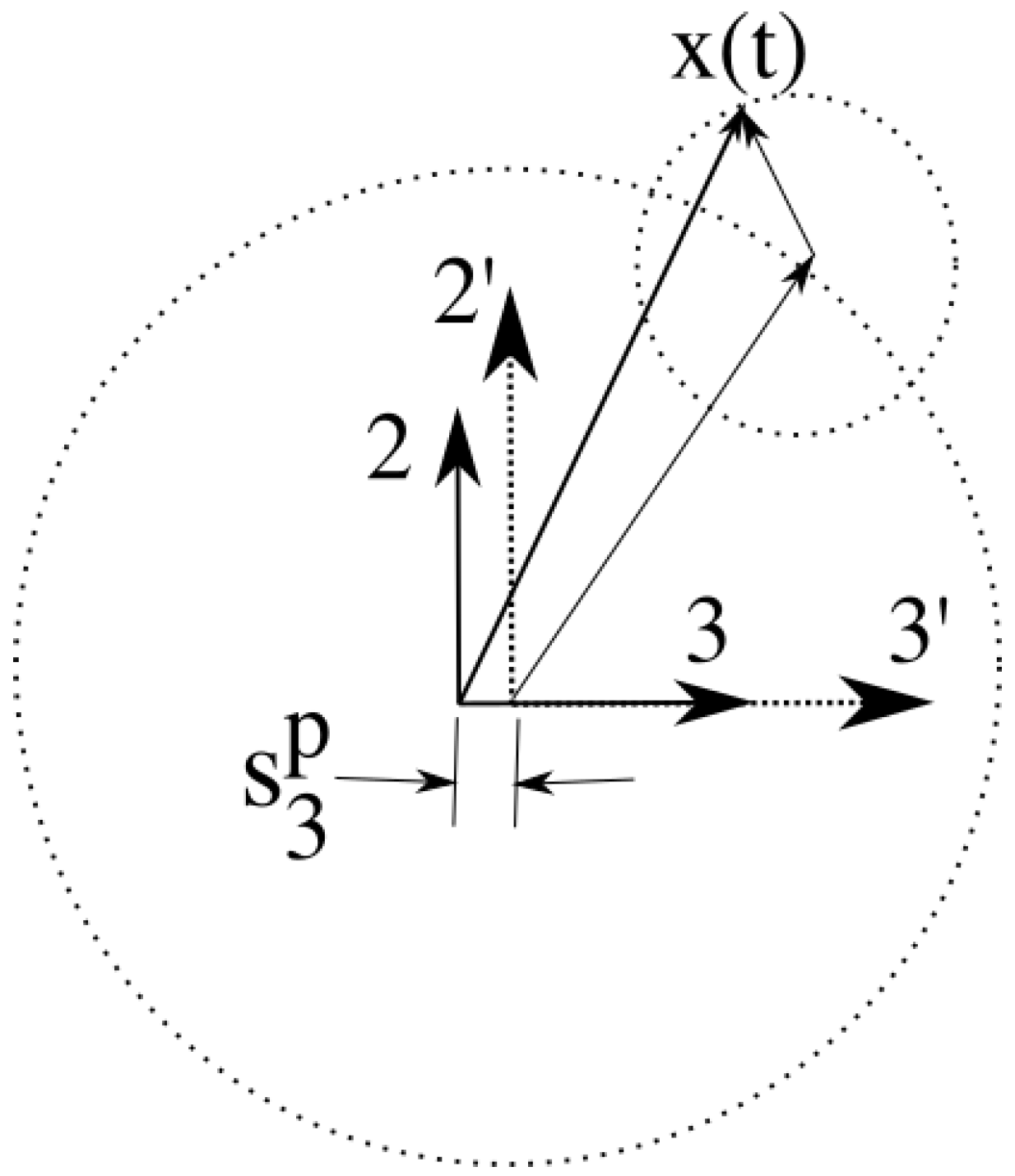
Before discussing additional solutions of Equation (15), it is useful to introduce a way to visualize the motion of the football implied by the equation. Figure 2 shows two axes (solid lines) of the velocity-fixed frame of Figure 1. The view in this figure is along the 1-axis of the velocity vector. The 2-axis corresponds to the real component of the solution x and the 3-axis the complex part. Recalling that $\widehat{s}$ is a unit vector along the ball’s spin-axis, plotting the components $s_2$ and $s_3$ correspond to plotting the projection of $\widehat{s}$ on this coordinate plane. Solutions of Equation (15) will typically have the characteristic that the slow-mode has a larger amplitude than the fast mode when the magnitude of $\dot{x}\left(0\right)$ is equal to or smaller than $x\left(0\right)$ because of the differences in magnitudes of the constants in the exponents. Stated differently, if $|C_1|\approx |C_2|$, then the initial magnitude of $\dot{x}$ will be about five times larger than the magnitude of x, which likely corresponds to a badly thrown pass. Note that if $\dot{x}={\dot{s}}_2={\dot{s}}_3=0$, it follows from Equations $C_1$ and $C_2$ that $|C_1|$ cannot be larger than $|C_2|$. Assume for a moment that $C_1=0$ and only the slow-mode is evident in the solution. The long arrow in Figure 2 represents the value of the complex solution for this case. As time moves forward, this arrow traces out the large dashed circle at the slow-mode frequency, clockwise for a right-handed pass. The figure indicates that the center of this circle is not the origin of the frame, but is shifted slightly to the right due to the particular solution $s_3^p$. The center of rotation associated with this motion is the primed reference frame with dashed axes. In the illustrated case, the passer is right-handed because this shift is positive. When $C_1$ is not zero, its contribution to the complex solution is also a circular orbit except at the fast frequency. This can be visualized as the shorter vector added to the slow-mode vector. The fast mode traces out the small dashed circle at the fast frequency, clockwise for a right-handed throw. The origin of this point of rotation for the fast mode moves along the circle defined by the vector associated with the slow-mode at the slow frequency. The combined effect is well-characterized by the word wobble.

Precession can be defined as an Euler angle associated with a vector rotated about an axis. In the case here that would be the angle of x measured about the $1^{\prime }$-axis in Figure 2 and referenced to either the 2 or 3 axes. Nutation can be defined as the Euler angle between the $1^{\prime }$-axis and the point $\widehat{s}\left(t\right)$; the sine of this angle is equal to the magnitude of the complementary part of the solution of $x\left(t\right)$. Note that as long as $s_3^p$ is small, the distinction between angles measured in the two frames is not significant. Based on the discussion of the previous paragraph, the precession mode will be associated with the frequency associated with the larger of $|C_1|$ or $|C_2|$. Price et al. [3] repeatedly assert that precession occurs at the fast frequency. This seems to be an assumption on their part, as it is clear that this depends on the initial conditions. Experience with solutions of Equation (12) suggests that for the spiral pass, the precession frequency is always the slow mode frequency for a well-thrown football and that large values of ${\dot{s}}_2\left(0\right)$ and ${\dot{s}}_3\left(0\right)$ (relative to $s_2$ and $s_3$) need to be assumed to change this. This statement might be formalized given a definition of a well thrown pass in terms of the absolute magnitude of $x\left(0\right)$ and its magnitude relative to $\dot{x}\left(0\right)$. If the torque on the ball were suddenly removed, the precessional motion associated with the longer vector in Figure 2 would abruptly cease and that vector would stop rotating. The shorter vector would continue to rotate about the stationary tip of the longer vector except at the torque-free frequency $h_1{I}_t/I_s$.

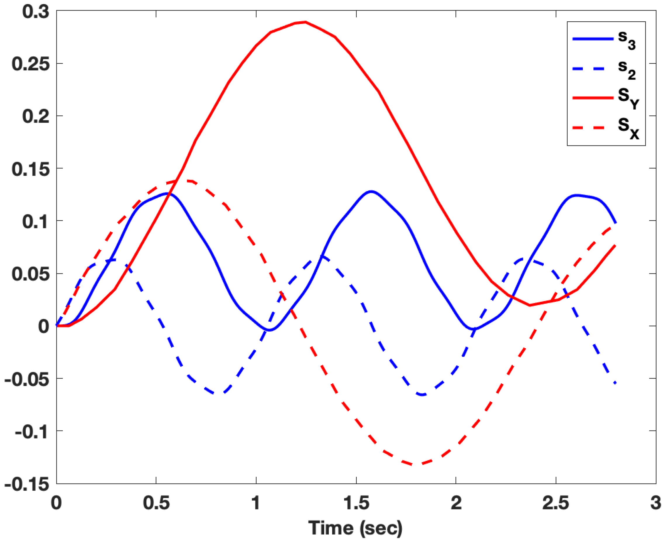
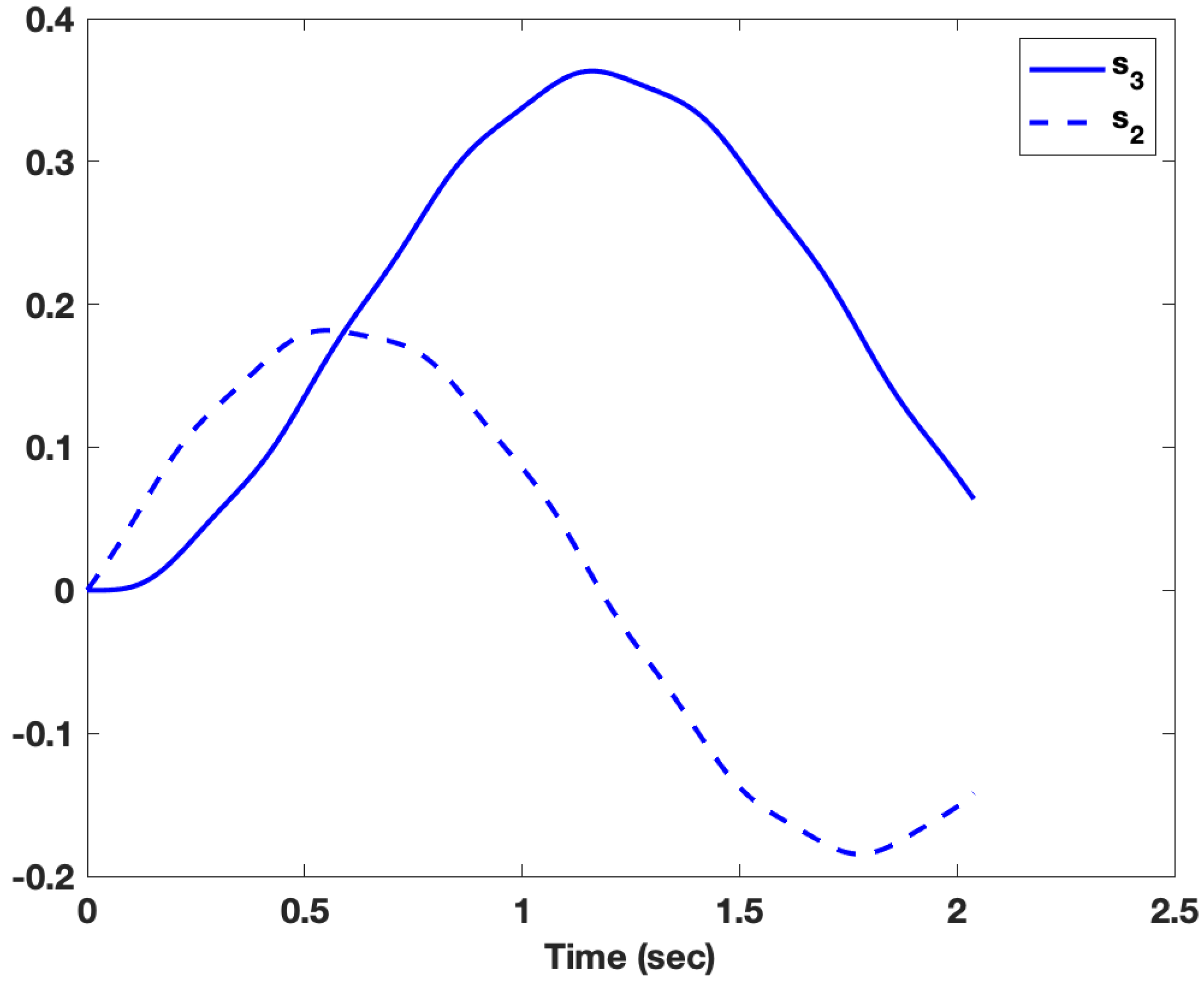
The image in Figure 3 shows a solution of Equation (15) under the assumption that the ball is released with its symmetry axis and the velocity vector initially aligned, and the symmetry axis is not rotating relative to the field. This corresponds to $C_1=0.002214$ and $C_2=-0.06339$. Since $C_1$ is much smaller than $C_2$, the solution will be dominated by the slow mode. These initial conditions have been associated with a notion of a perfect pass, ref. [3] and correspond to the results in Figure 3 of that reference. The red lines in the figure are data digitally sampled from that figure. The same $2.8\mathrm{s}$ duration of the simulation was also used in Equation (15) and are plotted in blue. It is evident that there is a significant difference in the frequency of the motion computed in Price et al. and that predicted by the analytical solution of the equations. This is evident in all of the quantitative results of Price et al. The predicted lateral offset associated with the mean value of $S_Y$ is also much larger that the value computed analytically. This suggests that the torque coefficient used may have been too small, but that is not the only possibility.

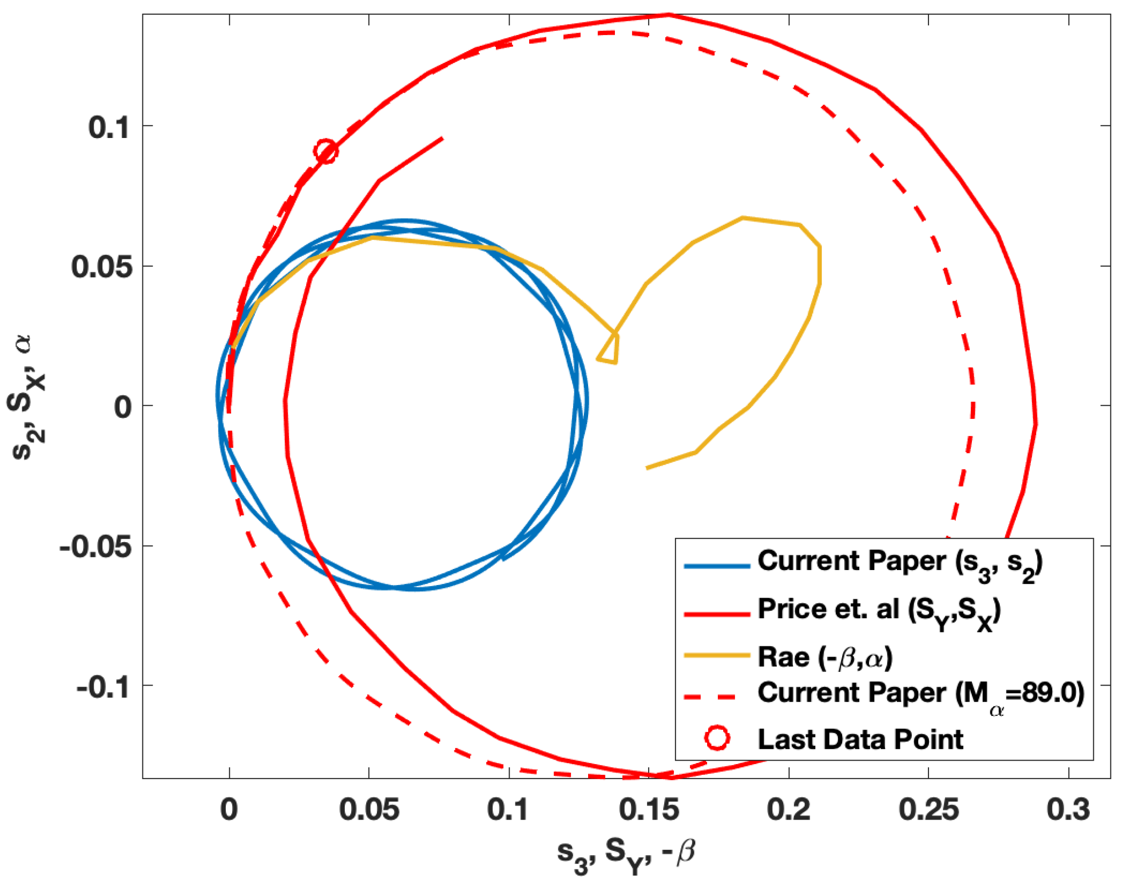
A different comparison with the analytical solution to this result in Price et al. is given in Figure 4. The solid blue and red circles are the same data as in Figure 3, and correspond to the analytical solution here and the data from Price et al., respectively. This figure also includes data sampled from Figure 9 of Rae [6]. We do not agree with the claim by Price et al. that their results compare favorably with Rae. The apparent agreement with the solution computed here and Rae suggested by Figure 4 is possibly misleading. A comparison of time-series is required to determine if there is agreement. This difference is expected though. The problem solved by Rae is substantially different than the one solved here. The dashed line in the figure was computed using the analytical solution but with a value of $M_{\alpha }=89$; namely, half the correct value. The small red circle indicates where that solution ends at $2.8\mathrm{s}$, close to where the solution by Price et al. ends. This change yields a result more similar to Price et al., but is not sufficient to explain how their results were actually computed. The value 89 is based on using half the value of ${\tau }^{\ast }=0.308$ from Table 1 in Price et al. While the difference is not significant, the value used by Rae [6] is $0.33$. Since the physical model assumed in this paper and [3] are the same, the results of the last two figures indicate that the numerical method used by Price et al. contains an error.

In the paper by Price et al., the authors do not make the proper distinction between the terms pitch angle and yaw angle, and the terms angle of attack ($\alpha$) and sideslip angle ($\beta$) [14]. They incorrectly state that Rae uses the term slideslip [sic], suggesting that no distinction is in fact being made. Price et al. use the terms pitch and yaw in place of the correct aerodynamic terms; for example, after Figure 4 in their paper. Pitch angle and yaw angle refer to the orientation of the axis of the ball relative to a reference frame fixed to the field. These are Euler angles associated with their vector $\widehat{s}$ relative to the field-fixed frame. Angle of attack and sideslip are Euler angles associated with the orientation of the ball relative to the velocity vector and are associated with their vector components $S_X$ and $S_Y$. These four angles are all independent variables of the motion in the three dimensional case. The sideslip and yaw angle are equal in this paper and the paper by Price et al. only because the motion is constrained to be in a vertical plane; in general, they will be different. In the paper by Rae [6] they are different, and the distinction is evident in the results. In Rae’s paper, Figures 5, 7 and 9 plot the angle of attack vs. sideslip, and Figures 6, 8, and 10 plot pitch angle ($\theta$) vs. yaw angle ($\psi$). Each pair of plots is very different. If the angle between the axis of the ball and the velocity vector is small, then $\alpha \approx S_X=s_2$ and $-\beta \approx S_Y=s_3$. It is essential when instructing students on material like this to make the proper distinction between pitch/yaw and angle of attack/sideslip. In many cases they are identical (e.g., in a wind tunnel), and failure to recognize the difference can lead to confusion. It is also essential to clear communication.

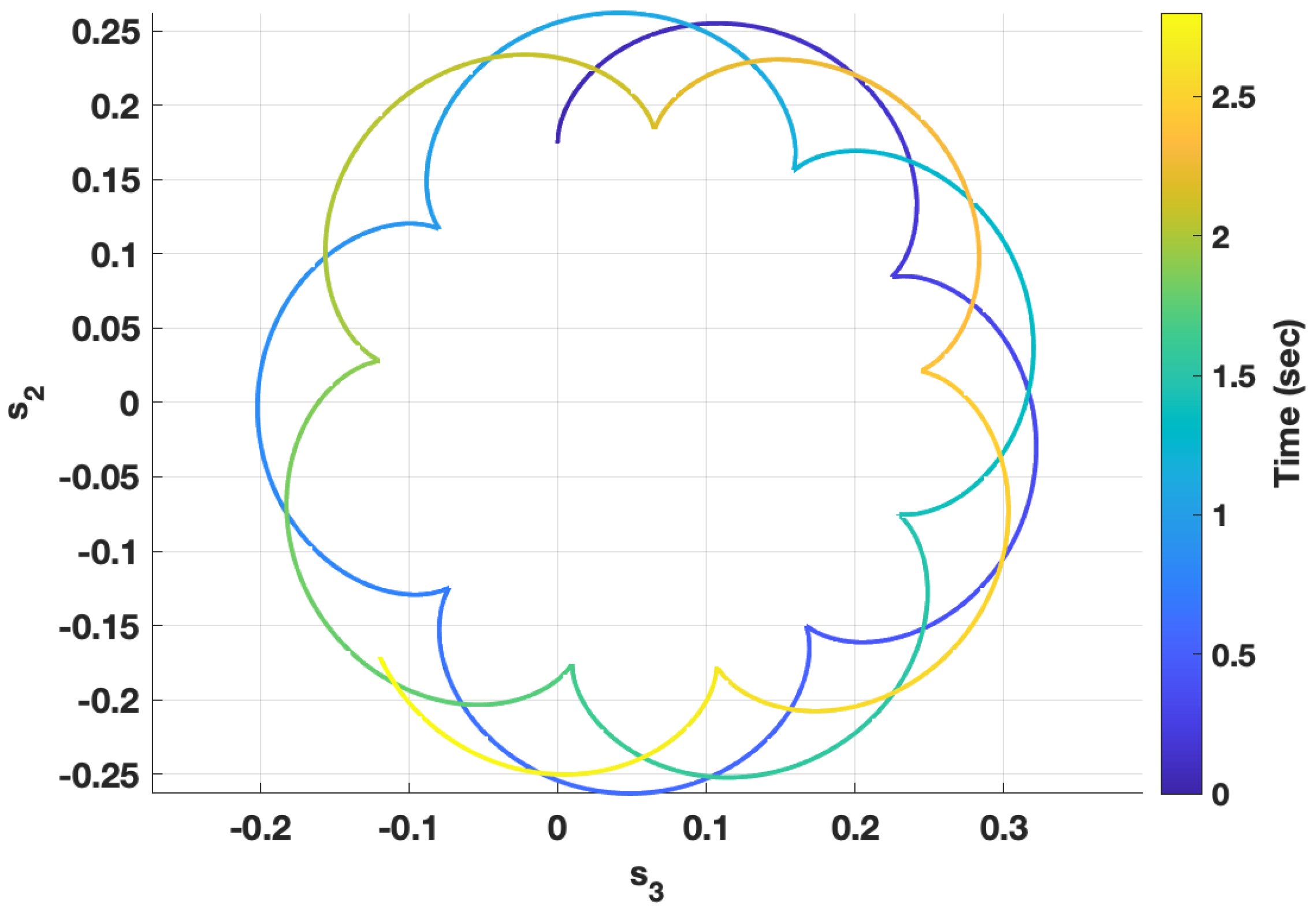
Figure 5 shows the solution of Equation (15) assuming the nose of the football is released $10\mathrm{deg}$ above the velocity vector and not rotating relative to the field. This corresponds to $C_1=-0.03990+0.002214i$ and $C_2=0.2144-0.06394i$. These results correspond to the less than perfect pass in Figure 7 [3] and Figure 5 [6]. This example provides an opportunity to demonstrate how to apply the interpretation of the motion in terms of the discussion associated with Figure 2. The long arrow associated with the slow-mode rotates with its tip midway between an inner-circle defined by the cusps, and a circle that just contains the entire motion. The tip of this arrow transcribes that circle from its center at $s_3=0.063$. The tip of the short arrow associated with the fast mode follows the line shown in the figure. The effect of this motion includes a component toward and away from the center and this is nutation. In this case, the angular velocity associated with nutation is nearly constant, but the angular velocity associated with precession varies substantially. It is larger when the tip of the fast mode frequency is moving in the same direction as the slow-mode, and slower otherwise.

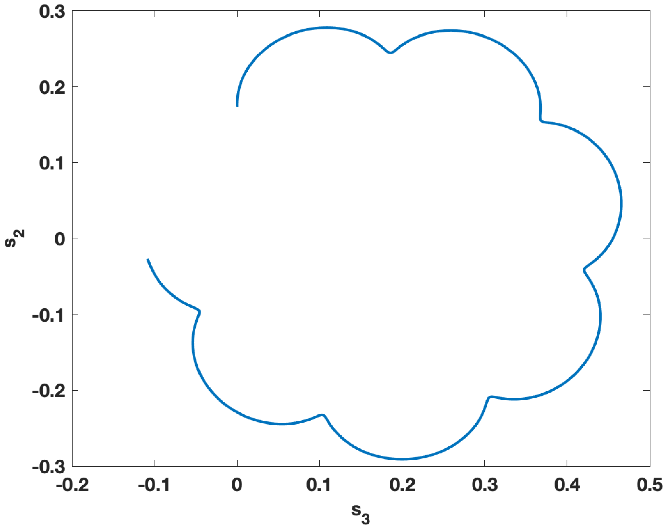
The result in Figure 6 corresponds to the ball being released with the ball-axis aligned with the velocity vector and not rotating vertically. The initial value of ${\dot{s}}_3$ is chosen to correspond to the ball’s nose rotating to the right at a rate of $30\mathrm{deg}/\mathrm{s}$. As with the previous example, the ball’s nutation angle has an approximately periodic character as it moves toward and away from the axis of rotation. The precession angle occasionally moves back upon itself. For this to happen, the angular velocity associated with the precession Euler angle must occasionally be negative for short periods of time.

4. Examples Considering the Rugby Screw Kick

Thy physical model presented here is equally applicable to the motion of the screw kick, if the physical parameters for a rugby ball are used in the equations. The rugby ball is similar in size and shape to the American football. The paper [15] reports a value $C_{M_{\alpha }}=0.147$ for the lift coefficient slope. The aerodynamic data in [15] is normalized by the volume of the ball. The value of $0.147$ was obtained by multiplying the reported value by the ratio of maximum cross-section to volume so that the value is comparable to the value reported by Rae and Streit [12]. The resulting value is less than half that reported for the American football. This difference seems large given the similarity in shapes of the ball. There does not seem to be any obvious systematic error in either paper other than to observe that these measurements are difficult to make in a wind tunnel. The difficulty arises from the need to attach the model to a sting, and there is no good way to remove the effect of the sting on the measurements.

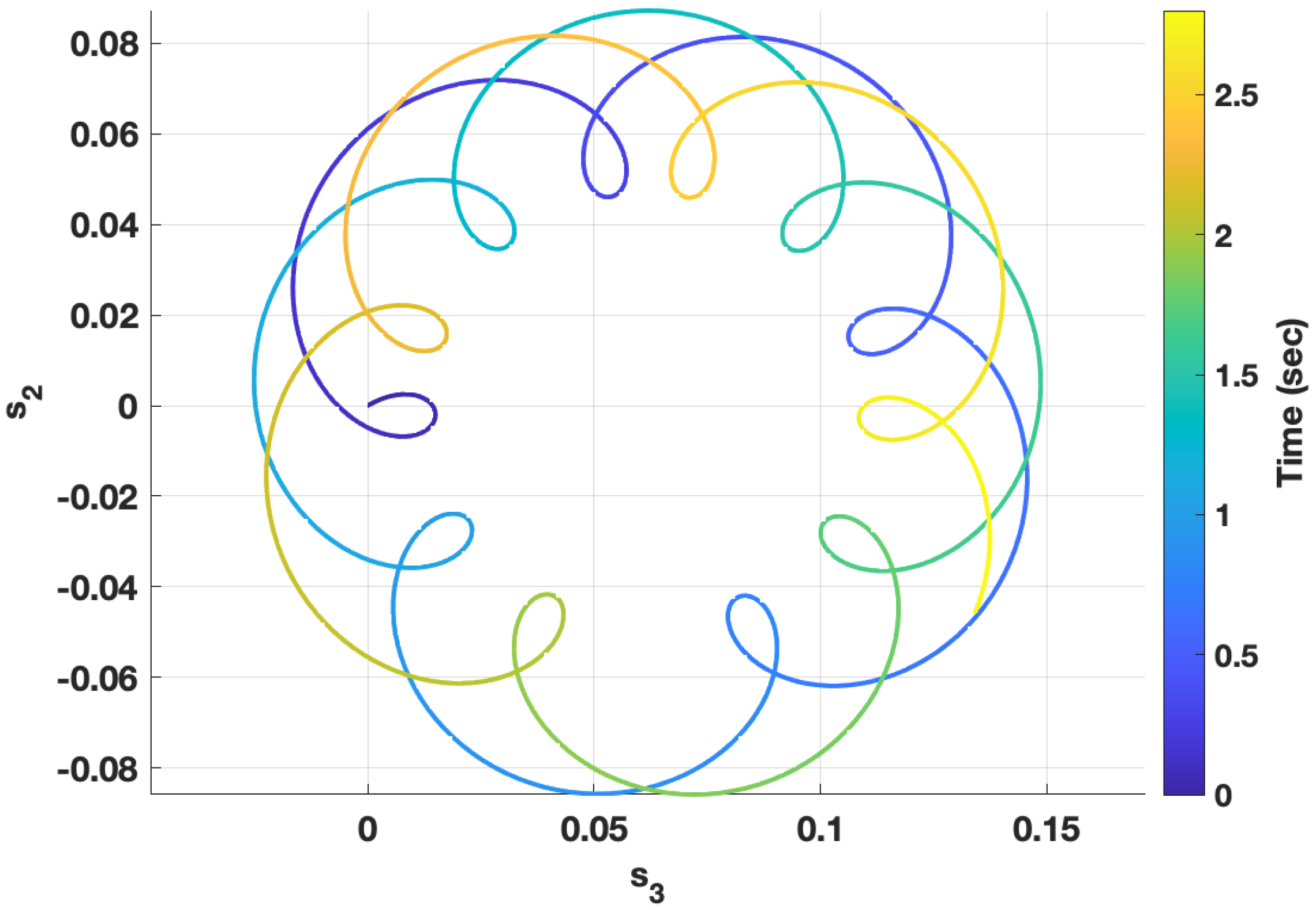
The paper [15] uses a formula from [2] for a thin-walled ellipsoid to calculate values of $I_s=0.0026$ kg-m${}^2$ and $I_t=0.0033$ kg-m${}^2$ for the moments of inertia of the rugby football. The paper [6] compares measured inertia values with the results using the formula, and the agreement is good; especially, for the ratio of the two moments of inertia. The paper [16] suggests ranges for the velocity of the screw kick of 15–25 $\mathrm{mps}$ and for the spin rate of 60–600 $\mathrm{rpm}$. For the analysis presented here, a velocity of $20\mathrm{mps}$ and spin rate of $300\mathrm{rpm}$ are used. Under these conditions, the time-of-flight is just over $2\mathrm{s}$. Note that the the stability criterion for the ball in the screw kick fails to be satisfied for a spin rate of about $131\mathrm{rpm}$. For the selected velocity and spin rate, the frequencies associated with the complimentary solution are ${\omega }_f=22.1\mathrm{rad}{\mathrm{s}}^{-1}\left(3.52\mathrm{Hz}\right)$ and ${\omega }_s=2.65\mathrm{rad}{\mathrm{s}}^{-1}\left(0.422\mathrm{Hz}\right)$. Assuming the screw kick leaves the foot with the symmetry axis and the velocity vector aligned, the solution of the linearized dynamics is plotted in Figure 7. This initial condition corresponds to the conditions of Figure 3, except that the spin rate and velocity are slower for the rugby ball. The results show that for the $2\mathrm{s}$ time-of-flight the total precession is slightly less than one rotation. Like the spiral pass of the American football, this initial condition results in little nutation. This figure also shows that the average value of $s_3$ is around $10\mathrm{deg}$. This is the angle required to yield an average aerodynamic torque large enough to cause the ball to rotate with the velocity vector. The result in Figure 8 is for an initial condition with the symmetry axis of the ball initially $10\mathrm{deg}$ above the velocity vector. This release is the same as that in Figure 5, except for the spin rate and velocity. Note that the maximum amplitude of $s_3$ is over $20\mathrm{deg}$, which is around the limit where we would expect the small angle assumption made to begin to be inaccurate. Equation (11) indicates that the magnitude of $s_3^p$ is proportional to the inverse of the cube of the velocity, so modest decreases in the velocity will result in proportionately larger increases in the average sideslip angle. This suggests that studies of rugby screw kicks should be performed with non-linear models.

5. Conclusions

This paper addressed the question of why the symmetry-axis of a spinning football tends to align itself with its velocity vector. Previous papers correctly hypothesized that this was caused by a torque acting on the football, but did not provide mathematical evidence derived from a hypothesized physical model that this should be the case. This paper showed that a simple model including only gravity and an aerodynamic torque predicted the phenomena. This paper showed that the equilibrium state of the physical model is associated with a torque that exactly causes the required rotation and that the ball’s precession and nutation is centered about this state. This paper also presented a way of interpreting the interaction of the two harmonic modes of the football’s motion. The paper also showed that the frequencies ${\omega }_{wob}$ and ${\omega }_{gyr}$ [3,4], assumed to be characteristic of the motion of a spiral pass, are not correct for an American football. Finally, several quantitative examples were discussed comparing our solutions with prior results, and illustrating the character of the motion of the football when subject only to gravity and an aerodynamic torque. Results were presented for both a spiral pass and a screw kick. The results suggest that at the lower velocities of the rugby ball, a non-linear analysis may be required.

It is important to realize that the equations described here and in the literature associated with the question of the paradox are a simplification of the motion. During the pass considered in the examples, the change in velocity from release to the apex of the trajectory results in a reduction of the moment coefficient by $25\%$. There are also other forces and moments. The results of Rae [6] additionally consider lift, drag, and the Magnus force. Rae and Streit [12] conclude that the Magnus moment is negligible relative to the force. This may be correct, but it is counter to experience with projectiles [8]. The results of this paper should be interpreted as approximating the behavior over short periods of time, and not the entire trajectory. No prior works seem to consider the effect of aerodynamic damping on the motion of the football during the spiral pass or screw kick. One of these moments acts to reduce the spin-rate, and the other the precession and nutation rates. Because of the higher angular velocities associated with the fast mode, this effect will tend to have a stronger effect on that motion. It may be useful to revisit the modeling of the general motion of the pass to validate the results of Rae [6] and to consider the impact of the damping moments on the motion. It would also be useful to derive the sufficient stability condition in the general case.

Price et al. [3] in their paper explicitly reject that there exists an analogy between the motion of a gyroscope and a spiral pass. Consider a frictionless gyroscope placed on a frictionless table in a vacuum. The equations of motion of the football and the gyroscope are nearly identical, the only difference is the physical origin of the torque; gravity in the case of a gyroscope and air flow in the case of a football. If the table is sitting on the surface of the Earth, the surface of the table will rotate. After an extended period of time, the axis of the gyroscope will still be nearly perpendicular to the table. For this to happen, there must be a torque acting on the gyroscope. This torque arises because the axis of the gyroscope is on average tilted slightly to the south. A mathematical analysis of this problem will show that essentially the same equations describe the terrestrial gyroscope as the spiral pass, with the rotation of the gravity vector replacing the rotating velocity vector. A stability criterion similar to the one derived here also arises in the solution of the equations for the terrestrial gyroscope. In closing, we note that the papers [3,4] contain quantitative errors, significant errors in interpretation, and incorrect use of terminology. The resolution given for the paradox does not cover all possible situations, including the one where the nose of the ball is released below the velocity vector. The papers are perhaps detrimental to understanding the problem considered in this paper.

References

- Bancazio, P. Why does a football keep its axis pointing along its trajectory? Phys. Teach. 1985, 23, 571–573. [Google Scholar]
- Brancazio, P. Rigid-body dynamics of a football. Am. J. Phys. 1987, 55, 415–420. [Google Scholar] [CrossRef]
- Price, R.; Moss, W.; Gay, T. The paradox of the tight spiral pass in American football: A simple resolution. Am. J. Phys. 2020, 88, 704–710. [Google Scholar] [CrossRef]
- Price, R. The paradox of the tight spiral pass in American football: Insights from an analytic approximate solution. Am. J. Phys. 2020, 88, 753–756. [Google Scholar] [CrossRef]
- Fowler, R.H.; Gallop, E.G.; Lock, C.N.H.; Richmond, H.W. The aerodynamics of a spinning shell. Philos. Trans. R. Soc. Lond. 1920, 98, 199–205. [Google Scholar]
- Rae, W. Flight dynamics of an American football in a forward pass. Sports Eng. 2003, 6, 149–163. [Google Scholar] [CrossRef]
- Mallock, A. Ranges and behavior of rifled projectiles in air. Proc. R. Soc. A Math. Eng. Sci. 1907, 79, 536–549. [Google Scholar]
- McCoy, R. Modern Exterior Ballistics, 2nd ed.; Schiffer: Atglen, PA, USA, 2015. [Google Scholar]
- Carlucci, D.; Jacobsen, S. Ballistics, 3rd ed.; CRC Press: Boca Raton, FL, USA, 2018. [Google Scholar]
- Crandall, S. Dynamics of Mechanical and Electromechanical Systems; Robert Krieger Publishing: Malabar, FL, USA, 1982; reprinted. [Google Scholar]
- Nelson, R. Flight Stability and Automatic Control, 2nd ed.; McGraw-Hill: Boston, MA, USA, 1998. [Google Scholar]
- Rae, W.; Streit, R. Wind-tunnel measurements of the aerodynamic loads on an American football. Sports Eng. 2002, 5, 165–172. [Google Scholar] [CrossRef]
- Soodak, H. A geometric theory of rapidly spinning tops, tippe tops, and footballs. Am. J. Phys. 2002, 70, 815–828. [Google Scholar] [CrossRef]
- Schmidt, L. Introduction to Aircraft Flight Dynamics; AIAA Education Series; Przemieniecki, J., Ed.; AIAA Reston: Reston, VA, USA, 1998. [Google Scholar]
- Seo, K.; Kobayashi, O.; Murakami, M. Flight Dynamics of the Screw Kick in Rugby. Sports Eng. 2006, 9, 49–58. [Google Scholar] [CrossRef]
- Seo, K.; Kobayashi, O.; Murakami, M. Multi-optimization of the Screw Kick in Rugby by using a Genetic Algoritm. Sports Eng. 2006, 9, 87–96. [Google Scholar] [CrossRef]
Figure 1.
Definition of reference frames used in the mathematical model.
Figure 2.
Two-bar linkage analogy for visualizing precession and nutation.
Figure 3.
Comparison of time series in Price et al. with analytical solution; initial conditions have ball-axis aligned with velocity and not rotating relative to the field [3].
Figure 4.
Comparison of angle between ball and velocity axes in Price et al. and Rae, with analytical solution; initial conditions have ball-axis aligned with velocity and not rotating relative to the field [3,6].
Figure 5.
Rotation of the football assuming initial conditions have the initial ball-axis above the velocity and not rotating relative to the field.
Figure 6.
Rotation of the football assuming initial yaw angle aligned with the velocity vector, not rotating about the Z axis, but with corresponding to a value of .
Figure 7.
Rugby screw kick with initial conditions having the ball-axis aligned with velocity and not rotating relative to the field.
Figure 8.
Rugby screw kick with initial conditions having ball-axis above the velocity and not rotating relative to the field.
Publisher’s Note: MDPI stays neutral with regard to jurisdictional claims in published maps and institutional affiliations. |
© 2022 by the authors. Licensee MDPI, Basel, Switzerland. This article is an open access article distributed under the terms and conditions of the Creative Commons Attribution (CC BY) license (https://creativecommons.org/licenses/by/4.0/).
Share and Cite
MDPI and ACS Style
Dzielski, J.; Blackburn, M. Aerodynamic-Torque Induced Motions of a Spinning Football and Why the Ball’s Longitudinal Axis Rotates with the Linear Velocity Vector. Dynamics 2022, 2, 27-39. https://doi.org/10.3390/dynamics2010002
AMA Style
Dzielski J, Blackburn M. Aerodynamic-Torque Induced Motions of a Spinning Football and Why the Ball’s Longitudinal Axis Rotates with the Linear Velocity Vector. Dynamics. 2022; 2(1):27-39. https://doi.org/10.3390/dynamics2010002
Chicago/Turabian StyleDzielski, John, and Mark Blackburn. 2022. "Aerodynamic-Torque Induced Motions of a Spinning Football and Why the Ball’s Longitudinal Axis Rotates with the Linear Velocity Vector" Dynamics 2, no. 1: 27-39. https://doi.org/10.3390/dynamics2010002