
Analysis of Three-Dimensional Rigid-Body Impact with Friction


Department of Mechanical and Aerospace Engineering, Rutgers University, Piscataway, NJ 08854, USA
*
Author to whom correspondence should be addressed.
Dynamics 2022, 2(1), 1-26; https://doi.org/10.3390/dynamics2010001
Submission received: 19 October 2021
/
Revised: 4 January 2022
/
Accepted: 8 January 2022
/
Published: 21 January 2022
Abstract
:This paper is concerned with the modeling and simulation of two- and three-dimensional impact in the presence of friction. Single impacts are considered, and the impact equations are solved algebraically. Impact generates impulsive normal and frictional forces and the direction of sliding can change during impact. A procedure is developed to estimate the change in direction of sliding during three-dimensional impact. The modes of impact, such as sliding, sticking, or change in direction of sliding, are classified for both two- and three-dimensional impact. Simulations are conducted to analyze the energy lost, change in impact direction, and stick-slip conditions, where different models for restitution are compared. A closed-form solution is developed to analyze the modes of sliding for two-dimensional impact.
1. Introduction
Research about impact between two rigid bodies spans centuries. There are two fundamental parameters that dictate how impact takes place: coefficient of restitution and coefficient of friction. Historically, restitution modeling was considered before friction modeling, with Poisson’s and Newton’s models used to model restitution. Poisson’s model is kinetic and defines the coefficient of restitution by the ratio of the normal forces before and after impact while Newton’s method is kinematic and considers velocity ratios.
In some cases, the two approaches lead to the same result, as shown by Wang and Mason [1]. They can also produce inconsistent results, especially in the presence of friction, as shown by Stronge [2]. Routh [3] presented a graphic method to define the coefficient of restitution.
Stronge [2] popularized an alternate method to define the coefficient of restitution as the square root of the ratio of work done by the normal impact force during restitution and compression. This approach eliminates inconsistent results that arise when change in slip direction is not considered [4].
Interest in impact with friction increased during the 20th century, in part due to robotics applications. Whittaker [5] was one of the first to consider frictional impulse, but without discussing change in the sliding direction. Brach [6,7] proposed an algebraic solution scheme, revising Newton’s model and introducing impulse ratios to describe the behavior in the tangential directions. Brach’s model is equivalent to the friction coefficient in many cases and is referred to as kinematic coefficient of restitution. It leads to a relationship between the coefficient of friction and coefficient of restitution [8]. In this work, we assume that the coefficient of friction and restitution are not related to each other within a reasonable range of impact angles. Smith [9] proposed another algebraic approach using an average value of different slipping velocities. Stronge [4] demonstrated inconsistencies in some solutions obtained with Poisson’s model when the coefficient of restitution is assumed to be independent of the coefficient of friction.
The above discussion and references cited model impact as taking place over a very short period of time, during which positions and angles do not change and pre- and post-impact quantities are compared via restitution coefficients. Hence, the impact equations are algebraic. Another approach, known as first-order dynamics, uses integration over time of the impulsive forces. Keller [10] developed an approach that involves integration of the contact impulse variables. The system is treated as an evolving process parameterized by a cumulative normal impulse. Keller’s approach was originally proposed by G. Darboux in the 19th century. A review of the evolution of first-order dynamics can be found in [11], where a detailed exposition of contact models is analyzed. By using a revised Poisson’s model, Keller concluded that no increase in energy is possible during impact. A similar approach was considered in [12].
Yet another approach to impact modeling, commonly referred to as second-order dynamics, considers compliance in the colliding bodies and/or analytical models, such as Lagrangian mechanics. Examples of such analytical solutions can be found in works by Brach [6,7] and Smith [9,13,14]. The latter two references provide comparisons of restitution models. Lagrange’s equations describing impact are presented in [15]. These formulations solve for unknown generalized coordinates, the Lagrange multipliers associated with impact forces (or normal impulses), and the friction forces. This analytical approach has also been applied to flexible-body systems (see, for example, Khulief and Shabana [16] and Yigit et al. [17]).
The discussion above and references cited are merely representative of the vast amount of research done in the field and they primarily discuss two-dimensional impact. The sliding is along a line and change in sliding direction, commonly referred to as reverse sliding, implies sliding is still along the same line but in the opposite direction.
We next turn our attention to three-dimensional impact, where sliding takes place on a plane. Interest in three-dimensional impact has been primarily for robotics applications [18,19]. Another recent application is in space dynamics, including space robotics and landing on asteroids and comets. Because there now is a plane of impact, as opposed to line of impact for two-dimensional impact, determining slide, stick, or reverse slide motions on the impact plane becomes more complex. Therefore, first- and second-order models are more widely used.
Jia [18] models vertical and tangential impact by means of springs and analyzes change in impulse magnitudes for the duration of impact. Zhao et al. [20] develop differential equations for the impact duration. Wang et al. [21] discuss experimental results affecting the coefficient of restitution in three-dimensional impact. Zhan et al. [22] consider three-dimensional modeling of granular flow and model three-dimensional impact using a Lagrangian approach. A numerical model for inelastic impact is considered from an energy dissipation viewpoint in [23]. Change in the tangentional direction of impact is considered by Zhen [24]. Batlle [25] proposes a hodograph-based analytical approach to calculate change in sliding direction. Djerassi [26] considers a summation approach instead of integration to model three-dimensional impact. Stronge [27] examines three different coefficient of restitution models for three-dimensional impact for unbalanced collisions. A detailed comparison of the several contact and impact models that have been proposed in the literature can be found in [11], Section 4.3.9.
This paper first revisits two-dimensional impact and considers an algebraic model that splits the stage at which sliding stops or reverses. The simulations are carried out for the Newton, Poisson, and energetic models. The results show that the Poisson and energetic models give similar results. Newton’s method gives inconsistent results in some cases and we do not recommend its use.
We then consider three-dimensional impact. We develop an approximate algebraic procedure to estimate the change in sliding direction on the plane of impact. This approximation makes it possible to carry out simulations using the algebraic formulation. We observe that, as in the two-dimensional analysis, the impact results for the Poisson and energetic models are very similar.
Finally, it should be noted that this paper models single impact and not multiple impacts that occur at the same time, such as collision of the end effector of a robot with an object, which imparts impulsive forces on all joints.
2. Review of Two-Dimensional Impact
Consider a rigid body of mass m and centroidal moment of inertia making impact with a surface. The orientation is shown in Figure 1, where C is the impact point. In keeping with notation in the literature on impact, we will use a fixed set of axes, with the y axis perpendicular to the plane of impact and pointing downward. The body axes are denoted by .
Two forces act between the object and the impacting surface: the vertical impact force and the horizontal friction force. These forces are impulsive, that is, a large force applied over a very short period of time and its effect is denoted by the integral of the force over time, so the units of an impulsive force are force × time, or linear momentum. We also assume that positions and orientations do not change as the length of impulse is very short. The gravitational force is not impulsive so we treat it as negligible compared to the impact forces. Without loss of generality, we select the x-axis along the horizontal velocity of the contact point C. The position of the contact point with respect to the center of mass is defined by the angle . The position vector is
in which L is the distance from the center of mass G to C. The velocities of the center of mass and angular velocity immediately before impact are
The contact point velocity at the beginning of impact is
The impulsive forces are the normal force which acts in the vertical direction (upwards) and impulsive friction force that acts opposite to the horizontal velocity of the contact point C. We express the total impulsive force as
in which . Assuming that impact takes place in a very short period of time, the linear and angular impulse–momentum relationships can be written as
where the primes denote post-impact quantities and is the mass moment of inertia about the center of mass. The quantities and are defined in Equation (1). Note that, with this notation, and are both positive quantities.
The three equations above do not form a closed system because there are five unknowns: three post-impact velocities , , and two impulsive forces , . Two additional equations are needed. Depending on the type of motion and stage of impact, the additional relations are obtained from (a) magnitudes of impulsive normal and impulsive friction forces during sliding, (b) kinematic relations for horizontal and vertical velocities, or (c) relation between impulsive forces in the compression and restitution stages. Friction is usually modeled by the static and kinetic coefficients and , with .
In each stage of impact, the contact point can undergo three modes of motion: (i) it can continue sliding, (ii) sliding can come to a stop and the contact point sticks, or (iii) after coming to a stop, the contact point begins to slide in the opposite direction. It is necessary to determine whether the mode (sliding, sticking, reverse sliding) of motion changes during the compression or restitution stages. To this end, we split the stage at which the mode changes into two periods.
Reverse sliding occurs when the moment generated by the impulsive normal force is large enough so that the resulting angular velocity is sufficient to reverse the direction of velocity of the point of contact. For example, in Figure 1, where we assume that the initial horizontal velocity is in the positive x-direction, the moment generated by the impact force is counterclockwise and has the tendency to move the contact point in the direction.
Consider the compression stage and where sliding continues throughout. The impulsive forces and are related by . The three momentum balances are
The velocity of the impact point along the line of impact is zero at the end of compression, so that the fourth and fifth equations become
When sliding ends during compression, we split the compression stage into two periods, denoted by and . The horizontal velocity of the contact point becomes zero before the vertical velocity does. We replace c with in Equation (6) and the fourth and fifth equations become
There are two possibilities during the second part of the compression stage, after the contact point has come to a rest: the contact point sticks or it slides in the opposite direction. Note that once sliding comes to an end, the contact point can no longer slide in its original direction. When the contact point sticks, both the horizontal and vertical velocities of the contact point are zero at the end of compression. To find the value of for sticking, we need to consider the slide direction of the impact point in the absence of friction. For impact along a line, this tendency is dictated by the value of . When , the contact point will slide in the direction, and vice versa. The governing equations for sticking are
and
When reverse sliding occurs during the second period of compression, the governing equations become Equation (9) and
and because during this period is negative and direction of the friction force changes.
Next, consider the case where the initial horizontal speed . There are two possibilities: sticking continues throughout compression or sliding begins. When sticking continues, the three momentum balances are the same as Equation (6) and the fourth and fifth equations are and . For sliding, the fourth and fifth equations are and .
In all cases above, the five equations to be solved at each period of compression are linear. When conducting a simulation, we can begin by checking if sliding ends during compression by examining if holds. If it does not, then there is sliding throughout compression and we calculate the horizontal and vertical velocities of the contact point using Equation (7). If sliding does come to an end, we first calculate the impact parameters using Equation (8). Then comes the task of calculating whether there is reverse sliding. We calculate the friction needed to prevent sliding and compare it to the available level of friction, .
When compression is divided into two periods, the cumulative impulsive forces become
For reverse sliding, friction forces in each period act in opposite directions. Energy loss due to friction needs to be calculated separately for each period.
We next consider the restitution stage. Here, the impulsive normal force has a smaller magnitude than during compression, due to energy loss. Hysteresis is the primary source of this energy loss, which usually is modeled by the coefficient of restitution, denoted by .
During restitution, the contact point can slide, stick, or reverse slide. We begin with the case where at the end of compression the contact point slides and sliding continues during restitution. The impulsive friction force is related to the impulsive normal force by and the coefficient of restitution expression is used to generate a relation between the normal force and velocity of the contact point C.
The three linear and angular momentum balances are
The fourth and fifth equations are the sliding condition, , and coefficient of restitution equation.
When sliding ends during restitution, we separate the restitution stage into two periods, and . The momentum balances in the first period become
Horizontal velocity of the contact point becomes zero at so that
At this point there are two possibilities: sticking during the second period of the restitution stage or reverse sliding. The momentum balances for both cases are the same:
For sticking, the fourth equation is due to continuation of zero horizontal velocity, . For reverse sliding, the fourth equation is . The total impact forces are
As in the compression stage, we calculate friction needed to prevent sliding and compare to the available friction. If at end of compression the contact point is sticking or reverse sliding, the mode of motion continues throughout restitution.
The fifth equation is in terms of the coefficient of restitution. We consider three definitions. The first definition, known as Newton’s law, relates the velocities of the contact point before and after impact by
The second definition relates the strength of the impulsive normal forces by
and it is attributed to Poisson.
A more recent definition is defined in terms of work done (or energy dissipated) by the normal force during the compression and restitution stages. Denoting the work done by the normal force by and , the energetic coefficient of restitution is defined as
Work can be defined as the integral of power, that is, of force times velocity. For the normal force , . Note that, even though we are assuming that the forces are impulsive, we consider the compression and restitution stages separately and also consider that the mode of motion can change during these stages and we separate the duration of impact into two periods. Consider a two-part compression stage of length where sliding ends at time (). We split the work done into two as
Assuming constant impact forces the velocity profile becomes linear, so that work done during compression can be expressed as the area under the velocity curve over time, multiplied by the impact force
with . The impulsive force is approximated as the impact force multiplied by the duration of impact so that the above equation reduces to
When sliding (or sticking) continues throughout compression, the two terms above become . Work done by the impact force during restitution has a similar form
When sliding (or sticking) continues throughout restitution, . Note that, unlike Newton’s or Poisson’s formulations, the impact equations that use the energetic coefficient of restitution are not linear. We can show that in the absence of friction all three definitions of the coefficient of restitution are equivalent. Combining the scenarios discussed above, seven different cases can be identified for two-dimensional impact, as listed in Table 1. Figure 2 represents a flowchart of the simulation. Note that three-dimensional impact simulation uses the same flowchart.
We next obtain numerical results for the mode of impact, value of and energy ratio (after impact/before impact) as a function of the initial orientation angle and velocity ratio for the values of , and in Figure 3 for Poisson’s model and Figure 4 for the energetic model. The initial angular velocity is taken as zero. The falling object is a rod with . The velocity ratio is normalized w.r.t. the coefficient of restitution, , so that its value should be around 1.
The results show that, at least for this particular case, Poisson’s method and energetic coefficient of restitution give very similar results. The mode of motion is the same for both models. Differences can be seen in the velocity after impact and on the energy dissipation, especially when sliding stops during compression or restitution. In our research, we simulated results for different values of the friction coefficients and coefficient of restitution. The values presented here correspond to a case where the mode of motion plot depicts all of the modes of motion.
While not shown here for brevity, in some cases when friction is involved, Newton’s method gives different results for mode of motion and inconsistent results for energy dissipation. It is recommended to not use Newton’s formulation in further work, especially for three-dimensional impact.
The colors indicate the seven different types of impact that can occur. As expected, reverse sliding occurs more frequently when the horizontal velocity is smaller and when the rod is leaning forward (). When the initial horizontal velocity is zero, there is a region of reverse sliding, as indicated by the solid red line (case 6). We also conducted simulations for when the static and kinetic coefficients of riction are different. The sticking region is larger when . Also, the larger static friction coefficient makes it more difficult to change the mode of impact into reverse sliding.
The plots are given for . Assumptions associated with constant coefficient of restitution begin to lose validity as the object becomes more horizontal. The value of 70 is chosen here arbitrarily. We can compare the differences between the Poisson and energetic models by taking the ratios of the velocities of the contact point and the energy remaining in the system. We do this by dividing the values of the vertical velocity of the contact point (second plot in Figure 3) and energy left in system (third plot) with their counterparts in Figure 4. The results are shown in Figure 5 and are very similar except for a few cases where there is an up to 25% difference in velocity ratios.
Note that Poisson’s method leads to lower velocities when reverse sliding occurs. The lowest velocity ratios are in the vicinity of the angle at which the mode of sliding changes. By contrast, the energetic coefficient of restitution leads to lower velocities when sliding in the original direction continues throughout impact. Overall, Poisson’s method leads to lower velocities and lower energy. We observed this phenomenon for different levels of friction. Energy ratios (before/after) of both models are very close to each other.
From the top plot in Figure 3, a vertical line describes change of the mode of impact. This implies that the mode of impact depends largely on the orientation of the falling object and not on the initial velocity ratio. Orientation of the object influences the moment generated by the impulsive normal force. The change in mode of impact is from sticking to reverse sliding, as in case 5 becoming 6, case 1 becoming 2, and case 3 becoming 4. It turns out that the mode-change relationship can be derived in closed-form. The momentum balances in terms of the contact point velocities and are
The next step is to substitute Equation (26) into Equation (25), which eliminates from the force balances. Writing the mass moment of inertia as and considering impulsive motion, the impulsive momentum balances during compression become
in which , , and are dimensionless quantities.
For the contact point to slide throughout compression, has the same sign as at the end of compression, where , and . Setting gives the result
so that sliding will continue throughout compression for when . When sliding comes to an end during compression, , which gives the value of and substitution of this value to the vertical force balance yields
For sticking during the second period of compression, we calculate the forces needed using , with the result
Since the highest value of the friction force is , the critical case is defined by . Therefore, when friction needed to prevent reverse sliding is higher than the available friction and the contact point will reverse slide; otherwise, the contact point will stick. Therefore, two ratios, defined above as and , completely define the mode of motion during the compression stage.
The closed-form solution for restitution is similar to the solution for compression when Poisson’s model is used. For brevity, we only list the results here. Defining the ratio , the different modes of motion are given in Table 2 as a function of the initial velocity ratio .
It follows that the top plot in Figure 3 can be generated using Table 2. A similar straight line phenomenon is also observed for three-dimensional impact [28]. When , the impulsive moment generates a counterclockwise angular velocity, which translates into continued sliding in the positive x-direction. For a more upright orientation, the impulsive moment becomes smaller and the object begins to stick. After , direction of the moment changes and tendency of the body is to slide in the opposite direction. This can lead to reverse sliding. For lower initial speeds, reverse sliding continues throughout as increases. For higher initial speeds, reverse sliding may begin during restitution.
Considering the vertical velocity at end of impact, for most cases, the value for is around 1.0. Variations also occur, especially during sticking. The observation that the final value of the vertical velocity is not fixed is one of the main arguments why Newton’s model should not be used.
The energy ratio (energy after impact divided by energy before impact) indicates that less energy is lost for higher horizontal speeds and as the rod becomes more horizontal. Furthermore, more energy is dissipated when sticking occurs. Therefore, there is more energy loss at lower speeds and lower angles of incidence. Around the region where sliding turns into sticking, energy loss can be substantial.
Note that the above results also hold when different coefficients of friction are used and for different values of the mass moment of inertia, which is quantified as . In summary, this section provides an analytical and numerical comparison of the Poisson and energetic models of restitution. It also shows in closed form that the mode of impact depends on the orientation of the falling object and provides a tool for analysis of two-dimensional impact. This section also lays the foundation for three-dimensional impact because, with the assumption introduced in this paper, it becomes possible to solve the impact equations in algebraic form.
3. Extension to Three Dimensions
We use the same coordinate system as before. The plane is the plane of impact. The position vector from the center of mass to the contact point is a three-dimensional vector, whose orientation is defined by the direction angles with respect to the coordinate axes, as shown in Figure 6.
We express the position vector as
with , where L is the distance from the center of mass G to impact point C.
The initial velocity of the center of mass and angular velocity are
The contact point velocity at the beginning of impact is
and we denote all velocities immediately after impact with primes.
Figure 6 also illustrates the impulsive forces acting at the contact point during impact. Defining the magnitudes of these forces as positive, the impulsive force vector becomes
where . We write the linear momentum balances in the fixed and z-directions as
The angular momentum of a rigid body about its center of mass, expressed in column vector format, is , in which is the inertia matrix and is the angular velocity. The inertia matrix is symmetric and, using as the set of coordinates attached to the body, has the form
The general expression for the angular momentum balance is
and the angular impulse–momentum relationship for an impulsive force is
In column vector notation, the angular momentum balance, using a set of coordinates fixed to the body, is
where is the skew-symmetric matrix used in the representation of a cross-product and is the applied moment.
For impulsive motion, integral of over the impulse duration is negligible, so the angular impulse-momentum relation is approximated by
It is preferable to express the impact equations using inertial coordinates. The impact plane is fixed and the friction forces are related to the normal force via the coefficient of friction. Expressing the rotation matrix between the inertial coordinates and body-fixed by , so that
we relate the angular velocity vectors and inertia matrices of the fixed and moving frames by
The transformation matrix between the and coordinates is quantified by three rotation angles. These three rotation parameters can be found in different ways, depending on the measurements taken and coordinate transformation sequence used. For a symmetric slender object, such as a thin rod, we assume that rotation about the axis of the rod is not excited by impact, so that two rotational parameters are sufficient.
If we know the orientation of the impacting body, we can calculate the angular velocity and inertia matrix in terms of the coordinates and use Equation (41) to relate the pre- and post-impact parameters. Recall that the inertia matrix we wish to use is and angular velocity is . The impulsive moment generated by the impulsive force, , is
The angular momentum of a rigid body about its center of mass is
Equating components for axes in Equations (44) and (45), and separating known and unknown quantities results in
The linear and angular momentum equations lead to three translational equations Equation (36) and three rotational equations Equations (46)–(48). There are nine unknowns: , , , , , and , , . Three more equations are needed. These equations arise from the impact conditions and sliding geometry, the way they did for two-dimensional impact.
Tribology of Impact in Three Dimensions
As in the two-dimensional case, we split impact into the compression and restitution stages. Furthermore, when sliding comes to an end in one of the stages we further separate that stage into two periods.
In two-dimensional impact, the friction force is always opposite to the planar velocity of the contact point. This is because the planar velocity is along a line. When reverse sliding takes place, the direction of velocity changes but the velocity still stays on the same line. This is not the case for three-dimensional impact, where the contact point moves on a plane.
Consider planar velocity of the of the contact point before impact
in which is the speed and is the unit vector along the velocity. Unlike the two-dimensional case, we cannot express the friction force as . This is because the contact point velocity can change direction on the impact plane. It is necessary to calculate direction of the friction force during impact. Work on this topic has included determining a nonlinear curve to describe the change in direction [25]. More recent research involves considering that impact has a finite time duration and integrating force and moment equations over this time period [21,22].
We propose the following approximation for calculating the direction of the friction force for both the compression and restitution stages. We solve the impact problem in the absence of friction and calculate the planar velocity at the end of the stage. We approximate the friction force to be in the opposite direction of this velocity. This approximation enables us to solve the impact problem algebraically.
The 3D impact equations in the absence of friction have seven unknowns since and are zero. In the compression stage, the seventh equation, in addition to the six momentum balances, comes from the zero vertical velocity of the impact point at end of compression. During the restitution stage there are only six unknowns, as the impact force can be calculated a priori.
Solving the zero-friction impact equations, we obtain the planar velocity of the impact point . Denoting by the angle between the x- axis and , we assume that the impulsive friction force is opposite this resultant planar velocity. Writing , we express the impulsive friction force during sliding as
and
We discuss next different scenarios of impact. There are six equations from the linear and angular momentum balances and nine unknowns; three translational and three angular velocities, and three impulsive forces. Three additional equations will be identified from the kinematics and kinetics of impact.
Begin with the compression stage. When the impact point slides throughout compression, meaning there is an initial horizontal velocity of the impact point, two of the equations that apply are Equation (51) with superscript c. The third equation arises from the condition that the vertical velocity is zero at the end of compression
which can be expressed as
When sliding comes to an end during compression we split the stage into two periods, and . The velocity components of the contact point in the horizontal plane will be zero at
which can be expressed as
The third additional equation is
and we note that this equation is nonlinear.
When the contact point sticks during the second stage of compression, all translational velocities are zero at end of compression so that the three additional equations become
We check whether the contact point sticks by calculating the amount of friction needed for the above equations to hold
and comparing it with the available friction, . The object will reverse slide if there is not sufficient friction.
When the contact point reverse slides, we first find the value for using the approach described above and use Equations (51) and (53). As discussed in two-dimensional impact, the impact forces of the two periods need to be added to obtain the total impact force during the compression stage.
For the case when impact begins with zero horizontal velocity, the contact point will either stick throughout compression or it will begin to and continue to slide throughout compression. For sticking, Equation (57) apply and for sliding Equations (51) and (53) apply. For sticking to continue, the needed friction force has to be equal to or less than the friction available. For sliding, we need to calculate the sliding direction angle to be used in Equation (51).
It is of interest to examine the nine coupled equations that need to be solved. For sliding throughout compression, the equations are linear and can be expressed in matrix form as
where , , and .
The impact equations are nonlinear when sliding comes to an end at , but the sticking and reverse sliding equations in the second stage of compression () are linear. When sliding comes to an end during compression, the first eight linear equations are
and the ninth equation is Equation (56). Note that, because the equations are nonlinear, there may be multiple solutions when a numerical solver is used. We need to check if the solution makes sense. For example, in the actual solution and .
For sticking during the second period of compression, the nine equations in matrix form are
For reverse sliding during the second period of compression, the impact equations are the same as Equation (59) with terms on the right side of the equation having superscript . The forces have superscript . As in the two-dimensional case, the impulsive forces for the two periods of the compression stage are
We next consider restitution. The procedure to calculate the post impact quantities are similar to the compression stage, except that the zero vertical velocity condition at the end of compression is replaced by the coefficient of restitution equation. When using Poisson’s formulation, . When the impact point slides throughout restitution, the nine impact equations are linear
The impact equations for when sliding ends during restitution are the same as Equations (56) and (60) with the superscript replaced by and the subscript c added to the terms on the right side of Equation (60). The impact equations during the second period of restitution are calculated in a similar fashion. The total impulsive force is calculated the same way as in Equation (62), with and replaced by and .
When using the energetic formulation, we calculate the work done during compression using Equation (23) and calculate the expression for work by the impact force in restitution by . When there is sliding throughout, we use Equation (24), which can be expressed in terms of the motion variables as
As in the two-dimensional case, this equation is nonlinear. When sliding comes to an end, we separate the work done into two parts, in which
As in two-dimensional impact, the mode of motion is not affected by the method used in calculating the coefficient of restitution. We next consider the different possibilities that arise during three-dimensional impact. We note a difference between three- and two-dimensional impact in that the contact point can continue sliding in its initial direction, change its sliding direction while maintains the same sign, sliding ending, and reverse sliding. We redefine reverse sliding as initial sliding first coming to an end and sliding restarting with a reversed sign of , while there also may be a nonzero . These scenarios can happen in both stages of impact. Change in horizontal velocity direction without coming to rest is categorized under sliding.
4. Analysis and Simulation
Analysis of the impact equations requires that the initial conditions (orientation of the object, translational velocities, and angular velocities) be known immediately before impact, together with the material properties (coefficients of friction and of restitution), as well as geometry of the impacting body.
The orientation of the object is used to calculate the inertia matrix. We can do this calculation by means of Euler angles or if given coordinates of the center of mass with respect to the impact point. Consider the Euler angle approach and recall that constitute a set of inertial coordinates and are attached to the body. For a slender rod, designating the symmetry axis by Y, we begin with the initial position where the Y and y axes are aligned. Note that there are several Euler angle combinations that we can use.
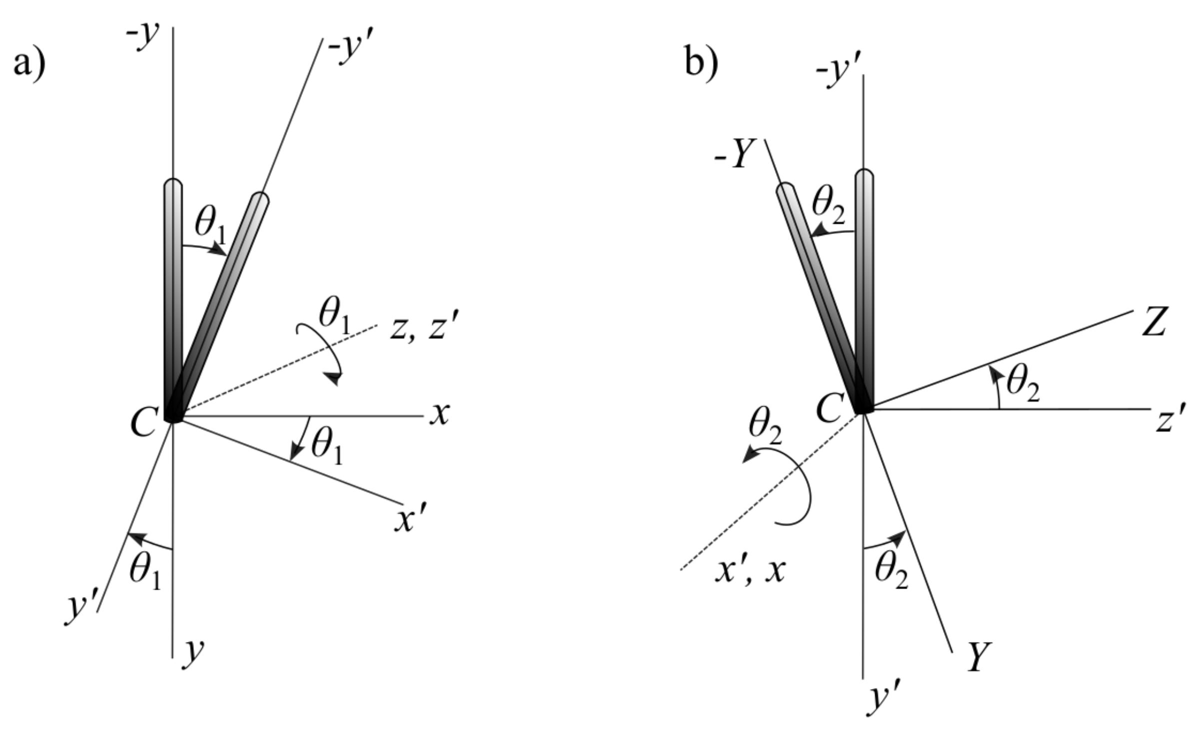
Consider the slender rod making point contact with the impact surface, shown in Figure 6. The impact and friction forces do not create a moment about the axis of the rod, so that we can bring the rod into position with two Euler angle rotations discussed earlier and depicted in Figure 7.
We select the first rotation to be by about the z axis, leading to the coordinates. The second rotation is about the axis by , leading to the coordinates. The transformation between the and coordinates is given by
where and
and use Equation (43) to calculate the inertia matrix about the fixed axes. This approach permits simulation of the impact equation for the full range of orientations.
When the coordinates of the center of mass of the impacting object is given, say, , we use these coordinates to calculate the orientation angles and . For a rod of length , noting that and that ,
The above equation gives three expressions to find two unknowns, and . The equations are consistent, with one unique solution. Note that when the body is not slender, three Euler angle rotations are necessary. Care must be taken when dealing with inverse sines and cosines, because of definition of their range in computer software. Once the two angles and are determined, the approach discussed above gives the inertia matrix.
We next outline a procedure to find the modes of impact. We assume that mass and inertia properties, initial orientation, initial velocities and initial angular velocities are known, as well as the coefficients of friction and restitution. The flowchart of the impact simulation is given in Figure 2. The only difference from two-dimensional impact is to replace the term reverse sliding with change in sliding direction in the flowchart.
- If sliding comes to an end during compression, split the compression stage into two periods, and , and check if the contact point sticks. Find associated sliding angle and use Equation (57) to calculate the impulsive forces. Use Equation (58) to check whether the available friction force is greater than friction necessary to prevent sliding. If so, the object will stick and continue sticking during restitution.If there is not sufficient friction, the object will reverse slide. Use Equations (51) and (53) with the appropriate superscripts to find the velocities after compression. Because the contact point C slides due to the effect of the moments generated by the orientation of the body, sliding will continue through restitution.
- If impact point has zero horizontal velocity before impact, check if impact point sticks using Equation (57). Find , and determine whether the amount of friction needed to sustain the no slip condition is less than the available friction. If there is not sufficient friction, the impact point will slide throughout compression and Equations (51) and (53) apply. This mode of motion continues through restitution.
At end of compression, the impact point may be sliding, reverse sliding, or sticking. We next consider restitution.
- If the impact point is sliding at end of compression, go through the same process as outlined in the compression stage to determine if sliding comes to an end or it continues. If sliding comes to an end, split the restitution stage into two periods and and check if the impact point sticks or slides in another direction. Use for Poisson and Equation (65) for the energetic model.If the sliding at end of compression is due to a mode change, so that there is reverse sliding, the changed mode will continue during restitution as well.
The impact equations in Equation (56) are nonlinear when motion comes to a rest (during compression or restitution) or when the energetic model is used to model restitution. Nonlinear equations usually have multiple solutions. We should always check if the numerical answers make sense. For example, if the normal force turns out to be negative, the results are invalid and the assumed mode of motion is incorrect. Furthermore, by selecting initial values for the velocities and forces in a way that reflects the geometry, we can ensure convergence of the nonlinear equation solver to the correct values. One way to do this is to obtain the solution to the impact equations in the absence of friction and use the results of this analysis to specify initial estimates of the variables to be solved.
5. Results: Impact of a Rod with the Ground
Consider impact of a cylindrical rod of length and radius r. Ends of the rod are assumed to be spherical to model impact as point-to-line. Furthermore, it is assumed the distance between the contact point and the center of mass remains constant during impact. The parameters of the rod are (same as the rod dimensions for the two-dimensional case so we can compare the results; otherwise the procedure applies to any three-dimensional object). We conduct simulations for different orientations of the rod during impact, as well as different values for the coefficients of friction and restitution.
The inertia matrix for a symmetric cylindrical rod using a body-attached frame is
We assume that impact forces do not create a moment about the symmetry axis of the rod.
We first simulate the impact equations for the following initial conditions: and for . Figure 8, which uses the Poisson model for restitution, shows the mode of impact, the normalized vertical velocity of the impact point, and the ratio of final energy to initial kinetic energy. Energy is calculated as . The results are symmetric for positive and negative values of (only the velocity in z-direction will have a different sign) so that the plots are for positive values of . This analysis is carried out for the range of initial orientations . The nature of the results does not change as the range of angles is increased.
As expected, the motion is dominated by sliding, with a small range of sticking (during compression and also in restitution), and reverse sliding for larger values of . When the rod is relatively upright (small values of ), the rod will slide and then stick. As the orientation angles become larger, reverse sliding and sliding in other directions begin to dominate the motion. Furthermore, energy lost during impact is highest for when sliding comes to an end during one of the stages of impact.
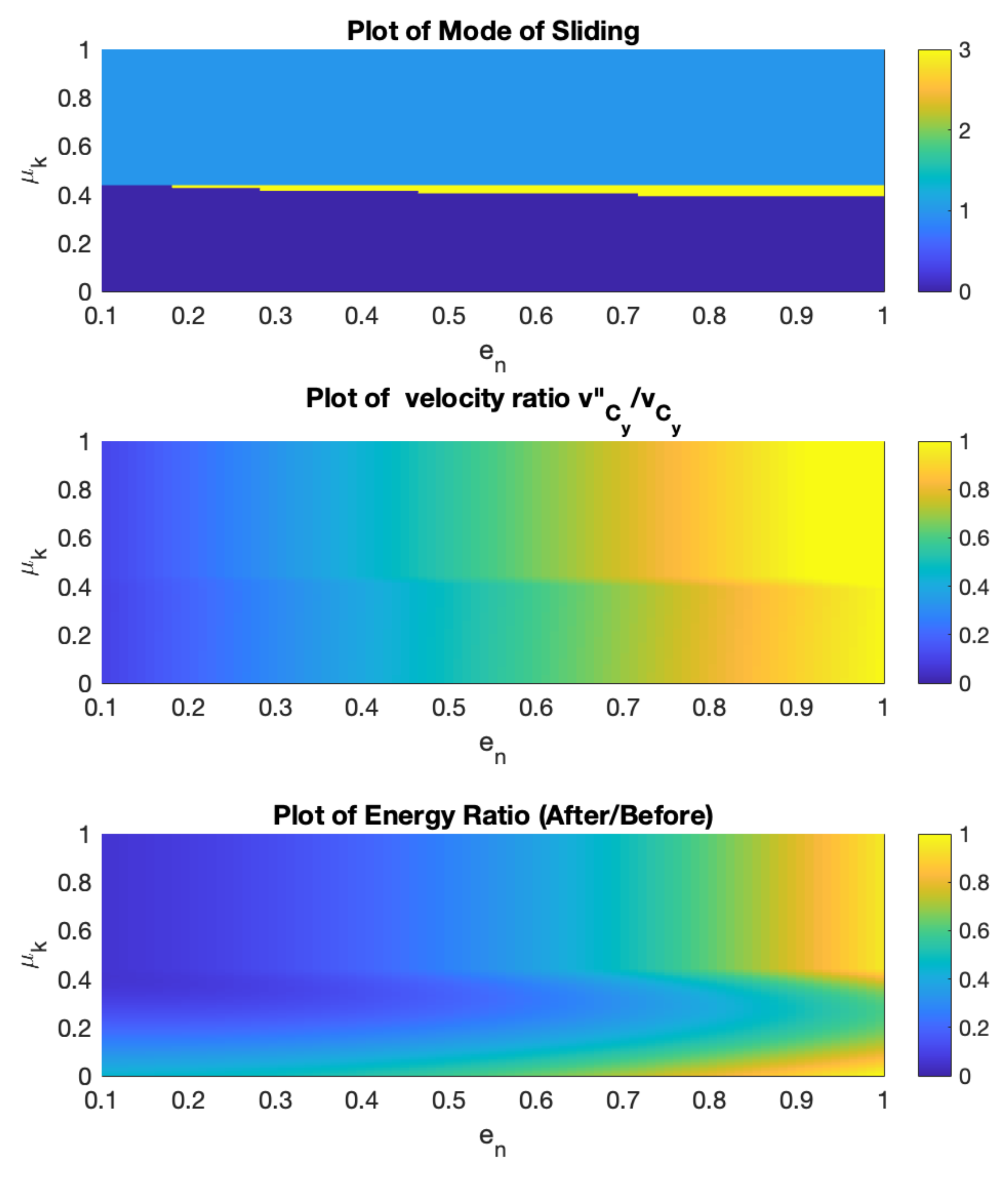
Next, let us consider the energetic coefficient of restitution and solve for the same initial conditions. The results are shown in Figure 9. Just as in the two-dimensional impact case, the results are very similar to Poisson’s model, with slight differences in only a few configurations.
For a parametric study, consider impact of a point mass with both a horizontal speed and vertical speed before impact. The impulsive normal force during compression is so that the horizontal impulsive friction force is approximated as . If this force is greater than the object will stop sliding. We then define a slide parameter ( for the rigid-body model) that relates the initial conditions and available friction. When , sliding will end, and when , sliding continues during compression. While the slide parameter is defined for particles, it can be used as a guideline for rigid body impact. For example, for the case considered above, , so that we can expect sliding to continue in one form or another for the majority of orientations.
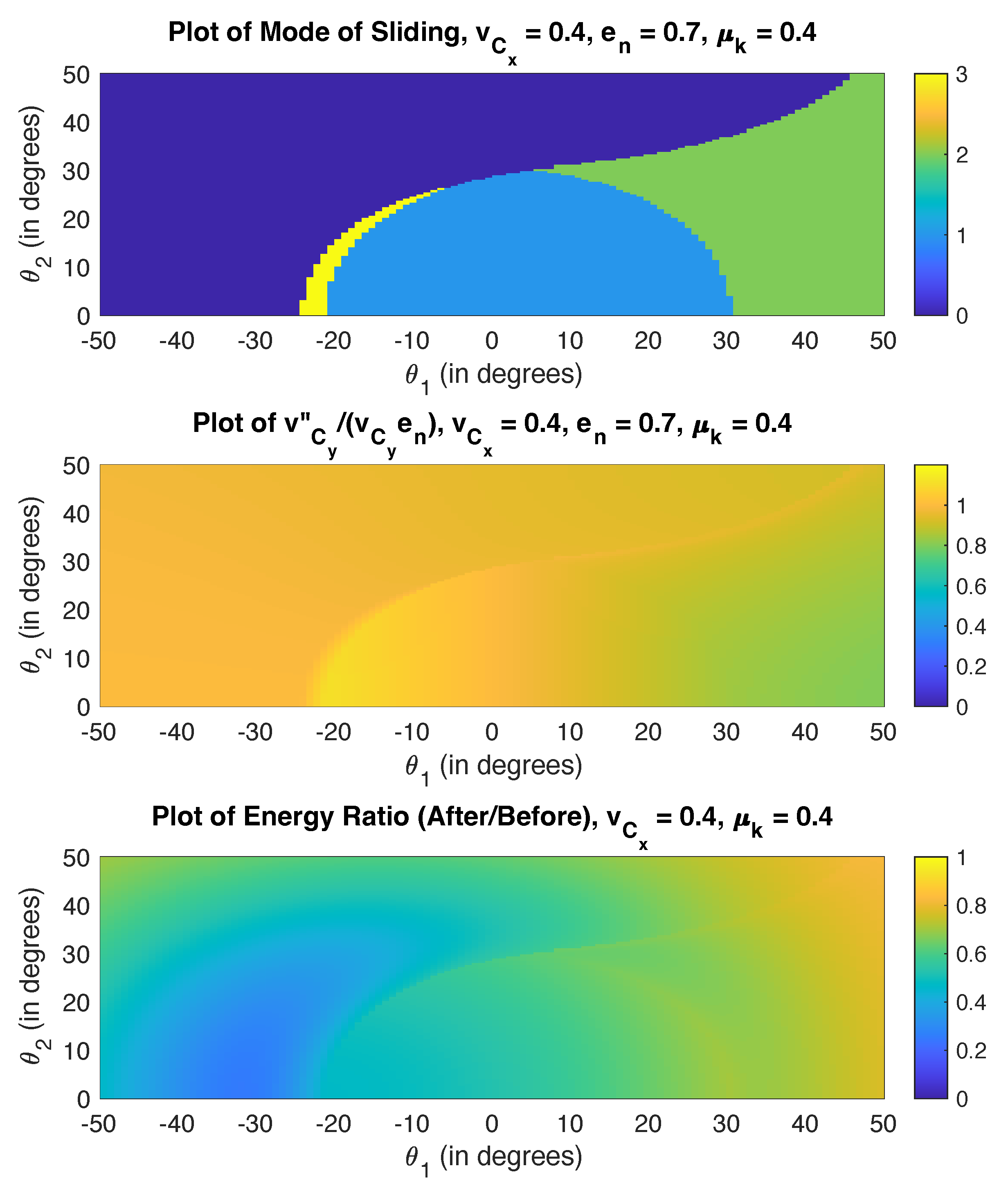
Let us consider a case when the slide parameter is close to one. Selecting leads to a slide parameter of . The results are shown in Figure 10 for Poisson’s model. The ranges for and are between and .
Here, the region when the rod sticks is larger than when . Furthermore, the parameters used here are the same as the ones in the two-dimensional example earlier (Figure 3 and Figure 4). Indeed, if we consider a line that represents a velocity ratio of 0.4 in the two-dimensional case and in the three-dimensional case, the results are the same.
We consider next the same initial conditions with and . The results are shown in Figure 11 using Poisson’s model.
Reduction in the coefficient of restitution increases energy loss, slightly affects velocity ratios (as they are normalized with respect to the coefficient of restitution), but does not affect the mode of motion, just as we observed in the two-dimensional results. Note there is no reverse sliding during restitution in any of the cases considered above.
We next analyze impact results as a function of the coefficients of friction and restitution. Using the same parameters for the rod as before, initial orientation of , , and initial velocities of , Figure 12 gives the mode of motion, vertical velocity ratios and energy ratios before and after impact. Poisson’s model is used to model the friction force. It should be noted that, for the set of parameters used here, the energetic method produces nearly identical results to the Poisson model.
As expected, the mode of motion is not affected by the value of the coefficient of restitution. Noting that an initial orientation of will lead to change of direction of horizontal velocity and possible reverse sliding, for low levels of friction the contact point continues sliding, albeit with change in direction. Even though reverse sliding is expected, friction is not sufficient to make sliding come to an end. However, the sliding direction, which initially was in the x-direction, acquires a component in the z-direction.
As friction increases, sliding comes to an end and reverse sliding in the negative x-direction begins. For high levels of friction, the impulsive friction force is sufficient to prevent reverse sliding and the contact point sticks. In our simulations, we found very few cases where, for a given level of friction, the mode of motion changes as is varied. The initial orientation is one such case and the results are plotted in Figure 13.
The vertical velocity ratio of the contact point is affected by both the coefficient of restitution and coefficient of friction. However, plays a much more significant factor. Note that, unlike previous figures, the velocity ratio is not normalized with respect to the coefficient of restitution. Similarly, the energy loss is influenced much more by than by . Noted that, in certain cases, the translational kinetic energy of the rod is converted into rotational kinetic energy.
6. Discussion
As in the case of two-dimensional impact, whether there is sliding or not is influenced more by the angle the rod makes with the vertical than the level of friction. When , because the rod is already sliding, sticking occurs in a smaller range of and . Therefore, there is more sliding and reverse sliding in three-dimensional impact, as sliding can occur perpendicular to the initial planar velocity.
As in two-dimensional impact, there is more energy loss as the coefficient of restitution is decreased, friction is increased, and also when the rod becomes more flat. We can observe these effects by looking at the right side of the energy ratio plots. Using a static coefficient of friction different than the kinetic coefficient of friction does not change the results in a significant way.
The Poisson and energetic models give similar results for the majority of initial conditions for both two- or three-dimensional impact, as we split the stage in which sliding ends into two periods. The mode of motion is not dependent on Poisson and energetic models. As in the two-dimensional case, the difference in vertical velocity and energy ratio for the two models is more pronounced when sliding comes to a rest during compression or restitution.
7. Conclusions
Post-impact parameters are analyzed for three-dimensional impact. A procedure is developed to approximate direction of the frictional forces along the impact plane. Simulations are conducted using both Poisson’s and energetic models. It is observed that the three-dimensional results follow closely from two-dimensional impact results, with more sliding observed for three-dimensional impact. The mode of impact is primarily influenced by friction and orientation of the body. It is not affected by the coefficient of restitution for two-dimensional impact and is affected minimally for three-dimensional impact. The velocity and energy ratios before and after impact are primarily affected by the coefficient of restitution. These two conclusions regarding coefficient of restitution apply to both the Poisson and energetic models. The Poisson and energetic models yield very similar results but, in a limited number of cases, there may be up to a 20% difference in post-impact velocities. A closed-form solution is developed for the modes of motion for two-dimensional impact.
Author Contributions
Conceptualization, H.S. and H.B.; methodology, H.S.; software, H.B.; validation, H.S., H.B.; formal analysis, H.S., H.B.; investigation, H.B.; resources, H.B.; data curation, H.S., H.B.; writing—original draft preparation, H.S., H.B.; writing—review and editing, H.B.; visualization, H.B.; supervision, H.B.; project administration, H.S., H.B.; funding acquisition, H.B. All authors have read and agreed to the published version of the manuscript.
Funding
Haim Baruh’s research was funded in part by the NASA Grant 80NSSC20M0066.
Institutional Review Board Statement
Not applicable.
Informed Consent Statement
Not applicable.
Acknowledgments
The authors would like to thank the two anonymous reviewers for their very valuable comments.
Conflicts of Interest
The authors declare no conflict of interest.
References
- Wang, Y.; Mason, M. Two-Dimensional Rigid-Body Collisions With Friction. J. Appl. Mech. 1992, 59, 635. [Google Scholar] [CrossRef]
- Stronge, W. Rigid body collisions with friction. Proc. R. Soc. Lond. Ser. A Math. Phys. Sci. 1990, 431, 169–181. [Google Scholar]
- Routh, E. The Advanced Part of a Treatise on the Dynamics of a System of Rigid Bodies; Cambridge University Press: Cambridge, UK, 1905. [Google Scholar]
- Stronge, W. Impact Mechanics; Cambridge University Press: Cambridge, UK, 2004. [Google Scholar]
- Whittaker, E. A Treatise on the Analytical Dynamics of Particles and Rigid Bodies with an Introduction to the Problem of Three Bodies; CUP Archive: Cambridge, UK, 1970. [Google Scholar]
- Brach, R. Rigid body collisions. J. Appl. Mech. 1989, 56, 133–138. [Google Scholar] [CrossRef]
- Brach, R. Formulation of rigid body impact problems using generalized coefficients. Int. J. Eng. Sci. 1998, 36, 61–71. [Google Scholar] [CrossRef]
- Brach, R. Mechanical Impact Dynamics: Rigid Body Collisions; Brach Engineering, LLC: Granger, IN, USA, 2007. [Google Scholar]
- Smith, C. Predicting rebounds using rigid-body dynamics. J. Appl. Mech. 1991, 58, 754–758. [Google Scholar] [CrossRef]
- Keller, J. Impact with friction. J. Appl. Mech. 1986, 53, 1–5. [Google Scholar] [CrossRef]
- Brogliato, B. Nonsmooth Mechanics, 3rd ed.; Springer: Berlin/Heidelberg, Germany, 2016. [Google Scholar]
- Mac Sithigh, G. Rigid-body impact with friction-various approaches compared. ASME Appl. Mech. Div.-Publ. 1995, 205, 307. [Google Scholar]
- Brake, M. The effect of the contact model on the impact-vibration response of continuous and discrete systems. J. Sound Vib. 2013, 332, 3849–3878. [Google Scholar] [CrossRef]
- Rigaud, E.; Perret-Liaudet, J. Experiments and numerical results on non-linear vibrations of an impacting Hertzian contact. Part 1: Harmonic excitation. J. Sound Vib. 2003, 265, 289–307. [Google Scholar] [CrossRef] [Green Version]
- Wu, S.; Yang, S.; Haug, E. Dynamics of mechanical systems with Coulomb friction, stiction, impact and constraint addition-deletion. Mech. Mach. Theory 1986, 21, 417–425. [Google Scholar] [CrossRef]
- Khulief, Y.; Shabana, A. Impact responses of multi-body systems with consistent and lumped masses. J. Sound Vib. 1986, 104, 187–207. [Google Scholar] [CrossRef]
- Yigit, A.; Ulsoy, A.; Scott, R. Dynamics of a radially rotating beam with impact. I: Theoretical and computational model. J. Vib. Acoust. Stress. Reliab. Des. 1990, 112, 65–70. [Google Scholar] [CrossRef]
- Jia, Y. Energy-Based Modeling of Tangential Compliance in 3-Dimensional Impact. In Algorithmic Foundations of Robotics IX; Springer: Berlin/Heidelberg, Germany, 2011; pp. 267–284. [Google Scholar]
- Jia, Y. Three-dimensional impact: Energy-based modeling of tangential compliance. Int. J. Robot. Res. 2013, 32, 56–83. [Google Scholar] [CrossRef]
- Zhao, Z.; Liu, C.; Brogliato, B. Planar dynamics of a rigid body system with frictional impacts. II. Qualitative analysis and numerical simulations. Proc. R. Soc. A Math. Phys. Eng. Sci. 2009, 465, 2267–2292. [Google Scholar] [CrossRef] [Green Version]
- Wang, L.; Zhou, W.; Ding, Z.; Li, X.; Zhang, C. Experimental determination of parameter effects on the coefficient of restitution of differently shaped maize in three-dimensions. Powder Technol. 2015, 284, 187–194. [Google Scholar] [CrossRef]
- Zhan, L.; Peng, C.; Zhang, B.; Wu, W. Three-dimensional modeling of granular flow impact on rigid and deformable structures. Comput. Geotech. 2019, 112, 257–271. [Google Scholar] [CrossRef]
- Preclik, T.; Eibl, S.; Rude, U. The maximum dissipation principle in rigid-body dynamics with inelastic impacts. Comput. Mech. 2018, 62, 81–96. [Google Scholar] [CrossRef] [Green Version]
- Zhen, Z.; Liu, C. The analysis and simulation for three-dimensional impact with friction. Multibody Syst. Dyn. 2007, 18, 511–530. [Google Scholar] [CrossRef]
- Batlle, A. Rough balanced collision. ASME J. Appl. Mech. 1996, 23, 168–172. [Google Scholar] [CrossRef]
- Djerassi, S. Three-dimensional, one-point collision with friction. Multibody Syst. Dyn. 2012, 27, 173–195. [Google Scholar] [CrossRef]
- Stronge, W.J. Energetically consistent calculations for oblique impact in unbalanced systems with friction. ASME J. Appl. Mech. 2015, 82, 081003. [Google Scholar] [CrossRef]
- Sun, H. Three-Dimensional Rigid-Body Impact with Friction. Ph.D. Thesis, Rutgers, The State University of New Jersey, Piscataway, NJ, USA, 2017. [Google Scholar]
Figure 1.
Free body diagram of 2D model during impact assuming for .
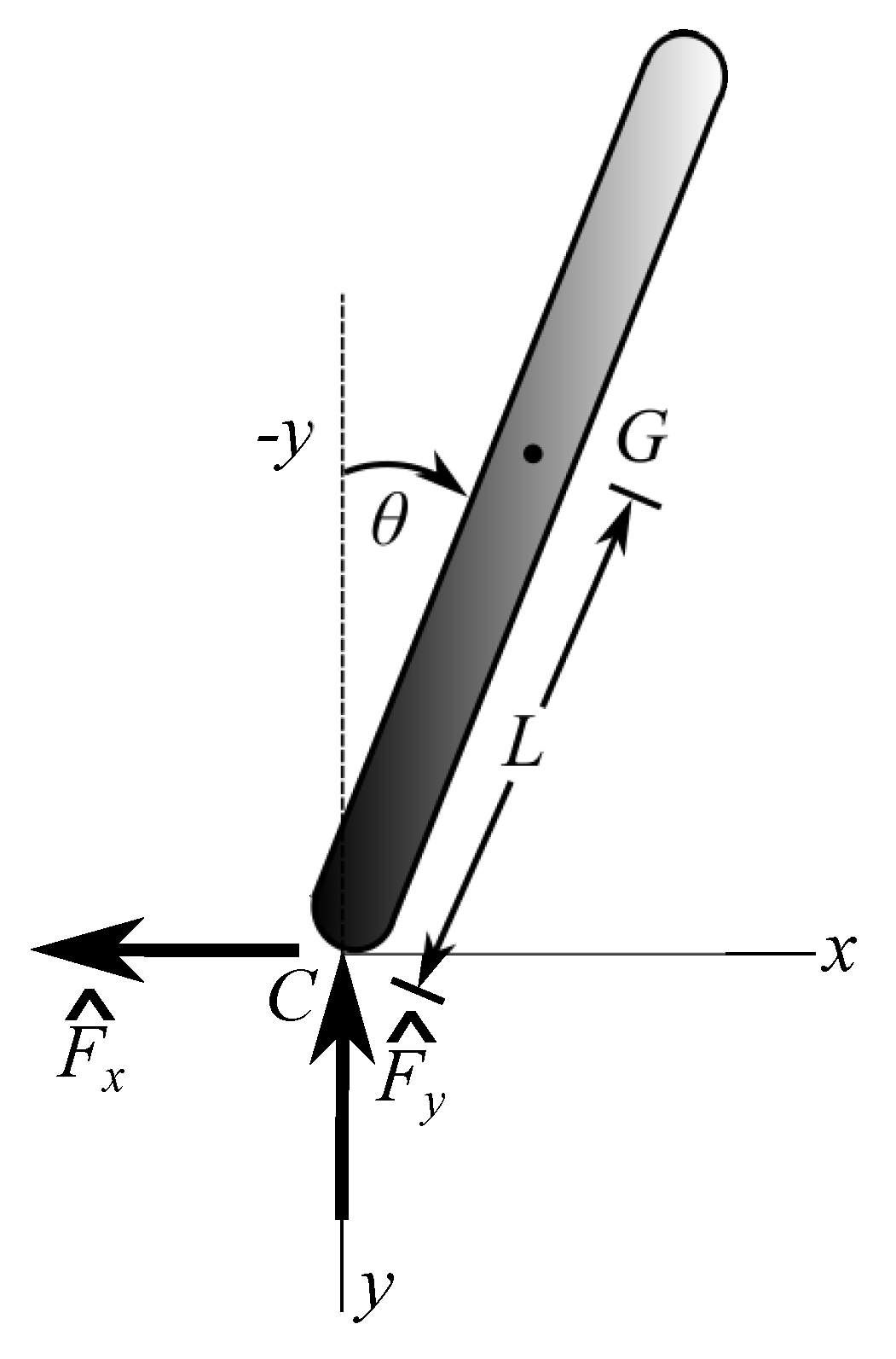
Figure 2.
Flowchart of simulation of impact for both 2D and 3D.
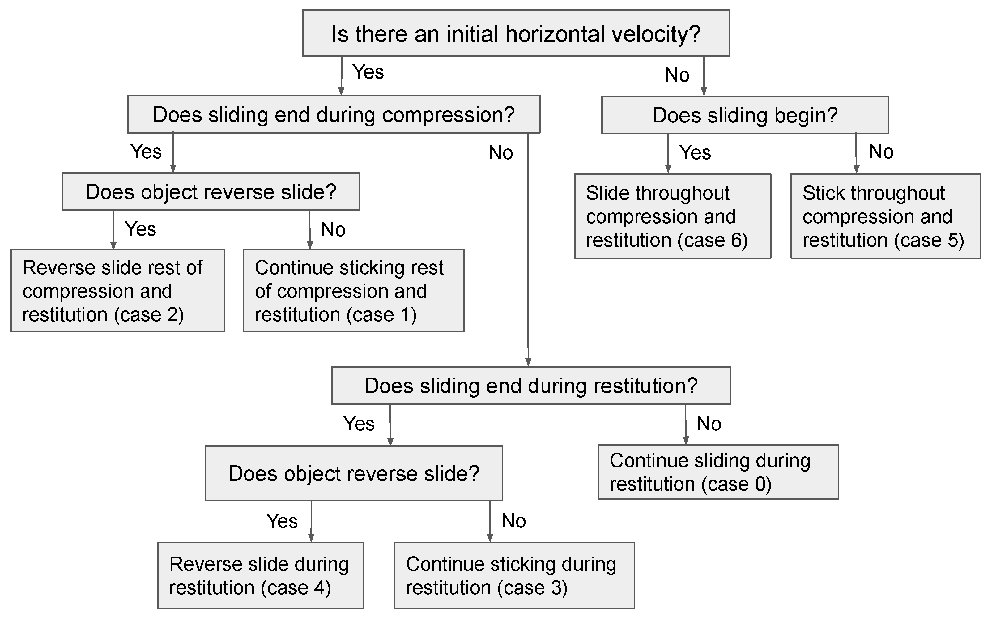
Figure 3.
Influence of orientation angle and velocity ratio on the type of impact for , , . Top figure: mode of sliding, middle figure: . Lower figure: energy ratio (after impact/before impact). Poisson’s model is used.
Figure 3.
Influence of orientation angle and velocity ratio on the type of impact for , , . Top figure: mode of sliding, middle figure: . Lower figure: energy ratio (after impact/before impact). Poisson’s model is used.
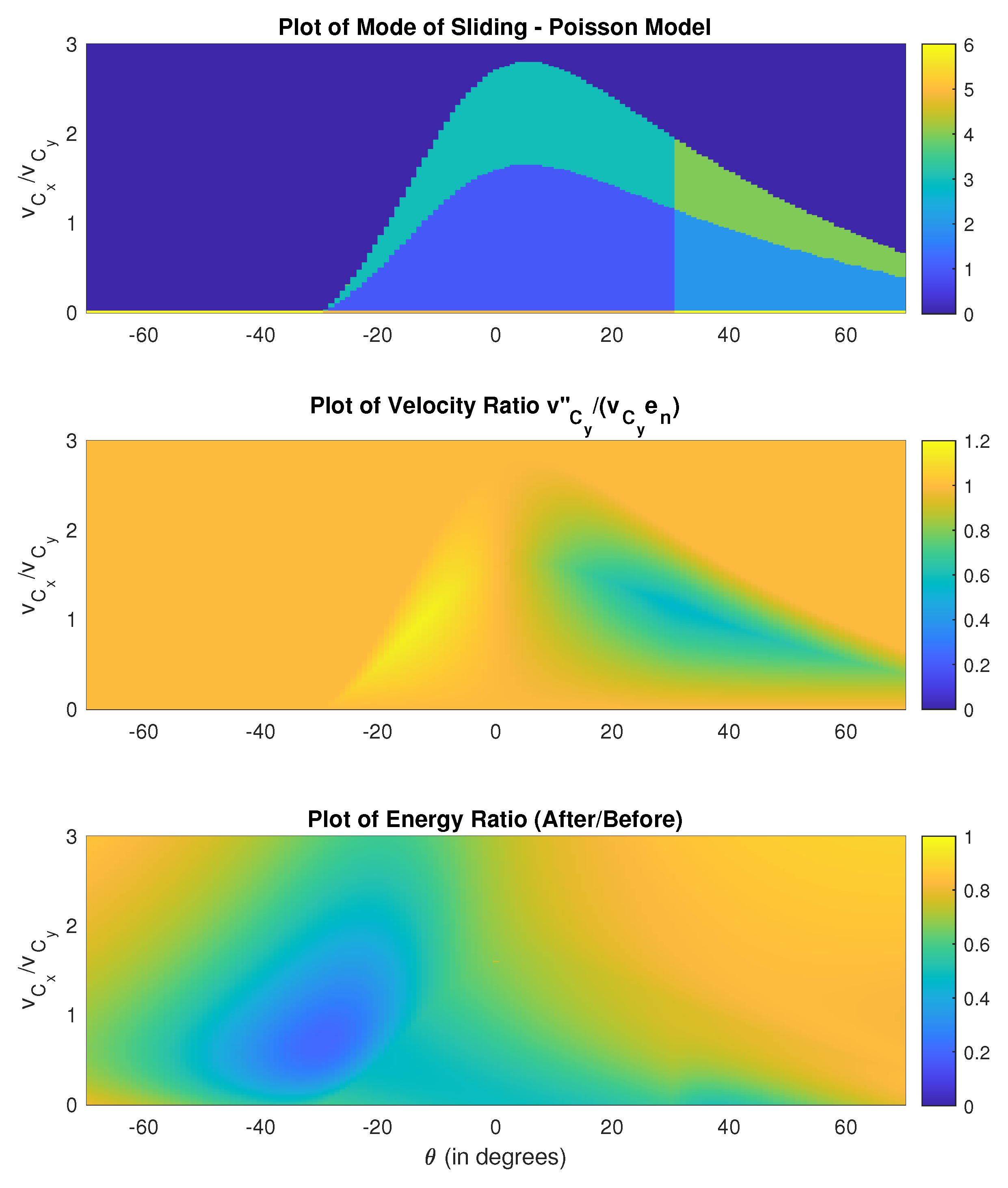
Figure 4.
Influence of orientation angle and velocity ratio on the type of impact for , , . Top figure: . Lower figure: energy ratio (after impact/before impact). Energetic coefficient of restitution is used.
Figure 4.
Influence of orientation angle and velocity ratio on the type of impact for , , . Top figure: . Lower figure: energy ratio (after impact/before impact). Energetic coefficient of restitution is used.
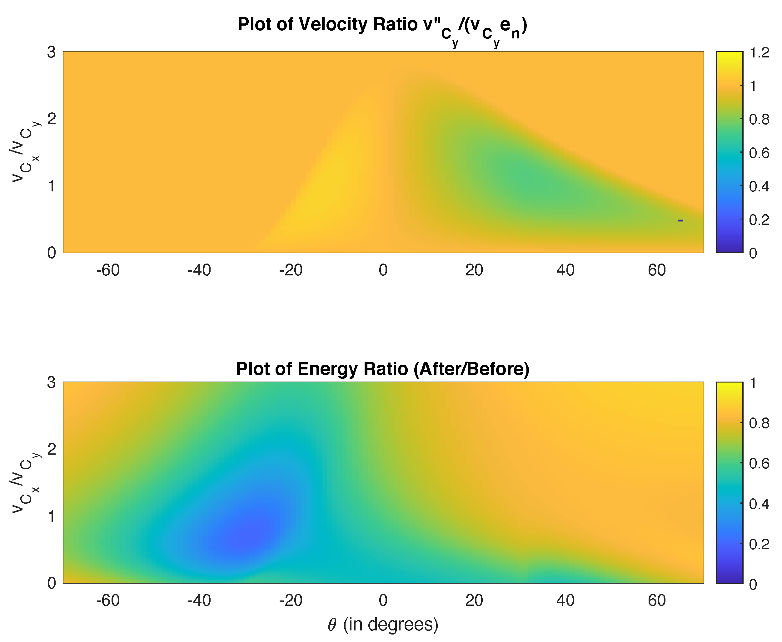
Figure 5.
Ratios of vertical velocity of impact point and energy left in system. Results for Poisson model divided by results obtained using the energetic model.
Figure 5.
Ratios of vertical velocity of impact point and energy left in system. Results for Poisson model divided by results obtained using the energetic model.
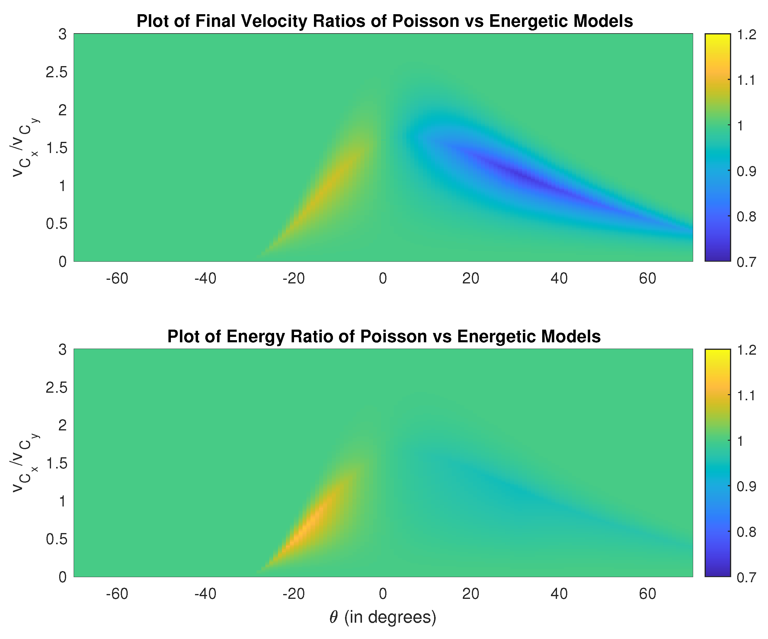
Figure 6.
Falling rod colliding with ground in three dimensions.
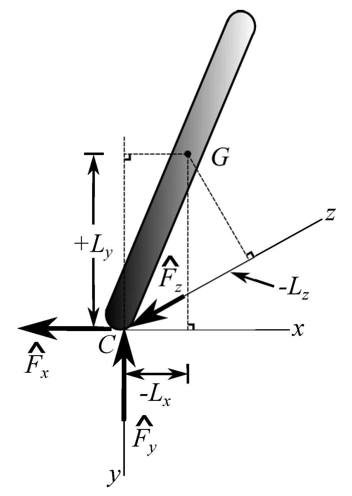
Figure 7.
Rotation angles (a) and (b) for a slender rod.

Figure 8.
Impact results for , using Poisson model.
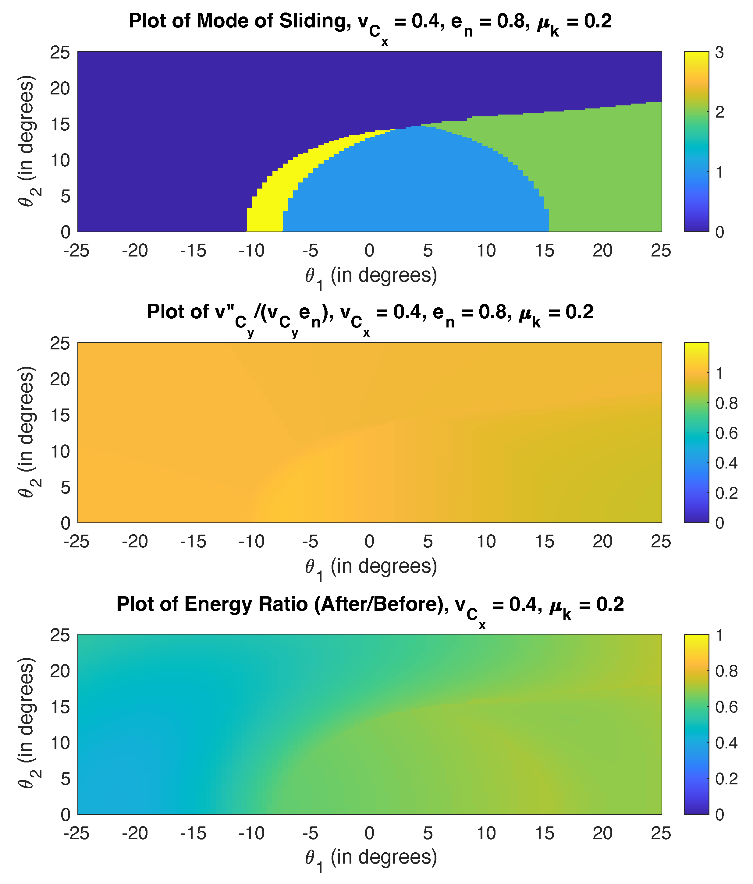
Figure 9.
Impact results for , using energetic coefficient of restitution.

Figure 10.
Impact results for , . Slide parameter is . Poisson’s model is used.

Figure 11.
Impact results for , . Poisson’s model is used.
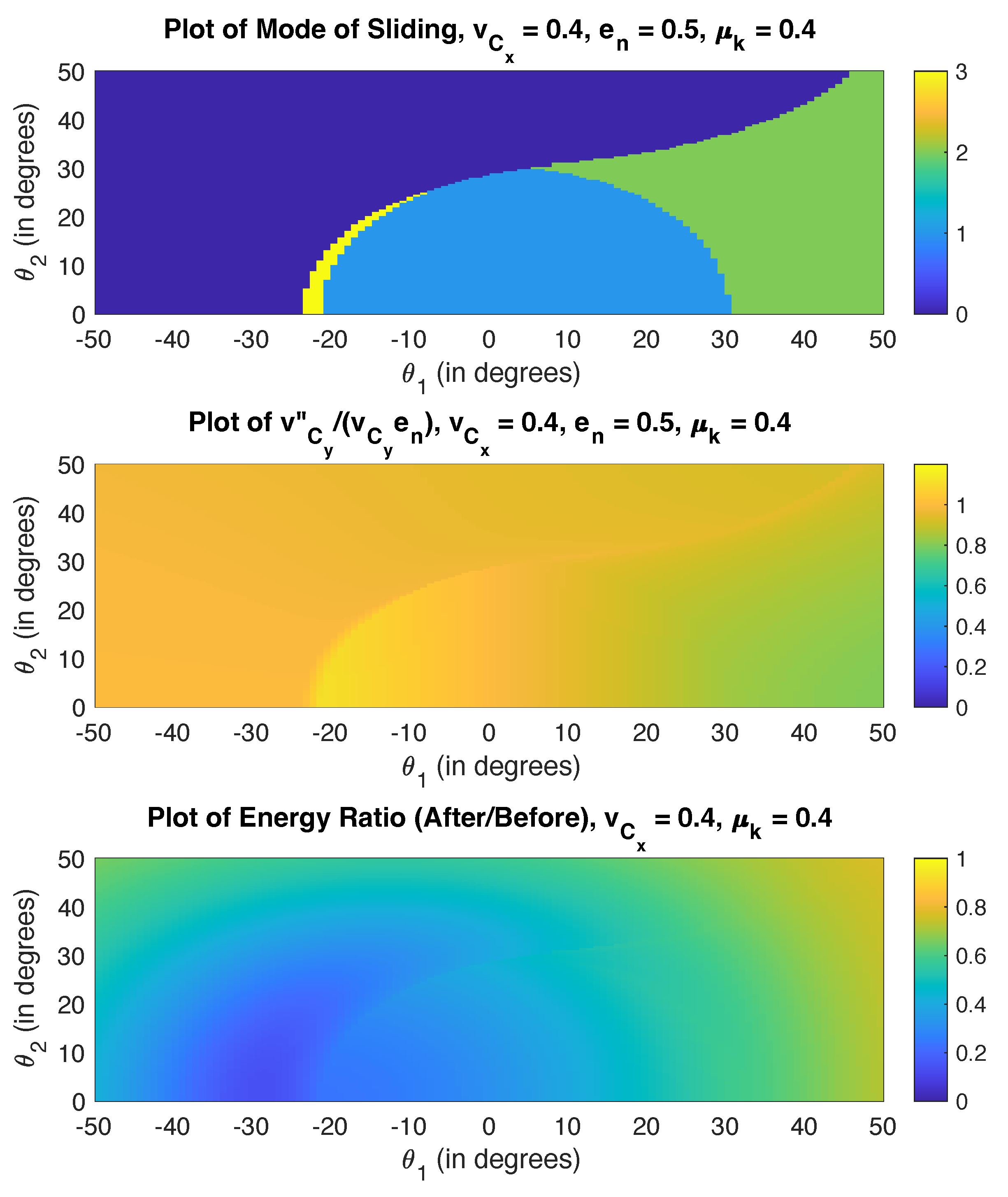
Figure 12.
Impact results as a function of and for .
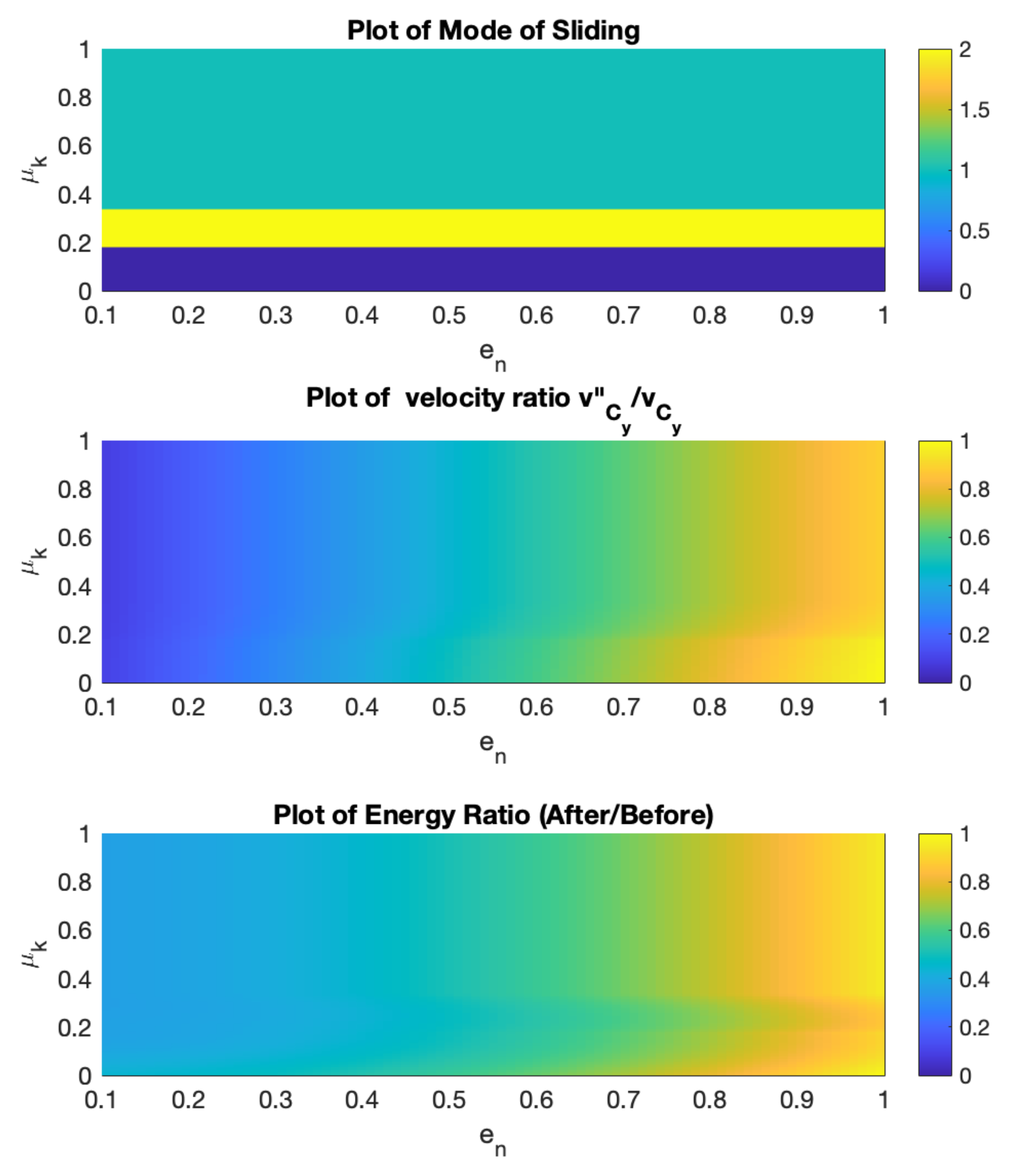
Figure 13.
Impact results as a function of and for .

Table 1.
Cases for two-dimensional (also three-dimensional) impact.
| Case | Initial | Compression | Restitution |
|---|---|---|---|
| No. | Condition | Stage | Stage |
| 0 | Sliding | Sliding | |
| 1 | Sliding ends, sticking | Sticking | |
| 2 | Sliding ends, reverse sliding | Reverse sliding | |
| 3 | Sliding | Sliding ends, sticking | |
| 4 | Sliding | Sliding ends, reverse sliding | |
| 5 | Sticking | Sticking | |
| 6 | Sliding | Sliding |
Table 2.
Stick-slide conditions based on ratios (for ).
| If | and Is | During Compression | During Restitution |
|---|---|---|---|
| any value | Sliding | Sliding | |
| and | Sliding | Sliding ends, sticking | |
| and | Sliding | Sliding ends, reverse sliding | |
| Sliding ends, sticking | Sticking | ||
| Sliding ends, reverse sliding | Reverse sliding | ||
| Sticking | Sticking | ||
| Sliding | Sliding |
Publisher’s Note: MDPI stays neutral with regard to jurisdictional claims in published maps and institutional affiliations. |
© 2022 by the authors. Licensee MDPI, Basel, Switzerland. This article is an open access article distributed under the terms and conditions of the Creative Commons Attribution (CC BY) license (https://creativecommons.org/licenses/by/4.0/).
Share and Cite
MDPI and ACS Style
Sun, H.; Baruh, H. Analysis of Three-Dimensional Rigid-Body Impact with Friction. Dynamics 2022, 2, 1-26. https://doi.org/10.3390/dynamics2010001
AMA Style
Sun H, Baruh H. Analysis of Three-Dimensional Rigid-Body Impact with Friction. Dynamics. 2022; 2(1):1-26. https://doi.org/10.3390/dynamics2010001
Chicago/Turabian StyleSun, Han, and Haim Baruh. 2022. "Analysis of Three-Dimensional Rigid-Body Impact with Friction" Dynamics 2, no. 1: 1-26. https://doi.org/10.3390/dynamics2010001