
Strain Gradient Theory Based Dynamic Mindlin-Reissner and Kirchhoff Micro-Plates with Microstructural and Micro-Inertial Effects


Abstract
1. Introduction
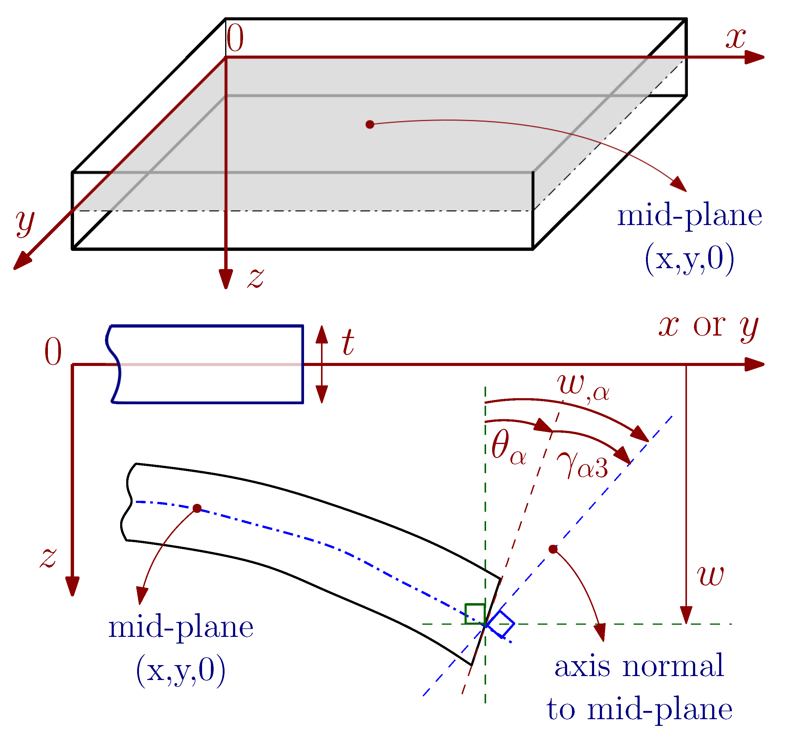
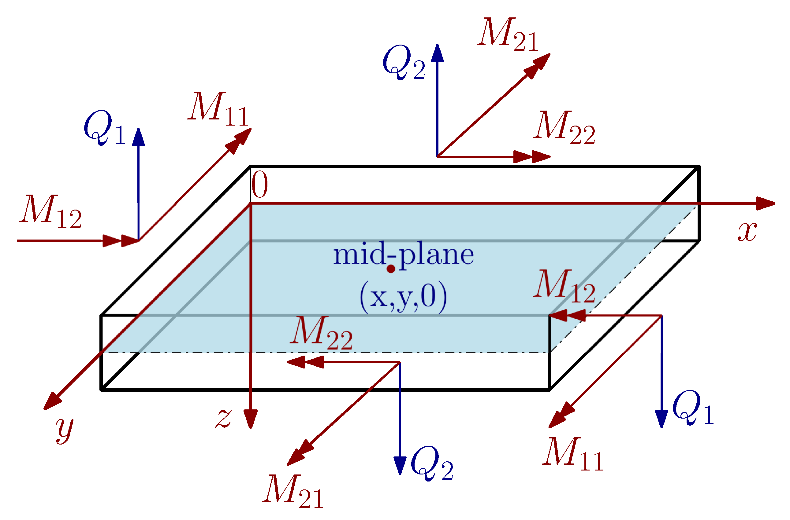
2. Basic Assumptions and Constitutive Relations for Grade-2 Mindlin–Reissner-Type Elastic Plates
3. Theoretical Basis for Mindlin–Reissner-Type Elastic Plates
4. Variational Formulation of Mindlin–Reissner-Type Gradient Elastic Plates
4.1. The Virtual Work of the Internal Forces
4.2. The Virtual Work of the Inertia Forces
4.3. The Virtual Work of the External Forces
4.4. The Governing Equations of Motion and the Boundary Conditions
4.5. Governing Equations of Motion and Boundary Conditions for Mindlin–Reissner-Type Strain Gradient Plate with Straight Boundaries Aligned to Axes x or y
5. Development of the Kirchhoff-Type Gradient Elastic Plate
5.1. The Virtual Work of the Internal Forces
5.2. The Virtual Work of the Inertia Forces
5.3. The Virtual Work of the External Forces
5.4. The Euler–Lagrange Equations of Motion and the Respective Boundary Conditions for Kirchhoff Type Gradient Elastic Plate
5.5. Governing Equation of Motion and Boundary Conditions for Kirchhoff Type Strain Gradient Plate with Straight Boundaries Aligned to x or y
6. Short Literature Review of Micro-Structured Plate Theories
6.1. Model M2: The Classical Mindlin–Reissner Plate
6.2. Model M3: S. Ramezani’s Mindlin Type Micro-Plate
6.3. Model M4: Modified Couple-Stress Mindlin Plate
6.4. Model M5: Non-Local Mindlin Elastic Plate
6.5. Model K1: Strain Gradient Kirchhoff Type Elastic Plate
6.6. Model K2: The Classical Kirchhoff Plate
6.7. Model K3: Papargyri-Beskou’s Gradient Kirchhoff Type Elastic Plate
6.8. Model K4: Modified Couple-Stress Kirchhoff Type Elastic Plate
6.9. Model K5: Non-Local Kirchhoff Elastic Plate
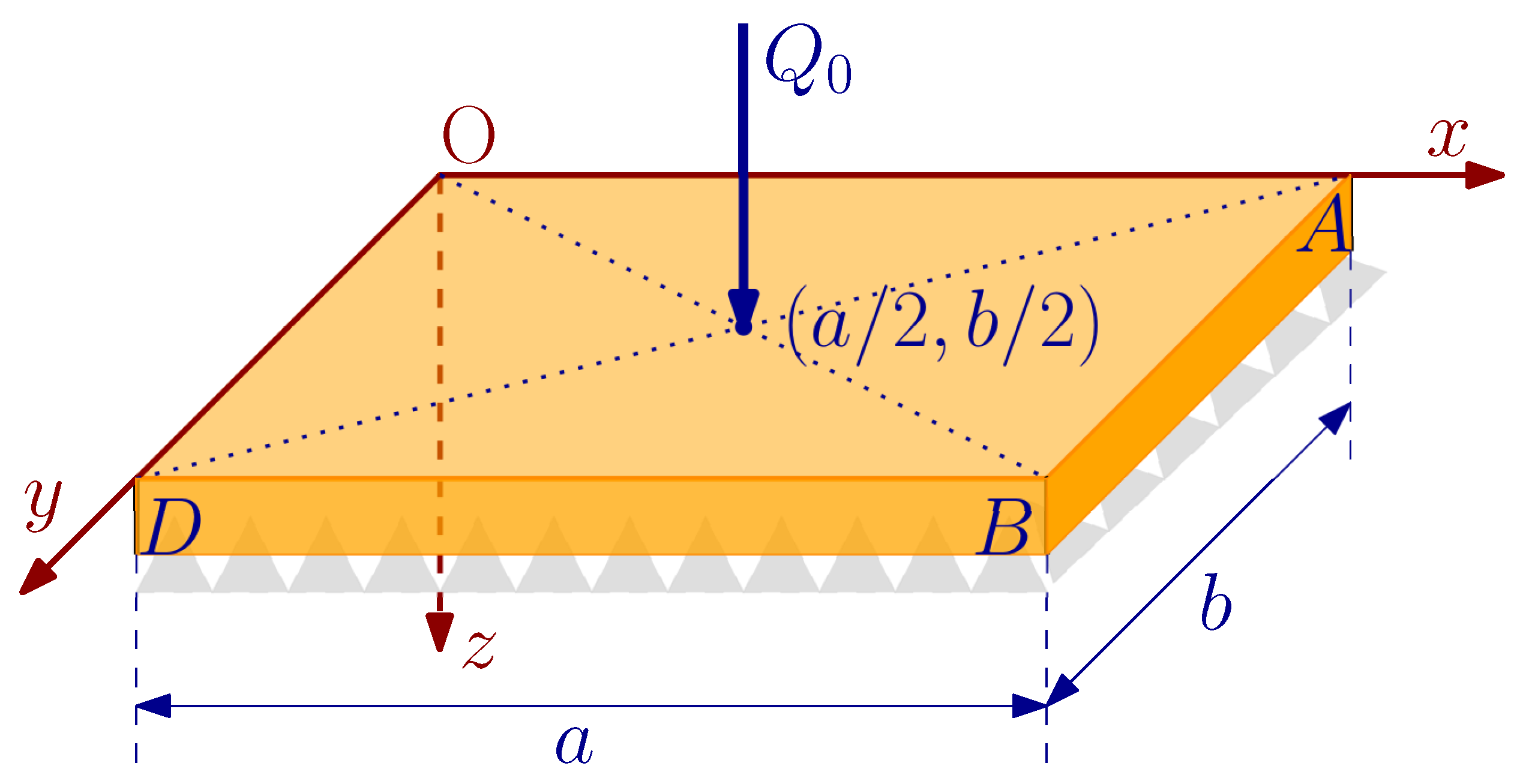
7. Example: Navier Solutions for Static Bending and Free Vibration of a Simply Supported Rectangular Plate
7.1. Boundary Conditions for the Mindlin–Reissner Plate Model M1
7.2. Boundary Conditions for the Kirchhoff Plate Model K1
7.3. Boundary Conditions for the Classical Mindlin–Reissner Plate Model M2
7.4. Boundary Conditions for the Classical Kirchhoff Plate Model K2
7.5. Static Bending Behavior for Mindlin–Reissner Plate Model M1
7.6. Free Vibration Behavior for Mindlin–Reissner Plate Model M1
7.7. Static Bending and Free Vibration Behavior for Kirchhoff Plate Model K1
- (1)
- for the static bending problem the bending Fourier coefficients are given as
- (2)
- while, for the free vibration problem the flexural fundamental frequencies are obtained,
8. Numerical Results and Comparison between Models
8.1. Numerical Results for the Static Bending Problem
8.1.1. Influence of Strain Gradient Effect on Thin Plates
8.1.2. Influence of Strain Gradient Effect on Thick Plates
8.2. Free Vibration Problem
8.2.1. Natural Frequencies for Mindlin–Reissner Type Plate Models
8.2.2. Natural Frequencies for Kirchhoff Type Plate Models
8.2.3. Comparison of Natural Frequencies between Mindlin-Type (M1) and Kirchhoff-Type (K1) Plate Models
9. Summary and Conclusions
9.1. Conclusions for Static Bending Response of Micro-Plates
- The strain gradient effect is proved to be more significant when the plate thickness t is at the micron-scale. That said, for small ratios , models M1 and K1 are much stiffer than their classical counterparts, models M2 and K2, respectively, i.e., the deflection and the rotations are smaller than those predicted by models M2 and K2. These observations hold true for thick and thin plates, i.e., for every value of the ratio .
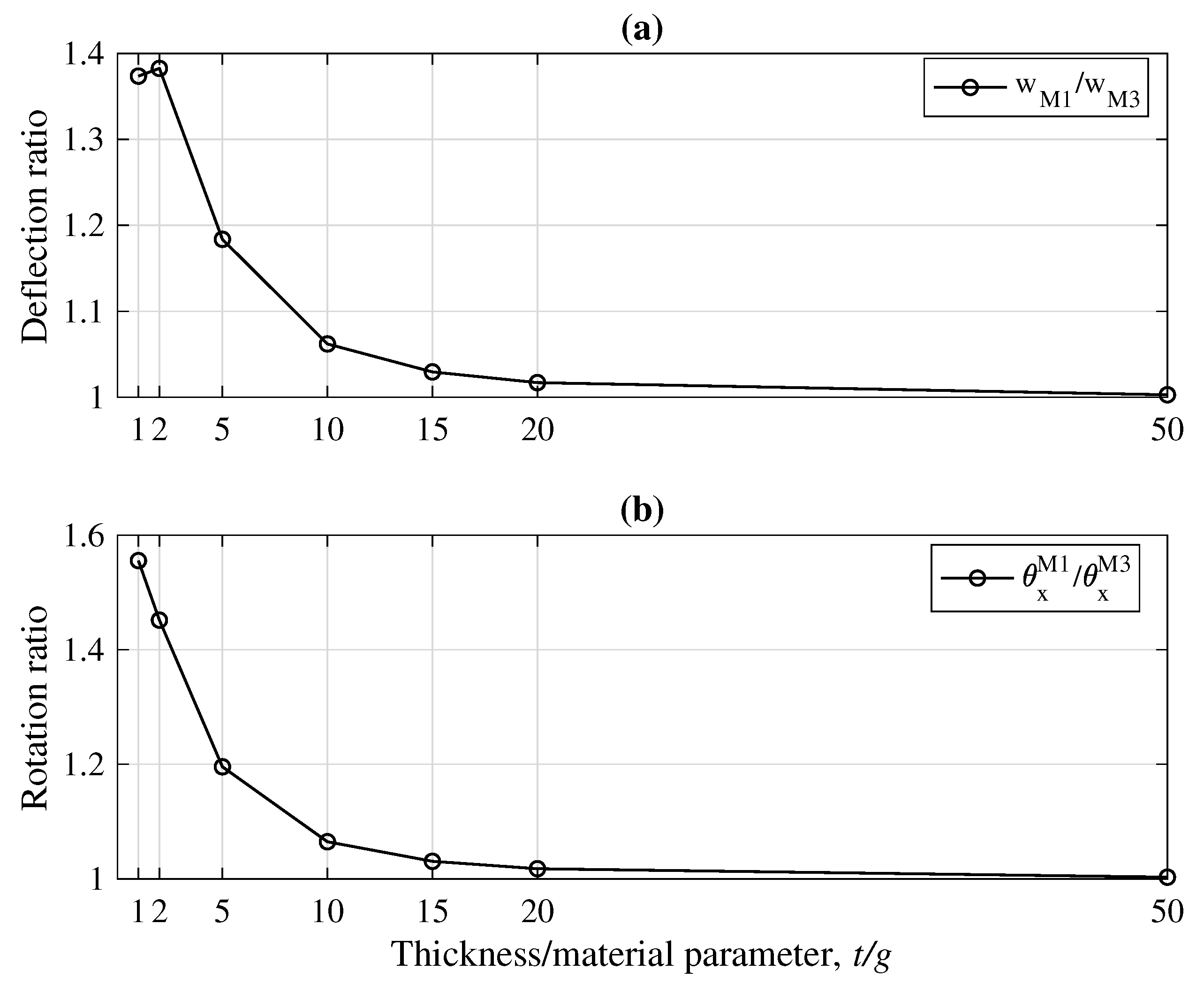
- Considering models M1 (present) and M3 (Ramezani’s), which were based on different plane stress assumptions (see Section 2 and Section 6.2), it is observed from Figure 8 that M1 is less stiff than M3, especially for small ratios . The two models converge for increasing values of the ratio .
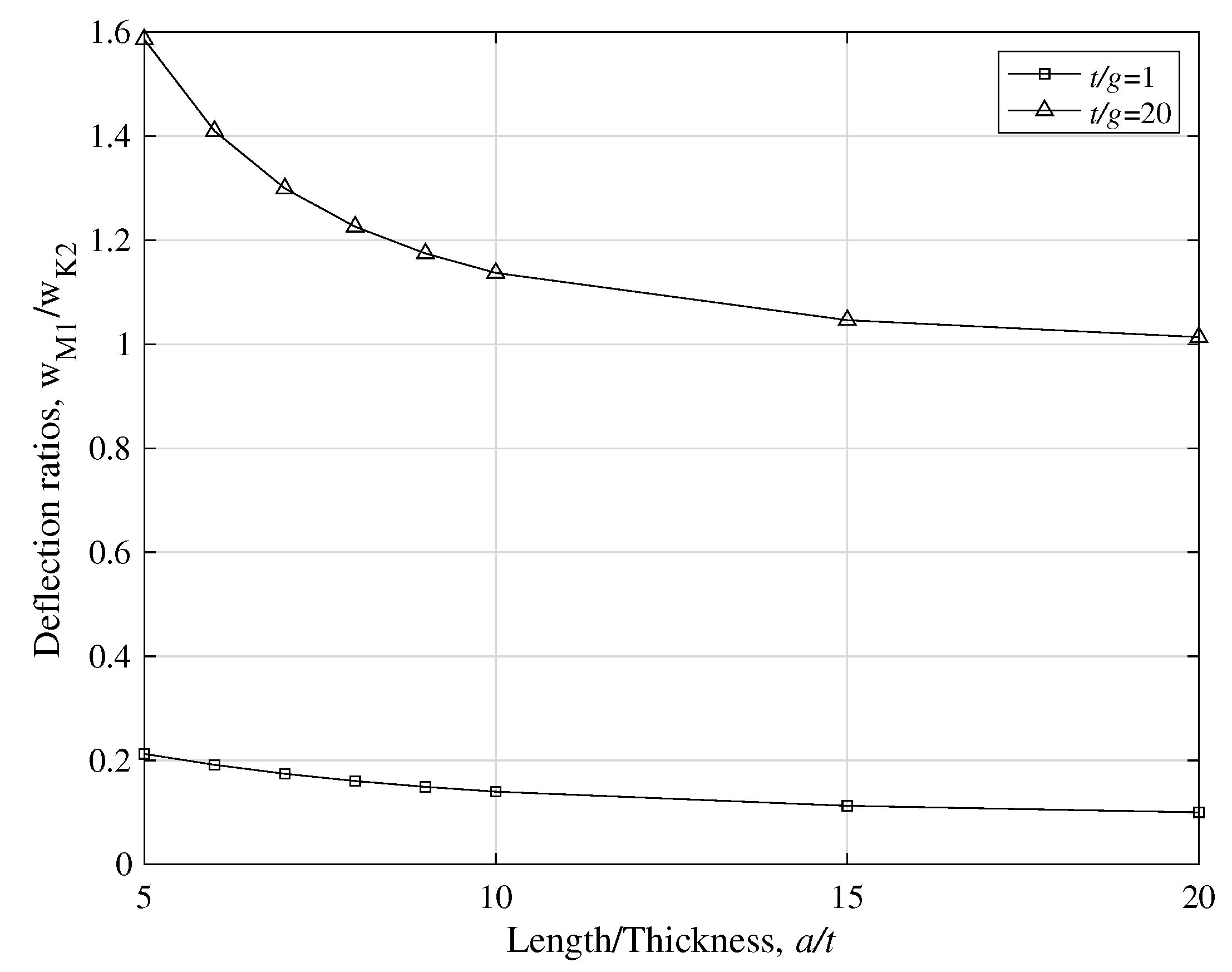
- Considering models M1 and K2, and Figure 11, the combined influence of the shear effect (characteristic of Mindlin–Reissner plates) and the strain gradient effect was investigated. For small ratios and in every range of ratio (i.e. for thick and thin plates), this combination is dominant and the two models deviate significantly from each other. For larger values of , the difference between the two models is important only for thick plates, while for thin plates ( or more) the two models converge, showing that the shear effect and the strain gradient effect diminish.
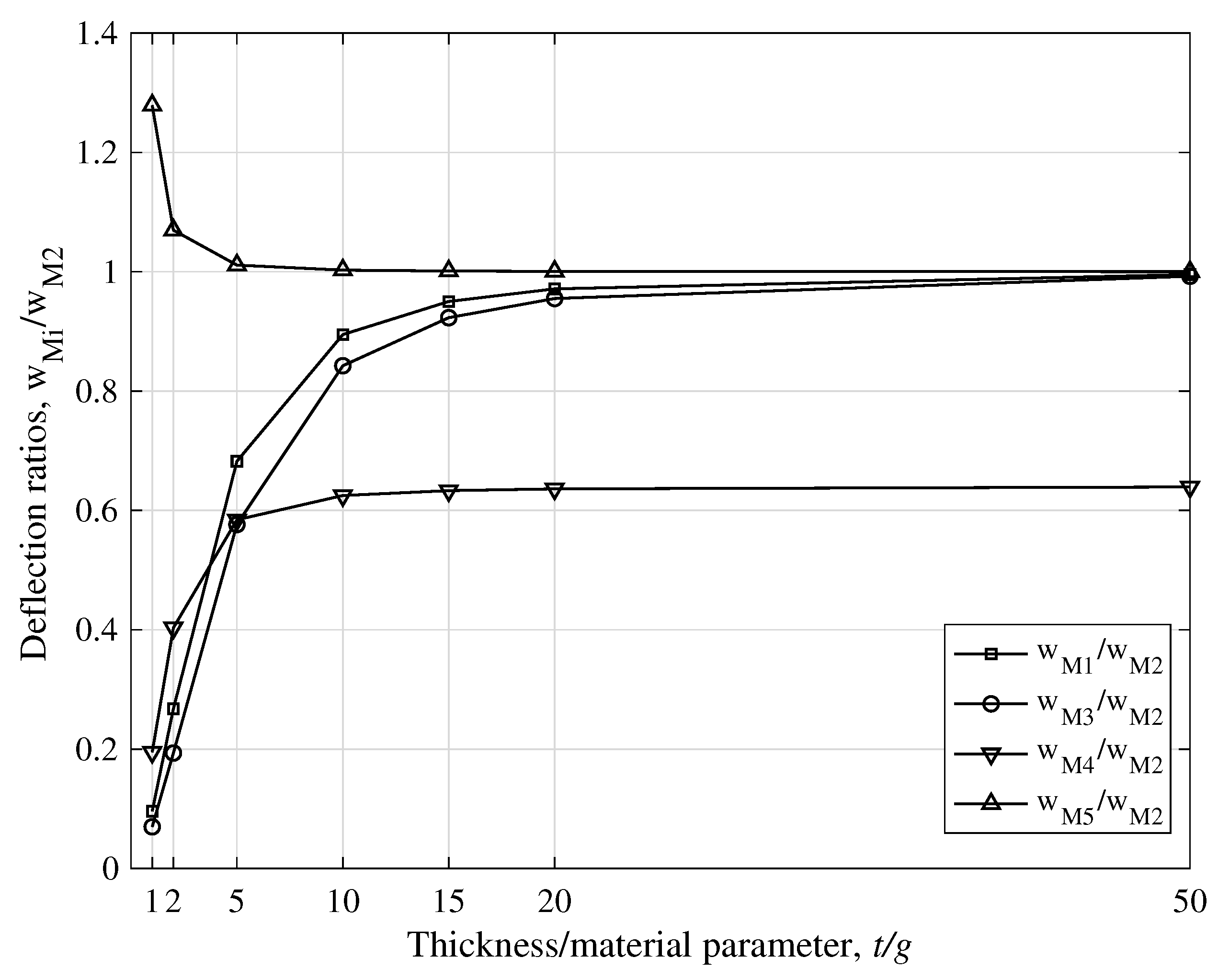
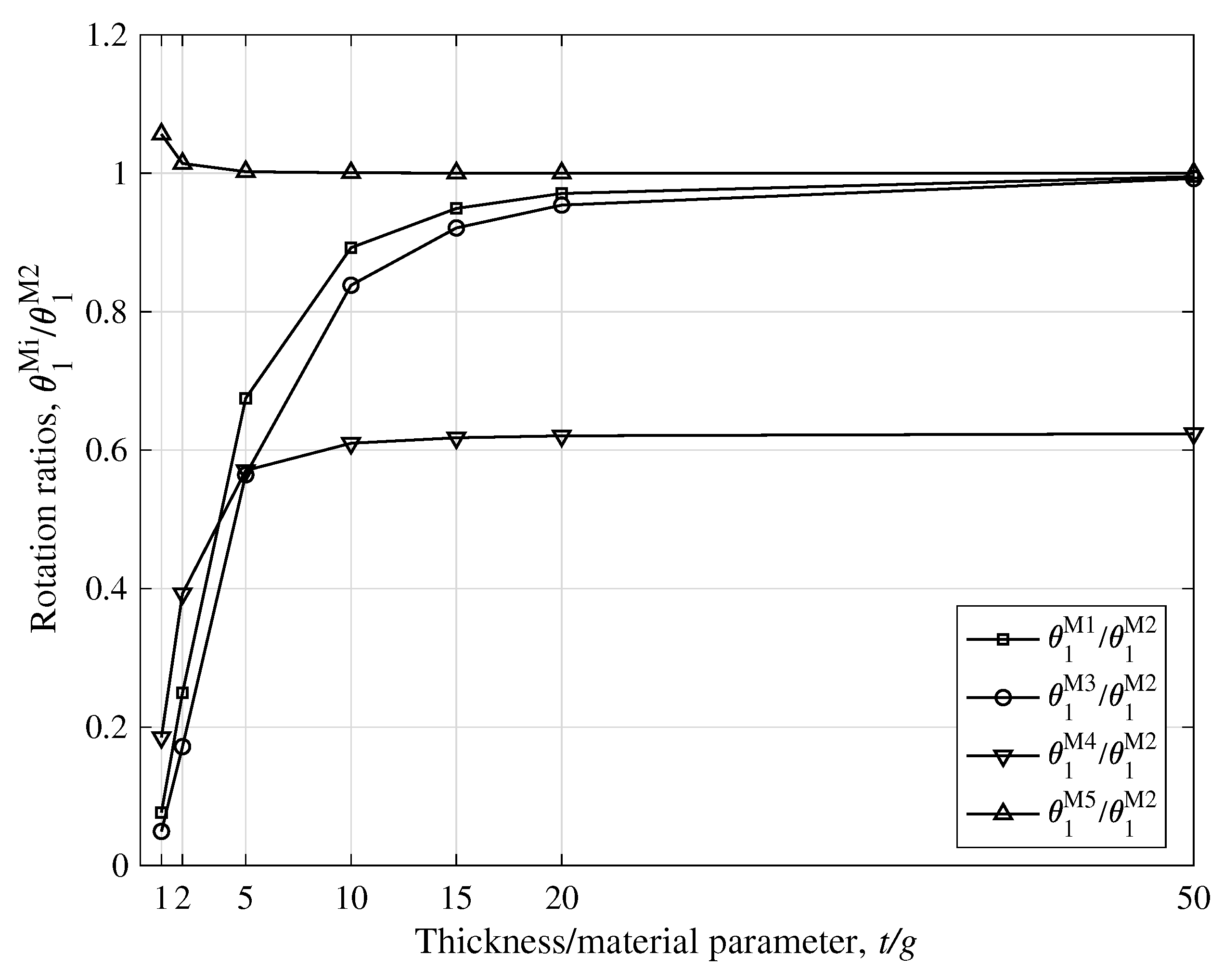
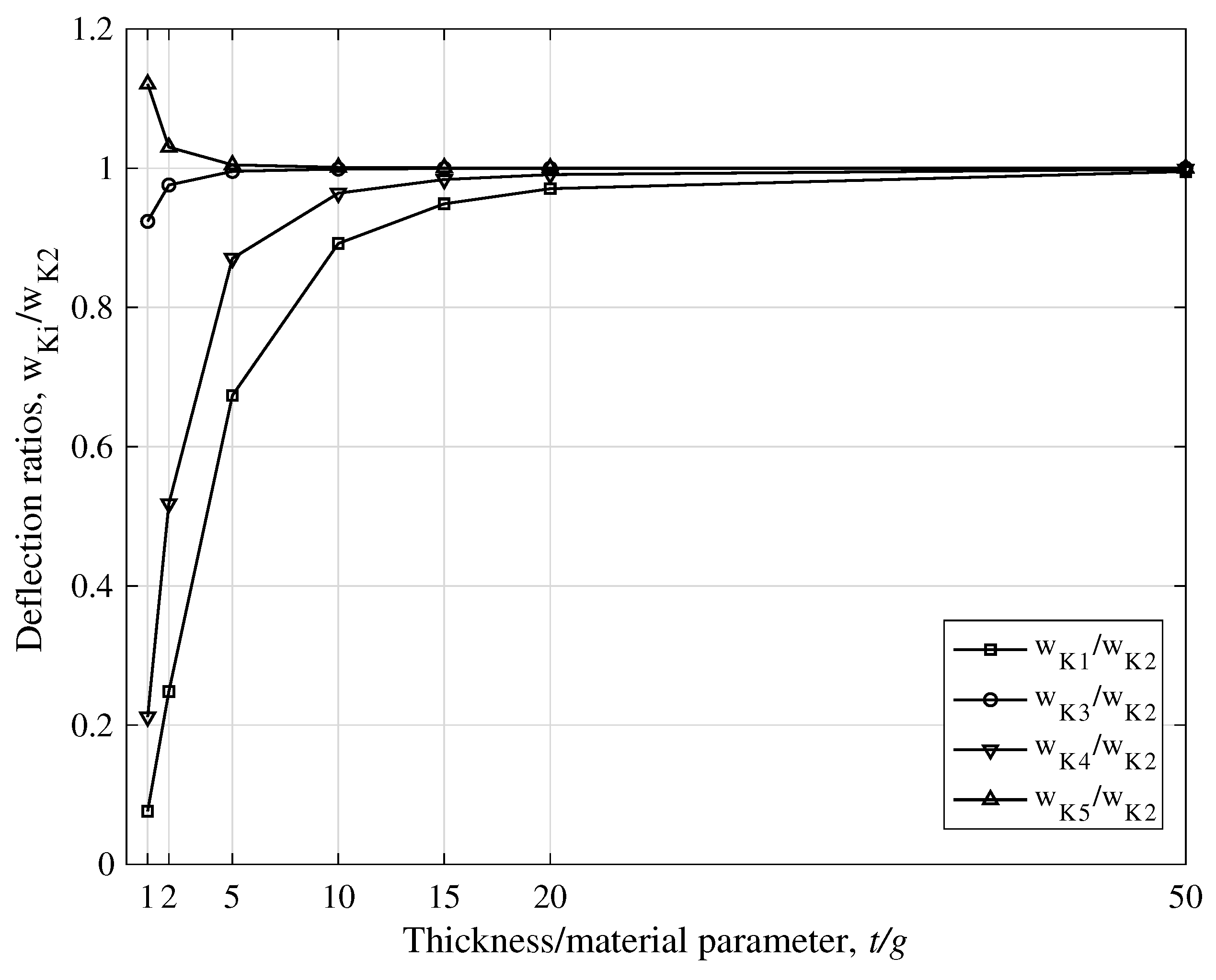
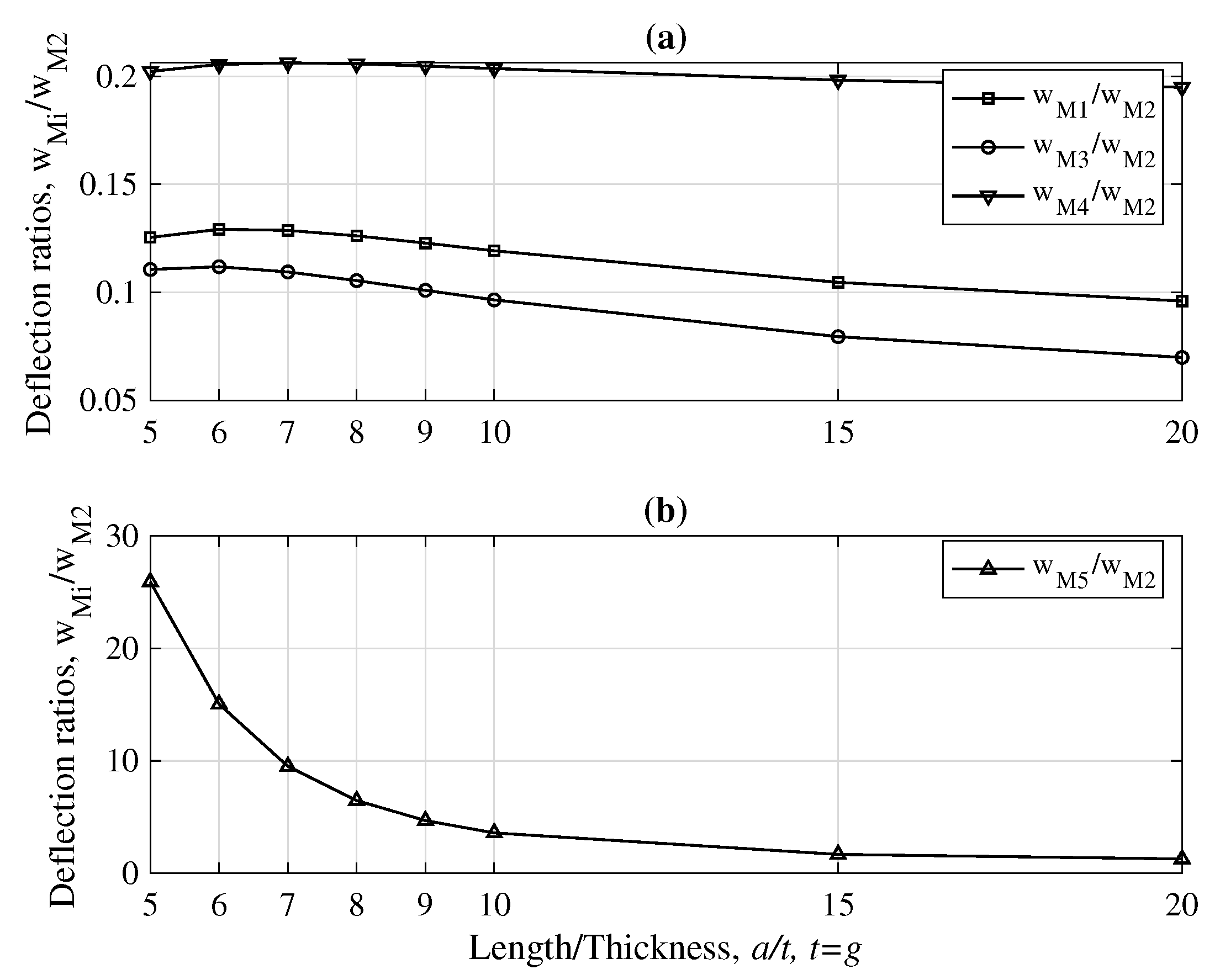
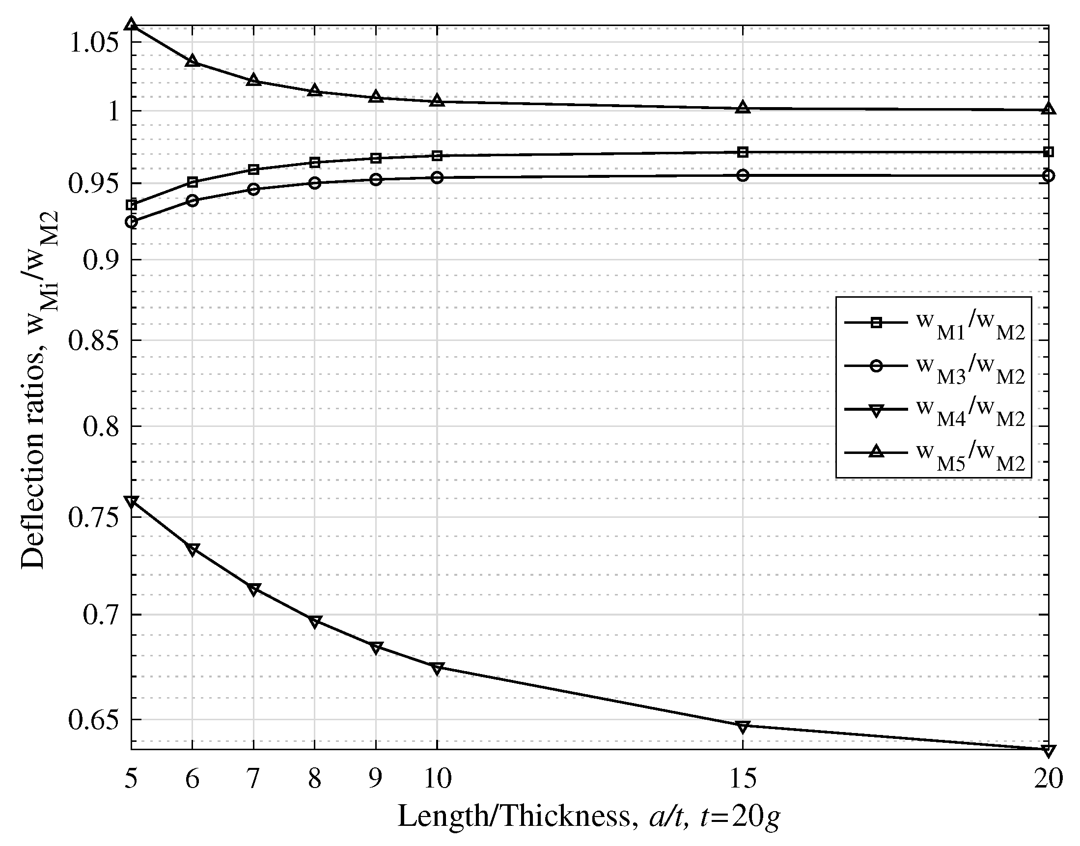
- For plate thickness t is at the micron-scale (small ratio ), models M1, M3 and M4 are stiffer than the classical model M2, while the non-local model M5 is softer than M2. The strain gradient effect is significant both for thick and thin plates, Figure 5, Figure 6, Figure 9 and 10. The same is true for their Kirchhoff counterparts; K1, K3 and K4 are stiffer than K2, while K5 is softer than K2, Figure 7 and Figure 11.
- For larger values of the ratio , models M1, M3 and M5 converge to the classical model M2 for increasing , i.e., for thinner plates. The effect of strain gradient is not completely diminished for thick plates. Additionally, M1 converges to K2 for increasing .
9.2. Conclusions for Free Vibration Response of Micro-Plates
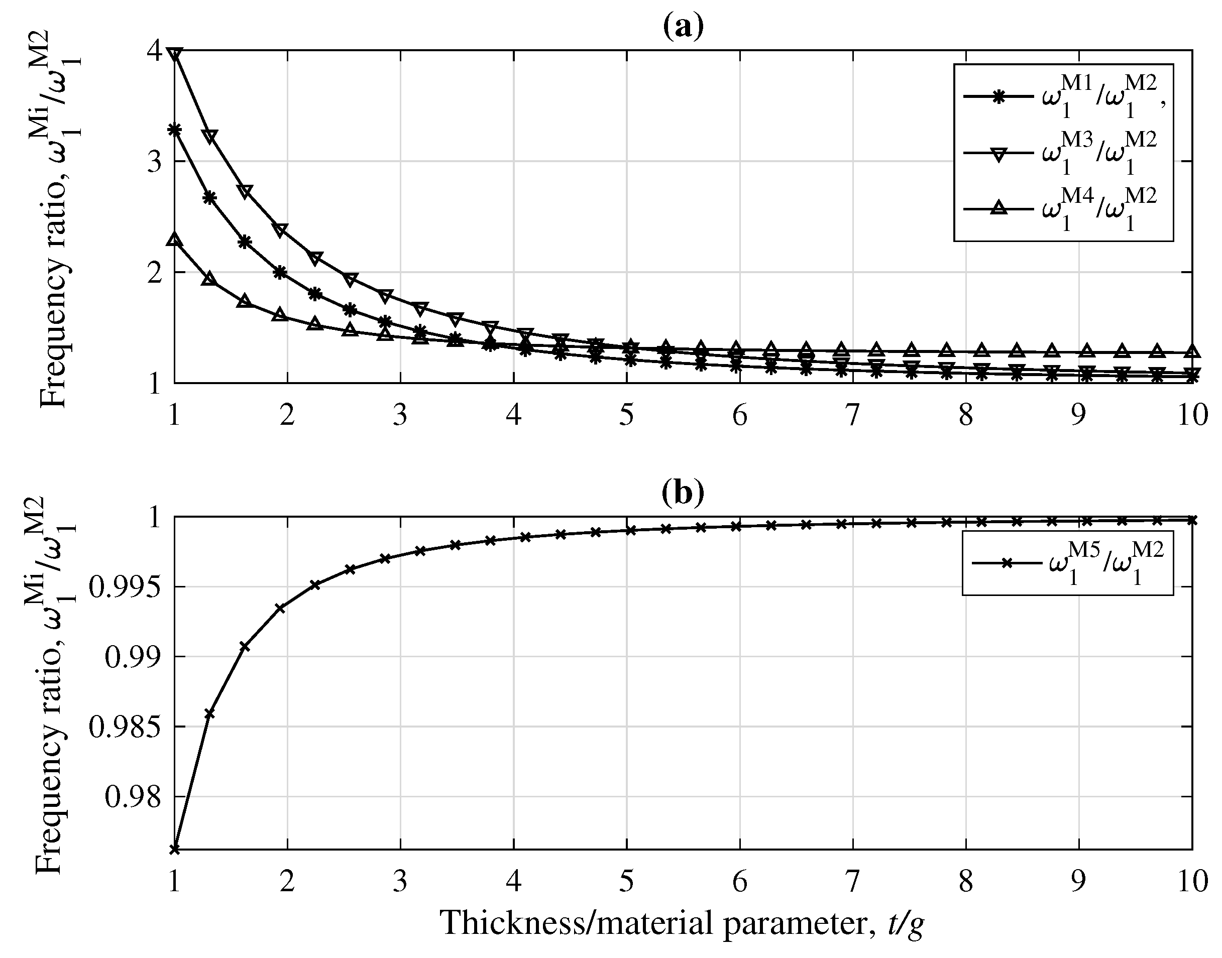
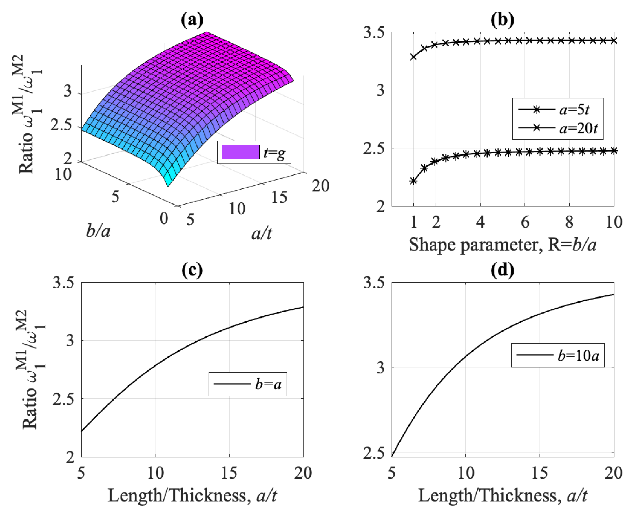
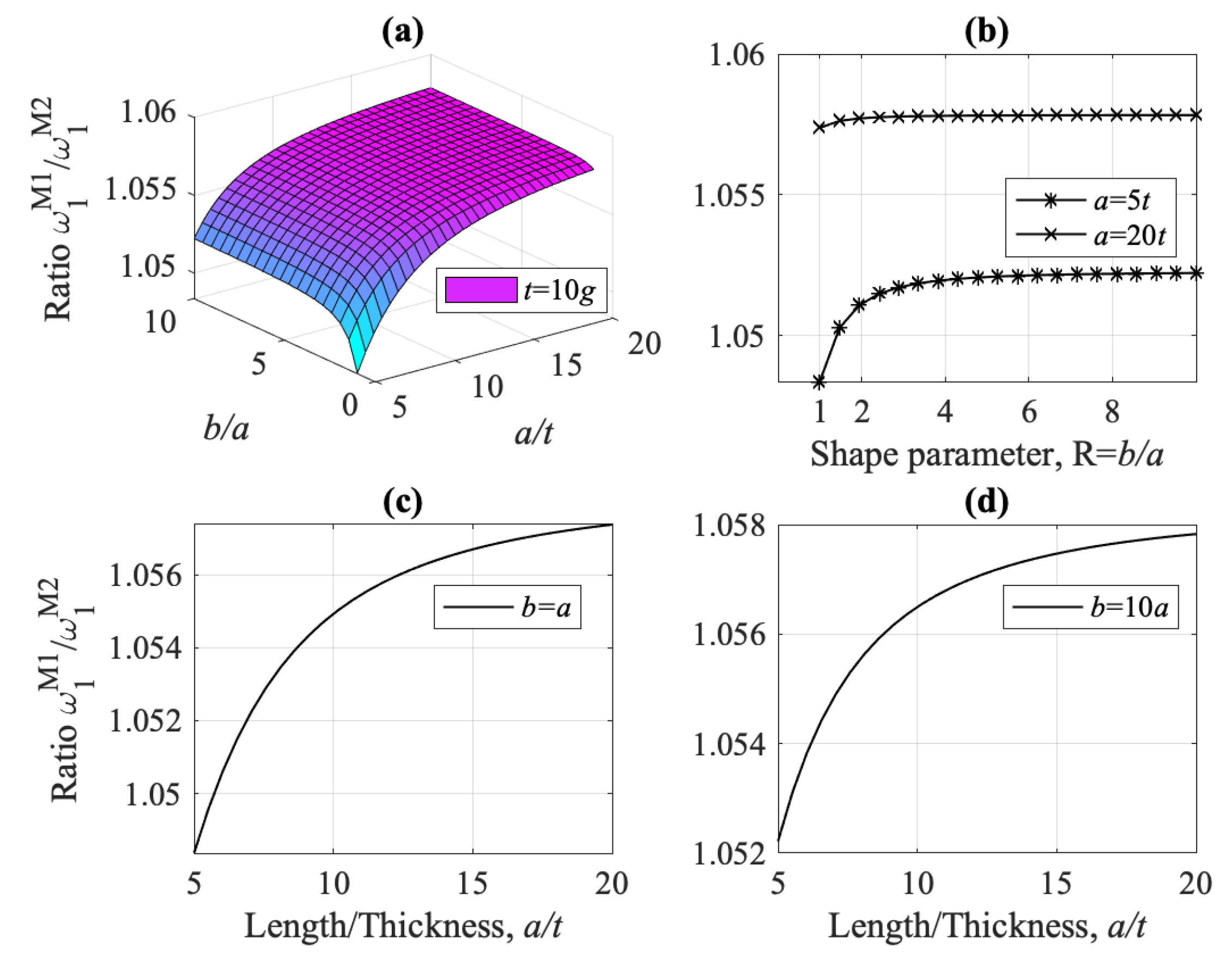
- The flexural fundamental frequency for model M1 is always higher than that of model M2, for every value of the ratios , and , i.e., for thick, thin, square and non-square plates, (see Figure 13, Figure 15, Figure 18 and Figure 19). Shear-thickness frequencies and are, respectively, always lower than those of model M2, for every value of the ratios , and (see Figure 22 and Figure 23).
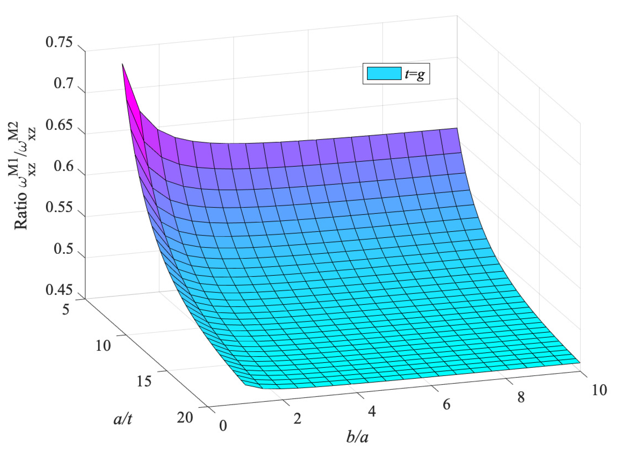
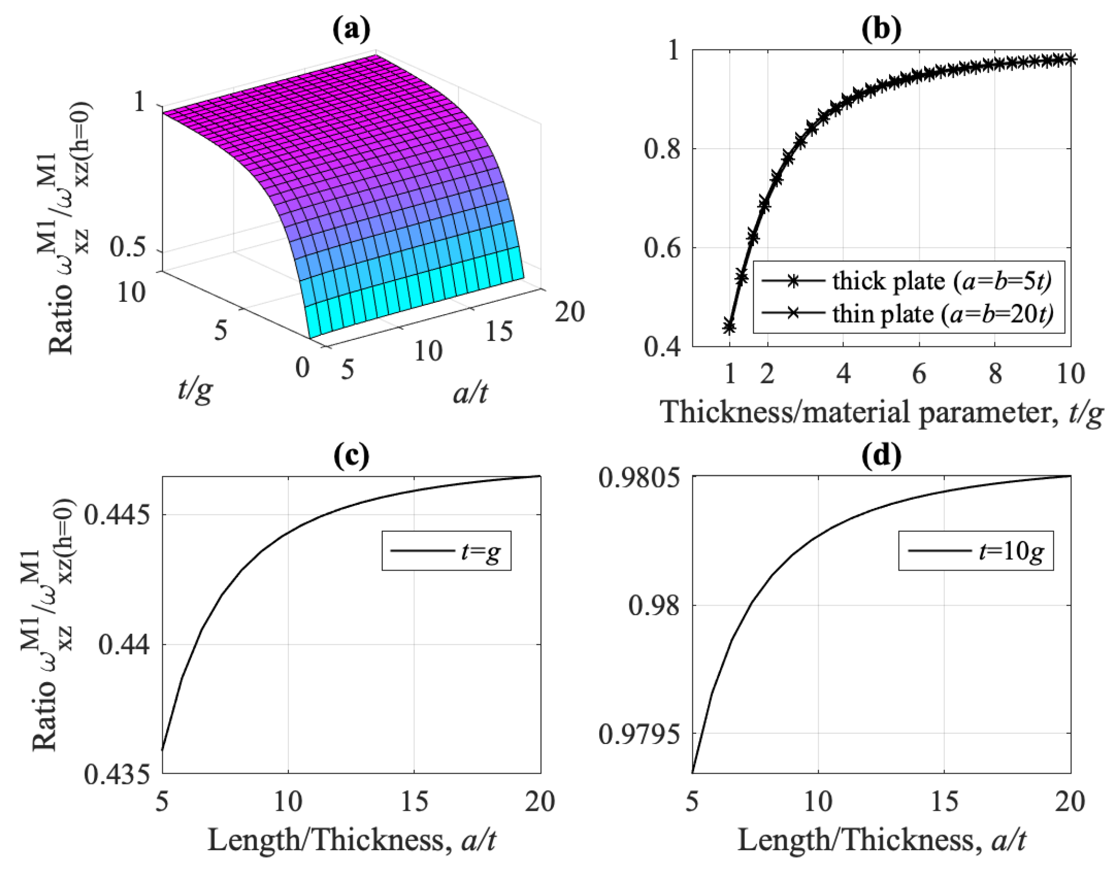
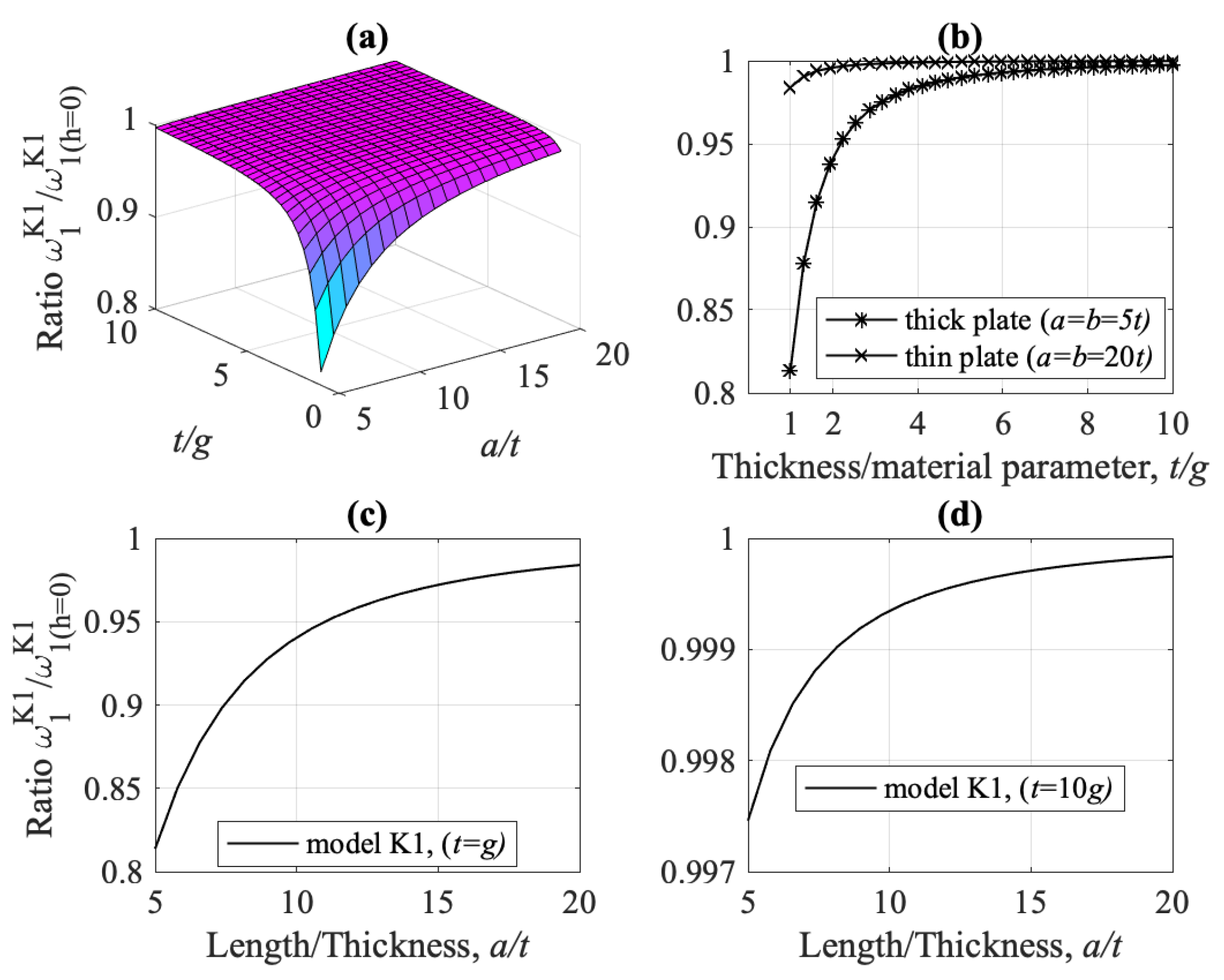
- The strain gradient effect g is mostly significant when plate thickness is at the micron-scale, i.e., for small ratio , both for thick and thin plates, and results in higher values for and lower values for (as compared to model M2). For increasing ratios , frequencies and converge to their classical counterparts, (see Figure 15a and Figure 22, respectively).
- Micro-inertia effect is also significant for the shear-thickness frequency , primarily when the plate thickness is at the micron scale (small ratio ). At any range of the ratio , the frequency is not greatly affected by the ratio , Figure 24.
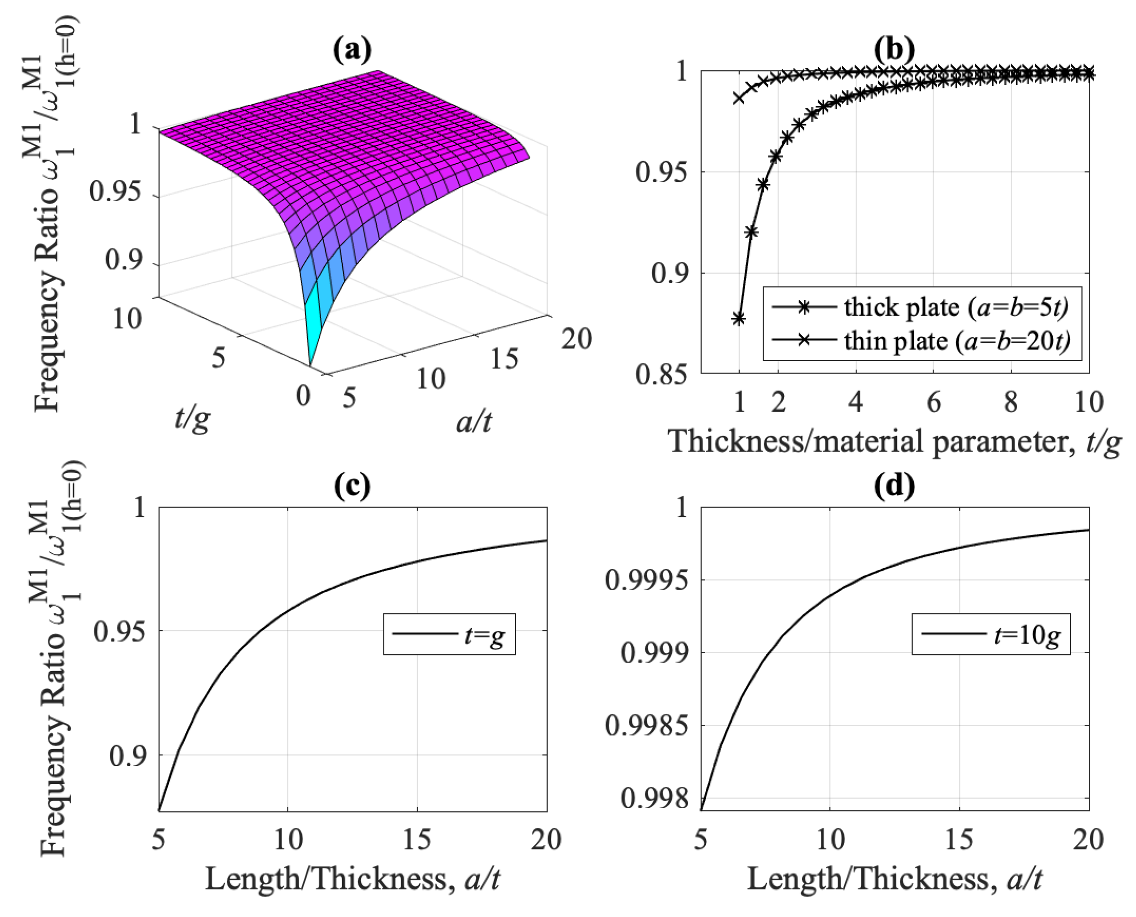
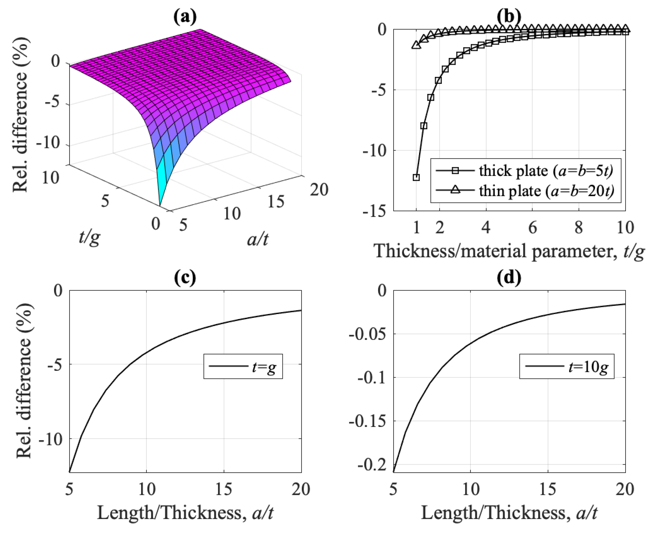
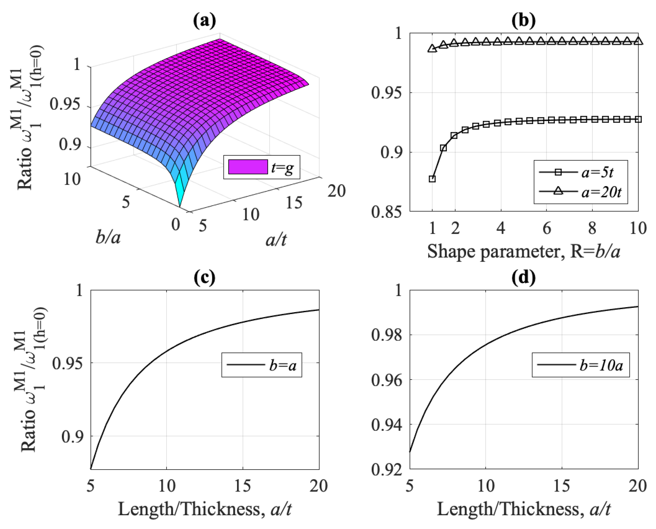
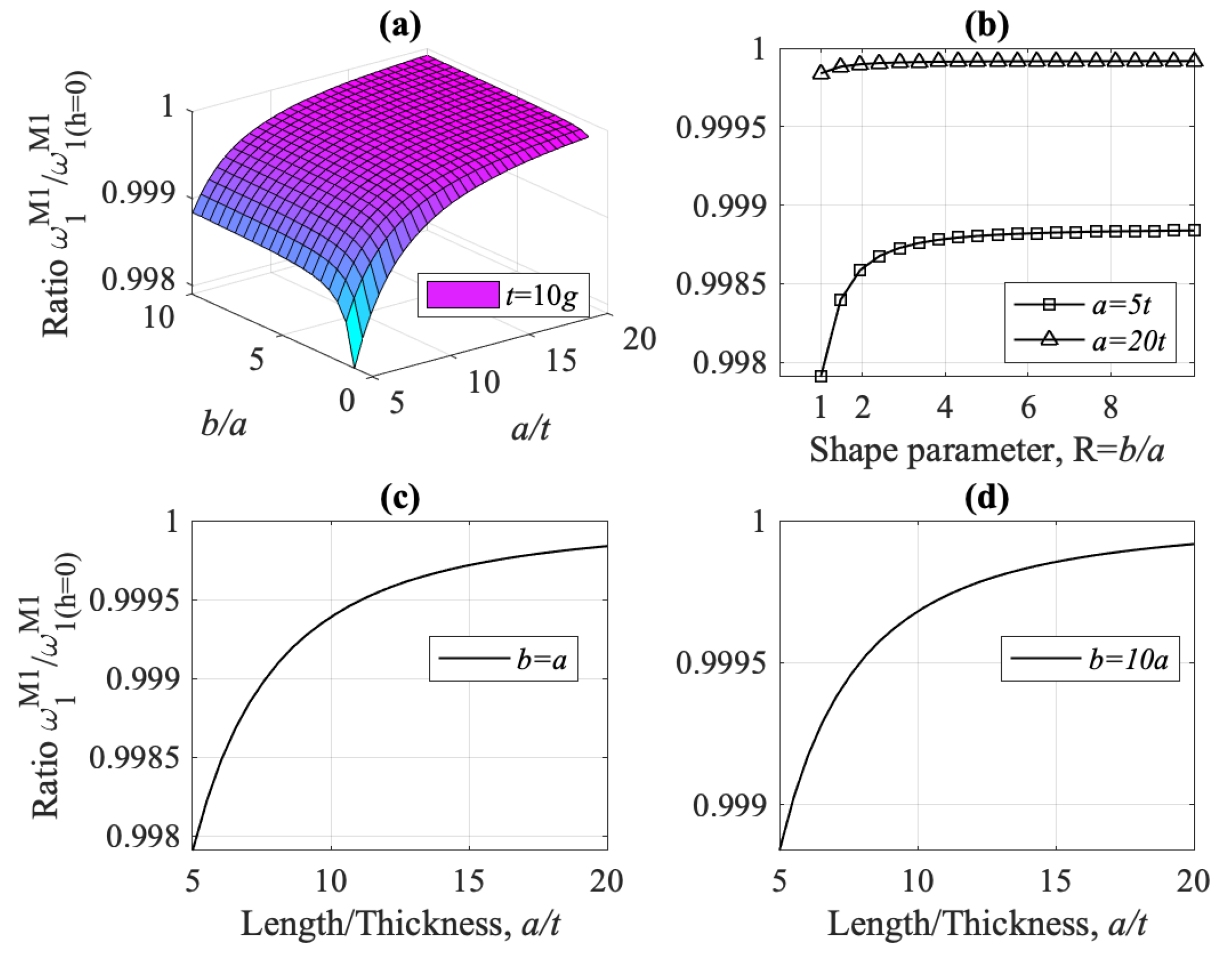
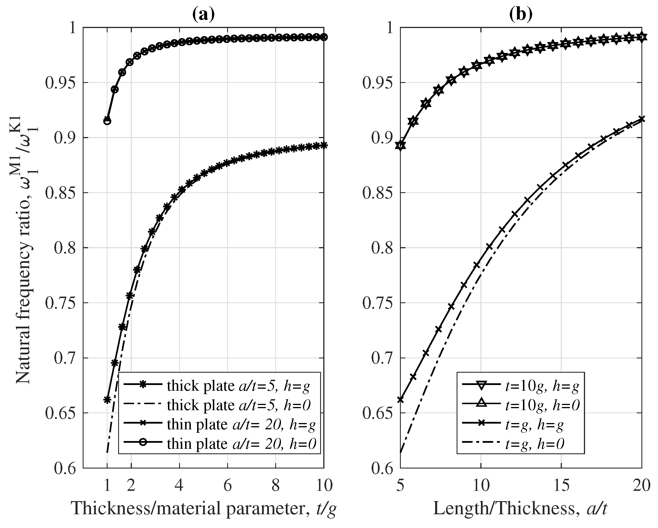
- Considering models M1 and K1, and Figure 27, the combined influence of the shear effect (characteristic of Mindlin–Reissner plates) and the micro-inertia effect, h, on the fundamental frequency was investigated. Model M1 predicts always a smaller frequency than K1. For thick plates, where the shear stresses cannot be ignored, the two models differ significantly, especially for lower values of the ratio . The micro-inertial effect, h, contributes to the difference mostly for thick plates and for lower values of the ratio . For thin plates, the micro-inertial term does not add to the difference in predicted by the two gradient models M1 and K1. For thin plates (increasing ) and when the plate thickness is much larger than the strain gradient parameter g, the two models give similar predictions for .
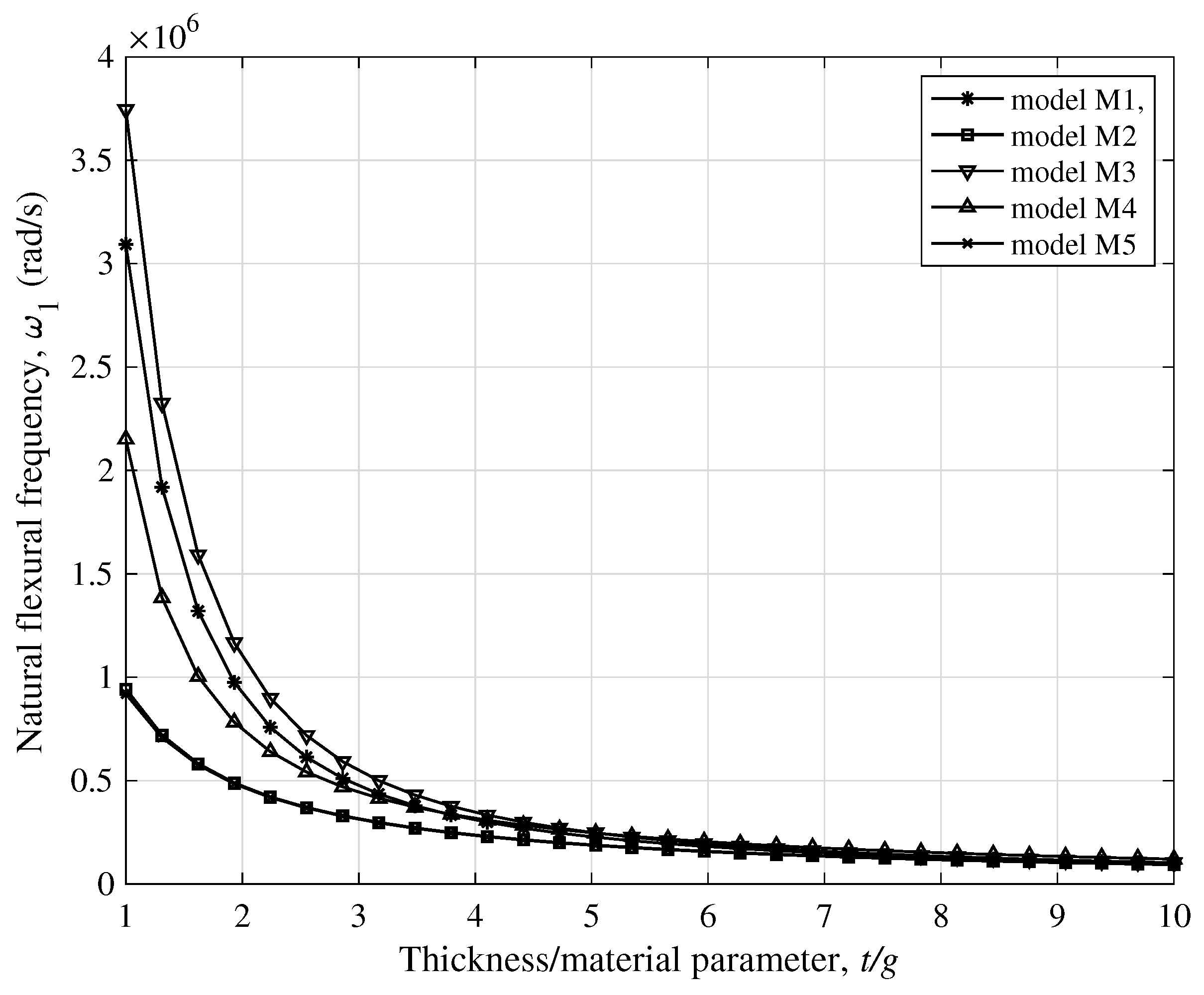
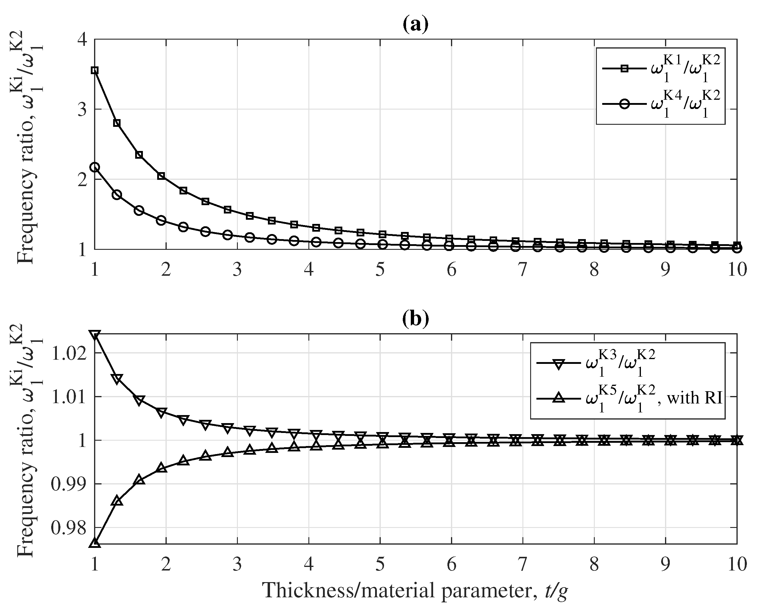
- For plate thickness t is at the micron-scale (small ratio ), models M1, M3, and M4 overestimate the fundamental frequency , as compared to the classical model M2, while model M5 underestimates it, Figure 13. Except model M4, all other models converge to M2 for increasing .
Author Contributions
Funding
Institutional Review Board Statement
Informed Consent Statement
Data Availability Statement
Conflicts of Interest
Appendix A
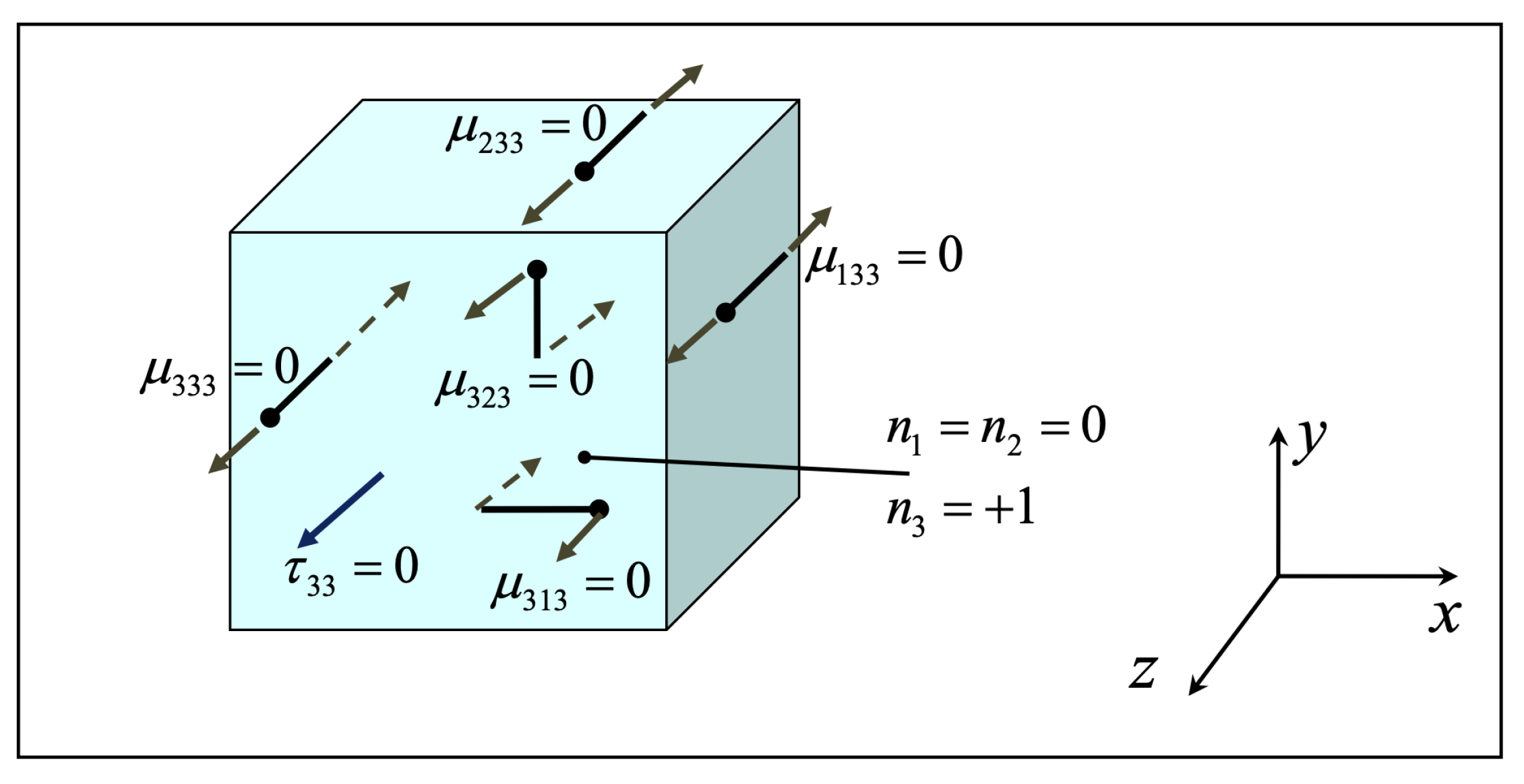
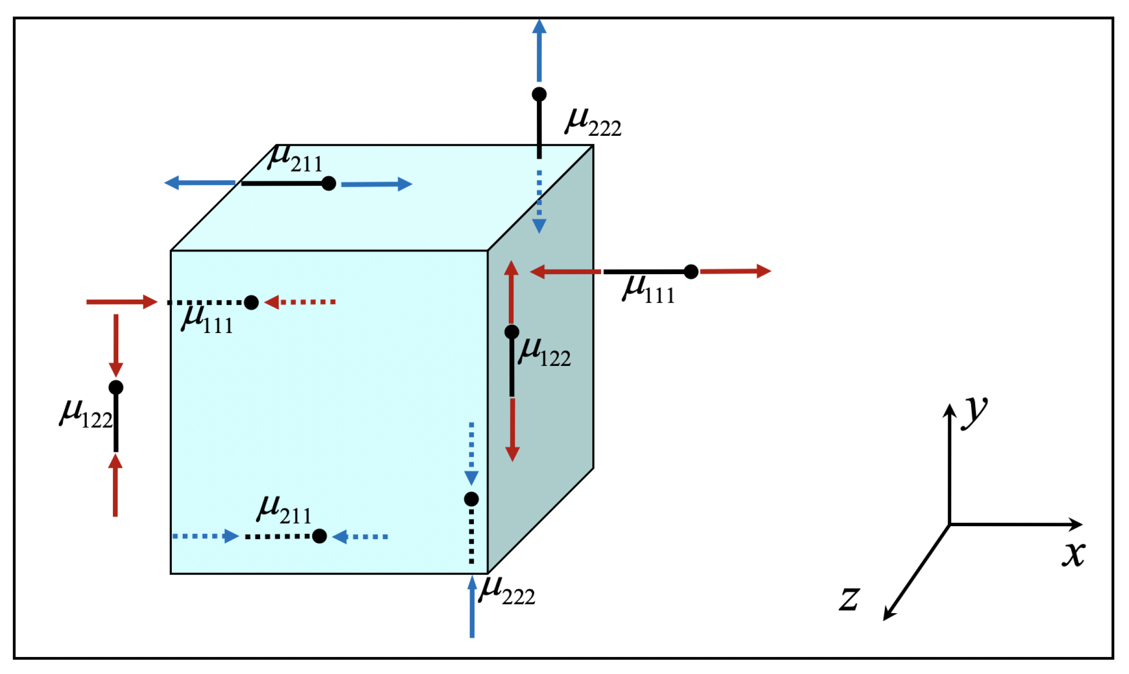
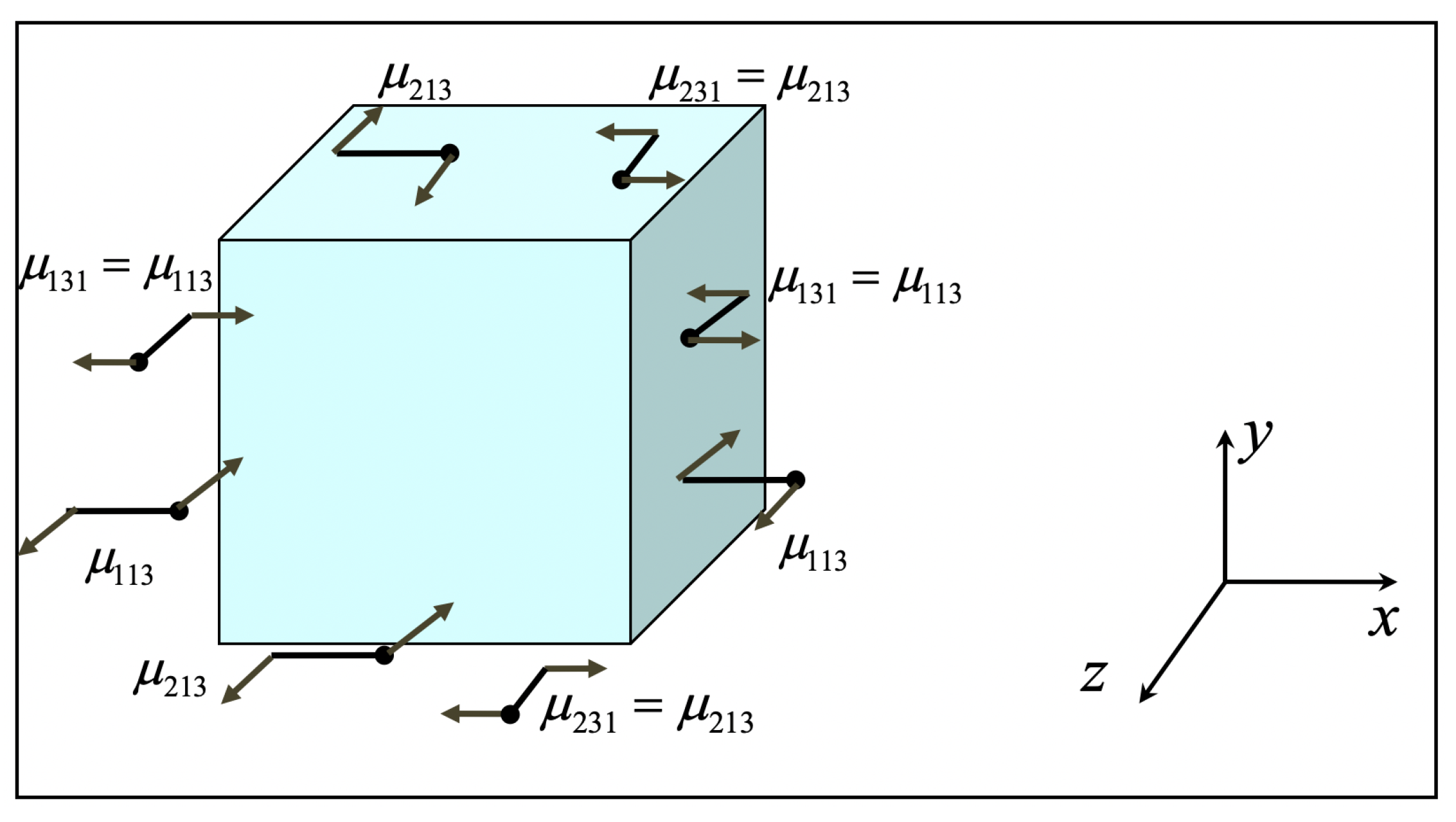
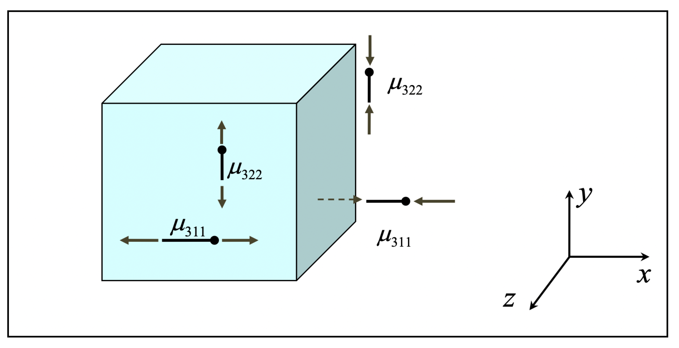
- i denotes the normal to the face on which the double stress acts. For example, acts on the faces (planes) that are normal to the x-axis (1-axis)
- j, direction of the double stress arm. For example, the arm of is along the y-axis (2-axis). The side of the arm which is towards the positive direction of the respective axis is termed as positive arm-side (is marked by a ball-point).
- k, for positive double stress, acting on a positive face, the force on the ball-point (positive arm-side) is towards the positive k-axis (and the other force in the opposite direction).
- For positive double stress, acting on a negative face, the force on the ball-point (positive arm-side) is towards the negative k-axis (and the other force in the opposite direction).
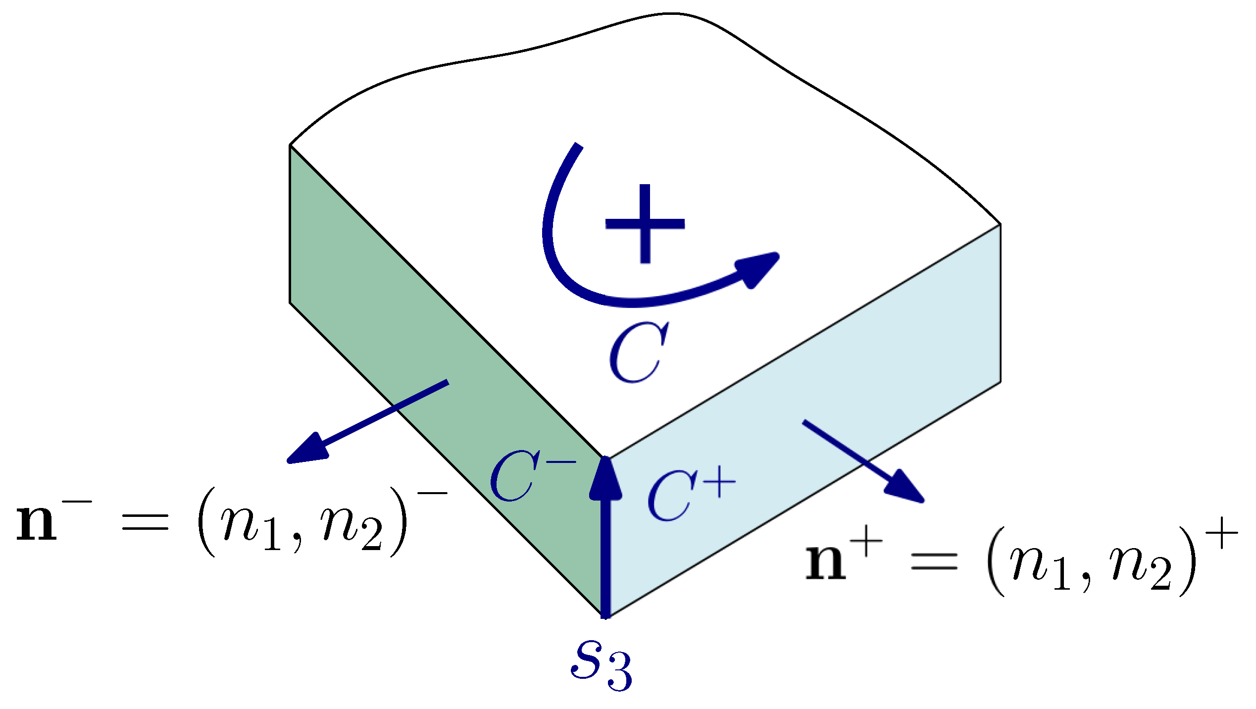
- Positive face: the one which has outer normal towards the positive direction of an axis (1, 2 or 3)
- Negative face: the one which has outer normal towards the negative direction of an axis (1, 2 or 3)
- Note that, at each face of the elementary volume, the total (resultant) moment of the double stresses acting on that face is zero. In other words, the double stress system in strain gradient elasticity is in self-equilibrium at each face.


References
- Senturia, S. Microsystem Design; Kluwer Academic Publishers: Boston, MA, USA, 2001. [Google Scholar]
- Reddy, J. Nonlocal nonlinear formulations for bending of classical and shear deformation theories of beams and plates. Int. J. Eng. Sci. 2010, 48, 1507–1518. [Google Scholar] [CrossRef]
- Zhang, H.; Sun, C. Nanoplate model for platelike nanomaterials. AIAA J. 2004, 42, 2002–2009. [Google Scholar] [CrossRef]
- Giannakopoulos, A.; Stamoulis, K. Structural analysis of gradient elastic components. Int. J. Solids Struct. 2007, 44, 3440–3451. [Google Scholar] [CrossRef][Green Version]
- Mirjavadi, S.S.; Afshari, B.M.; Barati, M.R.; Hamouda, A. Transient response of porous FG nanoplates subjected to various pulse loads based on nonlocal stress-strain gradient theory. Eur. J. Mech. A/Solids 2019, 74, 210–220. [Google Scholar] [CrossRef]
- Ebrahimi, F.; Barati, M.R.; Dabbagh, A. A nonlocal strain gradient theory for wave propagation analysis in temperature-dependent inhomogeneous nanoplates. Int. J. Eng. Sci. 2016, 107, 169–182. [Google Scholar] [CrossRef]
- Fleck, N.; Muller, G.; Ashby, M.; Hutchinson, J. Strain gradient plasticity: Theory and experiment. Acta Metal. Mater. 1994, 42, 475–487. [Google Scholar] [CrossRef]
- Lam, D.; Yang, F.; Chong, A.; Wang, J.; Tong, P. Experiments and theory in strain gradient elasticity. J. Mech. Phys. Solids 2003, 51, 1477–1508. [Google Scholar] [CrossRef]
- MacFarland, A.; Colton, J. Role of material microstructure in plate stiffness with relevance to microcantilever sensors. J. Micromech. Microeng. 2005, 15, 1060–1067. [Google Scholar] [CrossRef]
- Nix, W.; Gao, H. Indentation size effects in crystalline materials: A law for strain gradient plasticity. J. Mech. Phys. Solids 1998, 46, 411–425. [Google Scholar] [CrossRef]
- Markolefas, S.; Papathanasiou, T.; Georgantzinos, S. p-Extension of C0 continuous mixed finite elements for plane strain gradient elasticity. Arch. Mech. 2019, 71, 567–593. [Google Scholar]
- Eringen, C.A.; Edelen, B.D. On nonlocal elasticity. Int. J. Eng. Sci. 1972, 10, 233–248. [Google Scholar] [CrossRef]
- Eringen, A. Theory of nonlocal elasticity and some applications. Res. Mech. 1987, 21, 313–342. [Google Scholar]
- Eringen, A. Nonlocal Continuum Field Theories; Springer: New York, NY, USA, 2002. [Google Scholar]
- Toupin, R. Elastic Materials with Couple-Stresses. Arch. Ration. Mech. Anal. 1962, 11, 385–414. [Google Scholar] [CrossRef]
- Eringen, A. Nonlocal polar elastic continua. Int. J. Eng. Sci. 1972, 10, 1–16. [Google Scholar] [CrossRef]
- Eringen, A. Microcontinuum Field Theories; Springer: New York, NY, USA, 1999; Volume I. [Google Scholar]
- Mindlin, R. Micro-structure in linear elasticity. Arch. Ration. Mech. Anal. 1964, 16, 51–78. [Google Scholar] [CrossRef]
- Mindlin, R. Second gradient of strain and surface-tension in linear Elasticity. Int. J. Solids Struct. 1965, 1, 417–438. [Google Scholar] [CrossRef]
- Mindlin, R.; Eshel, N. On first-gradient theories in linear elasticity. Int. J. Solids Struct. 1968, 4, 109–124. [Google Scholar] [CrossRef]
- Askes, H.; Aifantis, E.C. Gradient elasticity in statics and dynamics: An overview of formulations, length scale identification procedures, finite element implementations and new results. Int. J. Solids Struct. 2011, 48, 1962–1990. [Google Scholar] [CrossRef]
- Amanatidou, E.; Aravas, N. Mixed finite element formulations of strain–gradient elasticity problems. Comput. Methods Appl. Mech. Eng. 2002, 191, 1723–1751. [Google Scholar] [CrossRef]
- Balobanov, V.; Kiendl, J.; Khakalo, S.; Niiranen, J. Kirchhoff–Love shells within strain gradient elasticity: Weak and strong formulations and an H3-conforming isogeometric implementation. Comput. Methods Appl. Mech. Eng. 2019, 344, 837–857. [Google Scholar] [CrossRef]
- Charalambopoulos, A.; Polyzos, D. Plane strain gradient elastic rectangle in tension. Arch. Appl. Mech. 2015, 85, 1421–1438. [Google Scholar] [CrossRef]
- Gavardinas, I.; Giannakopoulos, A.; Zisis, T. A von Karman plate analogue for solving anti-plane problems in couple stress and dipolar gradient elasticity. Int. J. Solids Struct. 2018, 148–149, 169–180. [Google Scholar] [CrossRef]
- Georgiadis, H. The mode III crack problem in microstructured solids governed by dipolar gradient elasticity: Static and dynamic analysis. J. Appl. Mech. 2003, 70, 517–530. [Google Scholar] [CrossRef]
- Gourgiotis, P.; Zisis, T.; Georgiadis, H. On concentrated surface loads and Green’s functions in the Toupin–Mindlin theory of strain-gradient elasticity. Int. J. Solids Struct. 2018, 130–131, 153–171. [Google Scholar] [CrossRef]
- Gourgiotis, P.; Georgiadis, H. Plane-strain crack problems in microstructured solids governed by dipolar gradient elasticity. J. Mech. Phys. Solids 2009, 57, 1898–1920. [Google Scholar] [CrossRef]
- Markolefas, S.; Tsouvalas, D.; Tsamasphyros, G. Some C0 continuous mixed formulations for general dipolar linear gradient elasticity boundary value problems and the associated energy theorems. Int. J. Solids Struct. 2008, 45, 3255–3281. [Google Scholar] [CrossRef][Green Version]
- Lu, L.; Guo, X.; Zhao, J. A unified size-dependent plate model based on nonlocal strain gradient theory including surface effects. Appl. Math. Model. 2019, 68, 583–602. [Google Scholar] [CrossRef]
- Niiranen, J.; Kiendl, J.; Niemi, A.; Reali, A. Isogeometric analysis for sixth-order boundary value problems of gradient-elastic Kirchhoff plates. Comput. Methods Appl. Mech. Eng. 2017, 316, 328–348. [Google Scholar] [CrossRef]
- Niiranen, J.; Niemi, A.H. Variational formulations and general boundary conditions for sixth-order boundary value problems of gradient-elastic Kirchhoff plates. Eur. J. Mech. A/Solids 2017, 61, 164–179. [Google Scholar] [CrossRef]
- Polyzos, D.; Huber, G.; Mylonakis, G.; Triantafyllidis, T.; Papargyri-Beskou, S.; Beskos, D. Torsional vibrations of a column of fine-grained material: A gradient elastic approach. J. Mech. Phys. Solids 2015, 76, 338–358. [Google Scholar] [CrossRef]
- Torabi, J.; RezaAnsari, M. A C1 continuous hexahedral element for nonlinear vibration analysis of nano-plates with circular cutout based on 3D strain gradient theory. Compos. Struct. 2018, 205, 69–85. [Google Scholar] [CrossRef]
- Lu, P.; Zhang, P.; Lee, H.; Wang, C.; Reddy, J. Non-local elastic plate theories. Proc. R. Soc. A 2007, 463, 3225–3240. [Google Scholar] [CrossRef]
- Eringen, A. On differential equations of nonlocal elasticity and solutions of screw dislocation and surface waves. J. Appl. Phys. 1983, 54, 4703–4710. [Google Scholar] [CrossRef]
- Ma, H.; Gao, X.L.; Reddy, J. A non-classical Mindlin plate model on a modified couple stress theory. Acta Mech. 2011, 220, 217–235. [Google Scholar] [CrossRef]
- Tsiatas, G. A new Kirchhoff plate model based on a modified couple stress theory. Int. J. Solids Struct. 2009, 46, 2757–2764. [Google Scholar] [CrossRef]
- Yang, F.; Chong, A.; Lam, D.; Tong, P. Couple stress based strain gradient theory for elasticity. Int. J. Solids Struct. 2002, 39, 2731–2743. [Google Scholar] [CrossRef]
- Lazopoulos, K. On bending of strain gradient micro-plate. Mech. Res. Commun. 2009, 36, 777–783. [Google Scholar] [CrossRef]
- Papargyri-Beskou, S.; Beskos, D. Static, stability and dynamic analysis of gradient elastic flexural Kirchhoff plates. Arch. Appl. Mech. 2008, 78, 625–635. [Google Scholar] [CrossRef]
- Papargyri-Beskou, S.; Giannakopoulos, A.; Beskos, D. Variational analysis of gradient elastic flexural plates under static loading. Int. J. Solids Struct. 2010, 47, 2755–2766. [Google Scholar] [CrossRef]
- Ramezani, S. A shear deformation micro-plate on the most general form of strain gradient elasticity. Int. J. Mech. Sci. 2012, 57, 34–42. [Google Scholar] [CrossRef]
- Filopoulos, S.; Papathanasiou, T.; Markolefas, S.; Tsamasphyros, G. Dynamic finite element analysis of a gradient elastic bar with micro-inertia. Comput. Mech. 2010, 45, 311–319. [Google Scholar] [CrossRef]
- Fafalis, D.; Filopoulos, S.; Tsamasphyros, G. On the capability of generalized continuum theories to capture dispersion characteristics at the atomic scale. Eur. J. Mech. A/Solids 2012, 36, 25–37. [Google Scholar] [CrossRef]
- Bleustein, J. A note on the boundary conditions of Toupin’s strain-gradient theory. Int. J. Solids Struct. 1967, 3, 1053–1057. [Google Scholar] [CrossRef]
- Hughes, T.J.R. The Finite Element Method: Linear Static and Dynamic Finite Element Analysis; Dover Publications, Inc.: Minelola, NY, USA, 2000. [Google Scholar]
- Mindlin, R.; Deresiewicz, H. Thickness-shear and flexural vibrations of rectangular crystal plates. J. Appl. Phys. 1955, 26, 1435–1442. [Google Scholar] [CrossRef]
- Mindlin, R.; Schacknow, A.; Deresiewicz, H. Flexural vibrations of rectangular plates. J. Appl. Mech. 1956, 23, 430–436. [Google Scholar] [CrossRef]
- Reddy, J. Energy Principles and Variational Methods in Applied Mechanics, 2nd ed.; John Wiley & Sons, Inc.: Hoboken, NJ, USA, 2002. [Google Scholar]
- Park, S.; Gao, X. Variational formulation of a modified couple stress theory and its application to a simple shear problem. Z. Angew. Math. Phys. 2008, 59, 904–917. [Google Scholar] [CrossRef]
- Mindlin, R. Influence of rotatory inertia and shear on flexural motions of isotropic, elastic plates. J. Appl. Mech. 1951, 18, 31–38. [Google Scholar] [CrossRef]


| Material Properties and Problem Parameters | Numerical Values |
|---|---|
| Young’s Modulus E (GPa) | 1.44 |
| Poisson ratio | 0.38 |
| Material microscopic parameter g (μm) | 17.6 |
| Micro-inertia parameter h (μm) | 17.6 |
| Material density (kg/m) | 1220.0 |
| Shear correction factor | 5/6 |
| Concentrated load Q (N) | 0.1 |
| Plate thickness t (μm) | Multiple of g, |
| e.g., | |
| Plate dimensions a and b (μm) | Multiple of plate thickness t |
| e.g., |
Publisher’s Note: MDPI stays neutral with regard to jurisdictional claims in published maps and institutional affiliations. |
© 2021 by the authors. Licensee MDPI, Basel, Switzerland. This article is an open access article distributed under the terms and conditions of the Creative Commons Attribution (CC BY) license (https://creativecommons.org/licenses/by/4.0/).
Share and Cite
Markolefas, S.; Fafalis, D. Strain Gradient Theory Based Dynamic Mindlin-Reissner and Kirchhoff Micro-Plates with Microstructural and Micro-Inertial Effects. Dynamics 2021, 1, 49-94. https://doi.org/10.3390/dynamics1010005
Markolefas S, Fafalis D. Strain Gradient Theory Based Dynamic Mindlin-Reissner and Kirchhoff Micro-Plates with Microstructural and Micro-Inertial Effects. Dynamics. 2021; 1(1):49-94. https://doi.org/10.3390/dynamics1010005
Chicago/Turabian StyleMarkolefas, Stylianos, and Dimitrios Fafalis. 2021. "Strain Gradient Theory Based Dynamic Mindlin-Reissner and Kirchhoff Micro-Plates with Microstructural and Micro-Inertial Effects" Dynamics 1, no. 1: 49-94. https://doi.org/10.3390/dynamics1010005
APA StyleMarkolefas, S., & Fafalis, D. (2021). Strain Gradient Theory Based Dynamic Mindlin-Reissner and Kirchhoff Micro-Plates with Microstructural and Micro-Inertial Effects. Dynamics, 1(1), 49-94. https://doi.org/10.3390/dynamics1010005