Reactive Molecular Dynamics in Ionic Liquids: A Review of Simulation Techniques and Applications

Abstract

Ionic liquids exhibit distinctive solvation and reactive properties, making them highly relevant for applications in energy storage, catalysis, and CO₂ capture. However, their complex molecular interactions, including proton transfer and physisorption/chemisorption, necessitate advanced computational efforts to model them at the atomic scale. This review examines key molecular dynamics approaches for simulating ionic liquid reactivity, including quantum-mechanical methods, conventional reactive force fields such as ReaxFF, and fractional force fields employed in PROTEX. The strengths and limitations of each method are assessed within the context of ionic liquid simulations. While quantum-mechanical simulations provide detailed electronic insights, their high computational cost restricts system size and simulation timescales. Reactive force fields enable bond breaking and formation in larger systems but require extensive parameterization. These approaches are well suited for investigating reaction pathways influenced by the local environment, which can also be partially addressed using multiscale simulations. Fractional force fields offer an efficient alternative for simulating significantly larger reactive systems over extended timescales. Instead of resolving individual reaction mechanisms in full detail, they incorporate reaction probabilities to model complex coupled reactions. This approach enables the study of macroscopic properties, such as conductivity and viscosity, as well as proton transport mechanisms like the Grotthuß process—phenomena that remain inaccessible to other computational methods.

1. Introduction

Solvents are often considered secondary players in many chemical reactions [1], primarily contributing solvation energy to the overall free energy of the system. However, their direct interaction with reactants can significantly impact reaction pathways by lowering activation energies or generating electric fields that alter the potential energy surface. Among solvents, ionic liquids (ILs) are a fascinating class of charged, dipolar systems capable of modulating and accelerating various chemical reactions [2,3].

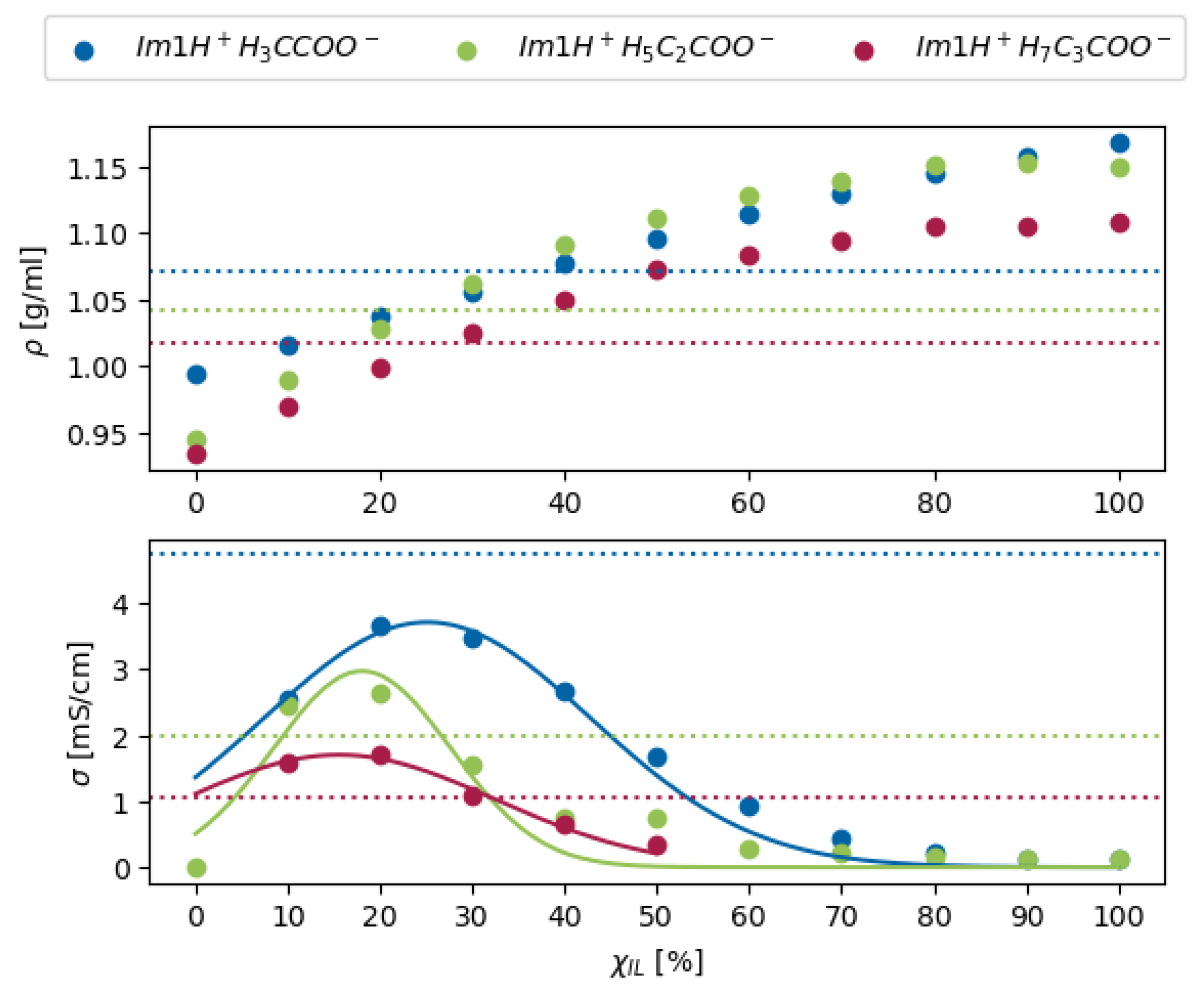
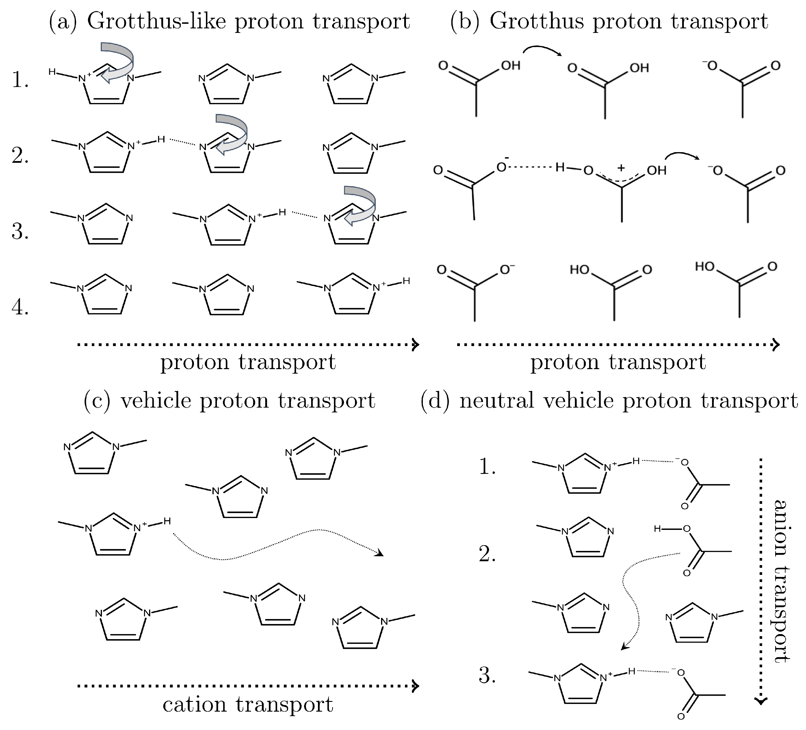
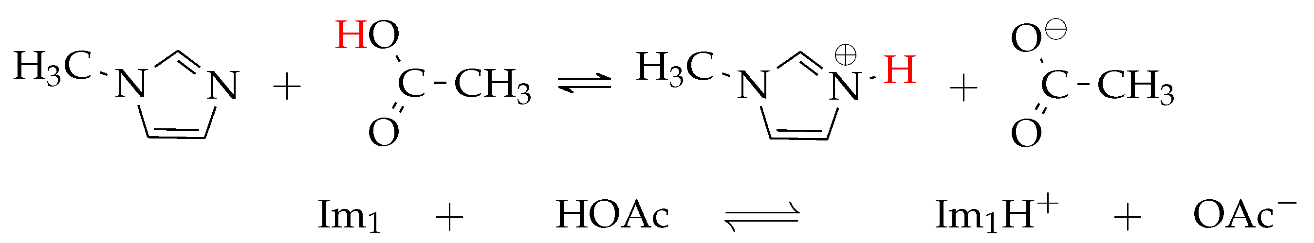
1.1. Proton Transfer Reactions in Ionic Liquids

Protic ILs [4,5,6,7] have garnered significant attention due to their dual functionality as solvents and reactants, particularly in proton transfer reactions exemplified by the equilibrium:

$$\begin{array}{ccc}{\mathrm{HA}}^{+}+ {\mathrm{B}}^{-}& \rightleftharpoons & \mathrm{A}+\mathrm{HB}\end{array}$$

(1)

Their distinctive hydrogen-bonding networks facilitate this dual role [6,8,9] as hydrogen bonds strengthen the interaction with solutes, and a hydrogen bond is a prerequisite for a subsequent proton transfer. The strength of these hydrogen bonds is contingent upon the specific ionic partners and their relative acid-base characteristics. The degree of ionization within a protic IL is quantitatively governed by the $\Delta p{K}_a=p{K}_a\left({\mathrm{HA}}^{+}\right)-p{K}_a\left(\mathrm{HB}\right)$ difference between the acidic cation HA⁺ and the conjugate acid of the base HB [4,5,10]. Differences in $\Delta p{K}_a$ larger than 6 signify complete ionization and distinctive ionic behavior, whereas smaller values result in partial proton transfer [11], leaving a fraction of neutral molecular species [10]. Such partial ionization can compromise IL properties, leading to phase separation or evaporation. Nevertheless, these pseudo-ionic systems still exhibit significant conductivities [6,12,13,14,15,16,17]. Determining the precise composition of protic ILs has proven challenging due to discrepancies among experimental methodologies (NMR [18,19,20,21,22,23], quasi-elastic neutron scattering [22], small-angle X-ray scattering [21,23], Raman [10,24] and IR spectroscopy [23,25,26]). Umebayashi et al. [27,28,29] employed potentiometric titration to assess proton activities in several protic ILs. Unlike other protic ILs, such as ethylammonium nitrate, the 1-methylimidazole/acetic acid system showed no significant jump in the potentiometric titration curve. Based on calorimetric titration, they estimated a negative $p{K}_a$ of −1.4, corresponding to a neutral species content of approximately 66.4%. Using density measurements, Qian et al. [30] and Hou et al. [13] calculated slightly different values, ranging from 62.7 to 68.6%. Subsequent Raman spectroscopic analysis by Umebayashi’s group revised this estimation, suggesting that the content of neutral species could be as high as 99.0% [10]. In stark contrast, Chen et al. [19] reported a neutral species content of merely 7.2%, based on NMR spectroscopy. Despite these discrepancies, there is a consensus that the ionic character of the 1-methylimidazole/acetic acid system is notably low, disqualifying it as a fully ionic liquid.

Despite the predominance of neutral molecules in such systems, they can still exhibit significant ionic conductivities, such as the 4 mS/cm reported for 1-methylimidazole/acetic acid [31]. According to Angell’s classification, based on Walden behavior, such liquids are categorized as good or even superionic conductors [31]. A Grotthuß-like proton conduction mechanism has been proposed to rationalize this high conductivity, wherein protons hop between ionic and neutral species via low-energy barrier transitions [32]. This Grotthuß mechanism, well studied in molecular liquids such as water, enables rapid charge transport without requiring the physical migration of the proton itself. Instead, the proton charge is relayed through the liquid via successive hydrogen-bond reorganization. The extended three-dimensional hydrogen-bond networks required for this mechanism have been observed in protic ILs such as ethylammonium nitrate [8] and are expected in other protic ILs [33,34]. This mechanism provides a significant advantage over the slower vehicle mechanism, where proton transport relies on the diffusion of ions. Although these studies showed that Grotthuß-like transport is a more general mechanism than previously thought, current evidence is still sparse, and the molecular dynamics of proton conduction in protic ILs are not yet fully understood. Developing reliable methodologies for modeling proton transfer dynamics in ILs is essential due to their widespread use as prototypical conductive media in energy storage and conversion devices to design advanced superprotonic systems, but also because their acidic and basic properties inherently influence their interactions with other molecules [35]. Moreover, the proton activity of acids in related systems, such as deep eutectic solvents and other ionic liquids, has been quantified in terms of $p{K}_a$ values but has yet to be explored at the molecular level [36,37]. These studies could provide new insights into designing protic ILs with tailored properties for specific applications.

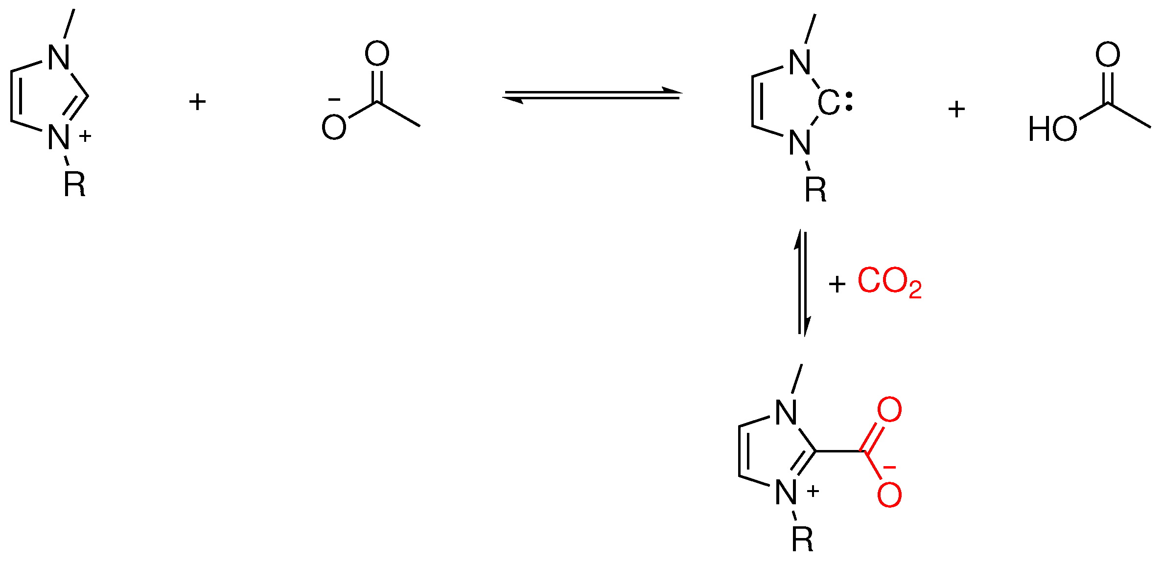
1.2. Chemisorption in Ionic Liquids

Since the early 2000s, ILs have garnered significant attention as potential alternatives to traditional amine-based technologies in CO₂ separation processes [38,39,40]. Their unique properties, such as low volatility, tunable structures, and high thermal stability, make them particularly attractive for CO₂ capture applications. However, subsequent studies [39,40,41,42] have identified several challenges that hinder the practical implementation of ILs in this context. These include difficulties in regenerating ILs after CO₂ capture, increased viscosity upon CO₂ absorption, challenges associated with fluorinated anions, high operational and material costs, and the intricate synthesis processes required for tailored ILs [38,39,40]. These findings underscore the need for further research and innovation to overcome these limitations and establish ILs as a viable alternative to conventional CO₂ capture technologies. Effective CO₂ capture necessitates high CO₂ loading at low pressures [40], which cannot be achieved through physical absorption alone [43]. Chemical absorption, while offering the necessary reactivity, must remain energetically moderate and reversible to enable efficient regeneration of the absorbent. Therefore, optimizing the balance between physical and chemical absorption mechanisms is critical for designing advanced IL-based solutions for CO₂ capture.

ILs with mild acid-base characteristics, particularly those based on imidazolium and phosphonium carboxylates [43,44,45,46,47,48,49,50,51], have demonstrated promise in enabling CO₂ chemisorption through the formation of an imidazolium carbene. As illustrated in Figure 1, the initial chemisorption step involves a proton transfer from 1-alkyl-3-methylimidazolium to acetate, yielding an N-heterocyclic carbene (NHC, also known as an Arduengo carbene [52]) and acetic acid [53]. This equilibrium is primarily dictated by the anion’s $p{K}_a$ or its Kamlet–Taft $\beta$ parameter. However, obtaining and comparing these parameters remains challenging due to inconsistencies in measurement techniques and the influence of the surrounding medium. For example, Daniele et al. [49] demonstrated that while acetate anions ($p{K}_a=4.26$) are highly effective for CO₂ activation, their fluorinated counterpart, CF₃COO⁻ ($p{K}_a=0.23$), is inactive due to its lower basicity. This highlights the importance of fine-tuning the anion’s $p{K}_a$ to enhance CO₂ pre-activation and facilitate subsequent reduction in the presence of an electron donor, such as electrodes or semiconductors. Additionally, the structure of the protonated anion may provide a synergistic effect by serving as a proton source. Upon CO₂ introduction, the equilibrium competes with forming a zwitterionic imidazolium-CO₂ adduct. Stabilized by hydrogen bonding to an adjacent 1-alkyl-3-methylimidazolium cation, this adduct produces a 1:2 (CO₂:IL) stoichiometry. The adduct represents an activated form of CO₂, characterized by a bent geometry and partial electron transfer from the NHC to CO₂, yielding CO₂⁻, a key intermediate in CO₂ (photo)reduction pathways. Notably, the CO₂ pressure influences the $p{K}_a$ of 1-alkyl-3-methylimidazolium, further complicating the dynamic interactions within the IL system. The anion’s ability to complex with any acid formed during the process, effectively acting as an internal buffer, adds a layer of complexity crucial for the practical application of these ILs in CO₂ capture and conversion technologies.

1.3. Demand for Computational Studies

The intricate heterogeneous structure and dynamics of ILs present significant challenges for experimental techniques [33]. Their broad temperature ranges and varying degrees of interaction between the cationic and anionic components result in many possible structural organizations and dynamics, often rendering direct experimental observation impractical. Computational simulations, however, offer a powerful alternative by providing detailed insights at the atomic level [54]. These simulations act as a computational microscope, enabling researchers to explore ions’ arrangement, dynamics, and interactions under various conditions. Under experimentally challenging scenarios, they can predict critical properties like structure, transport, and thermodynamics. Furthermore, simulations facilitate the design and optimization of ILs with tailored properties, offering a cost-effective, predictive approach to developing new materials.

Reactive molecular dynamics simulations [35,55] have proven particularly valuable in studying the microscopic mechanisms by which ILs influence chemical reactions. By capturing the dynamics of bond formation and cleavage in real time, these simulations provide detailed insights into reaction mechanisms, including transient intermediates and transition states that are challenging to identify experimentally. They allow for exploring complex reaction pathways, predicting likely routes, and quantifying competing pathways’ probabilities. This capability extends to non-ideal conditions, such as those in condensed phases, at interfaces, or within biological systems, where experimental studies may be limited. Reactive molecular dynamics also shed light on reaction kinetics, revealing rates and lifetimes of transient species under extreme conditions, such as high pressure, temperature, or strong electric fields. Even without chemical reactivity, accurately modeling ILs remains a formidable challenge [56]. These systems are characterized by high viscosity, strong Coulombic interactions, significant dispersion forces, and numerous possible cation–anion combinations. Experimental results on the composition of (pseudo-) protic ILs are often inconclusive and contradictory. Simulations offer critical insights into these compositions and how such complex media influence reaction pathways, stabilize intermediates, and alter reaction rates. This review focuses on these reactions within ILs while providing an overview of reactive molecular dynamics simulation techniques. Although not all methods discussed have been explicitly applied to ILs, they are included to highlight their potential utility in advancing our understanding of these versatile and complex systems.

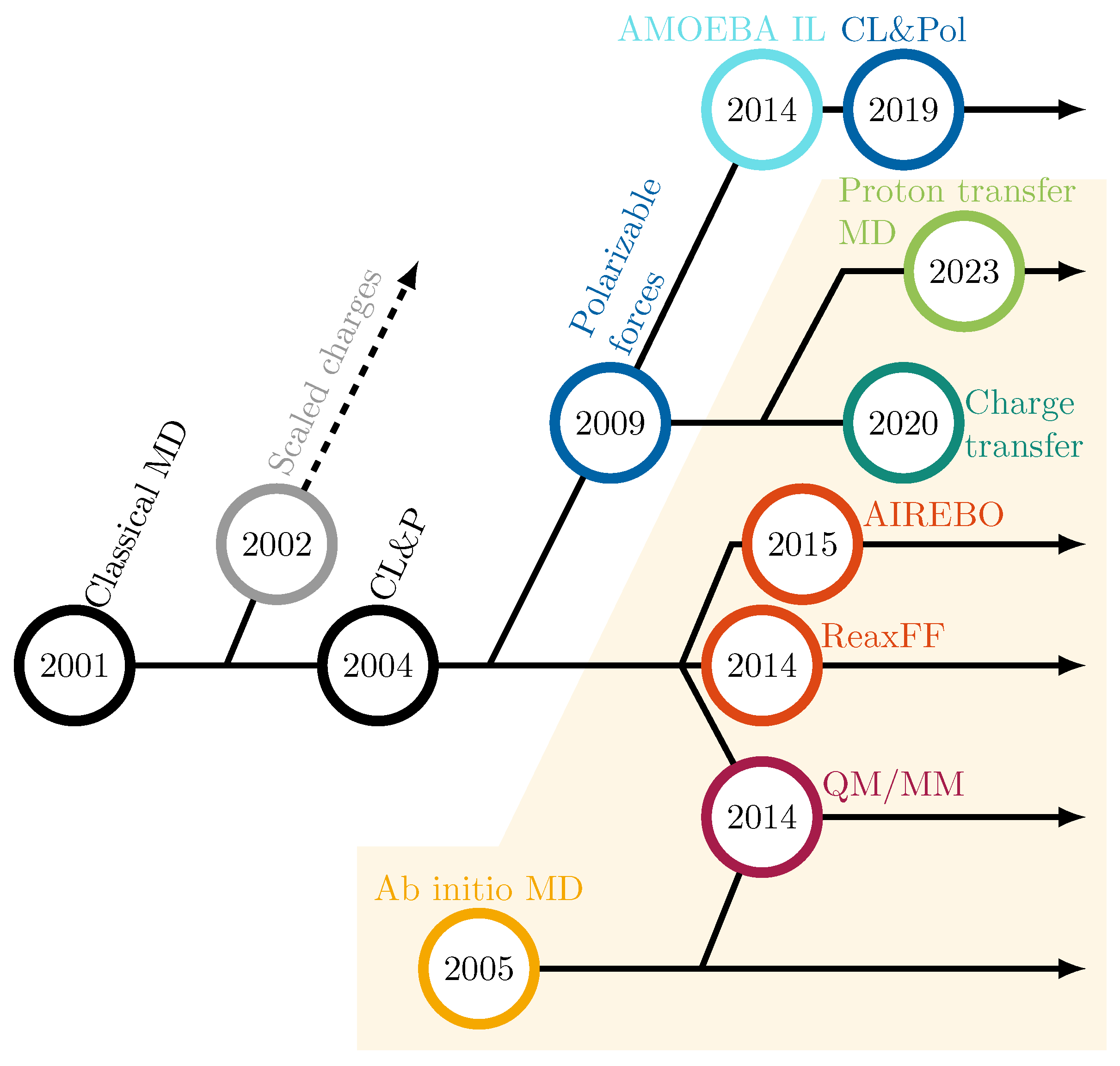
2. Theoretical Investigations

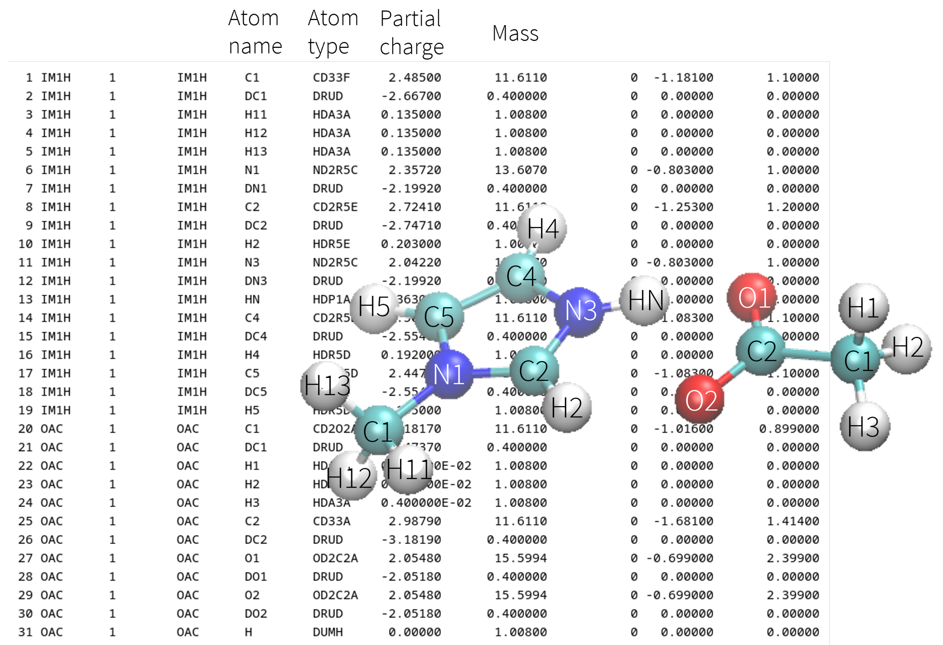
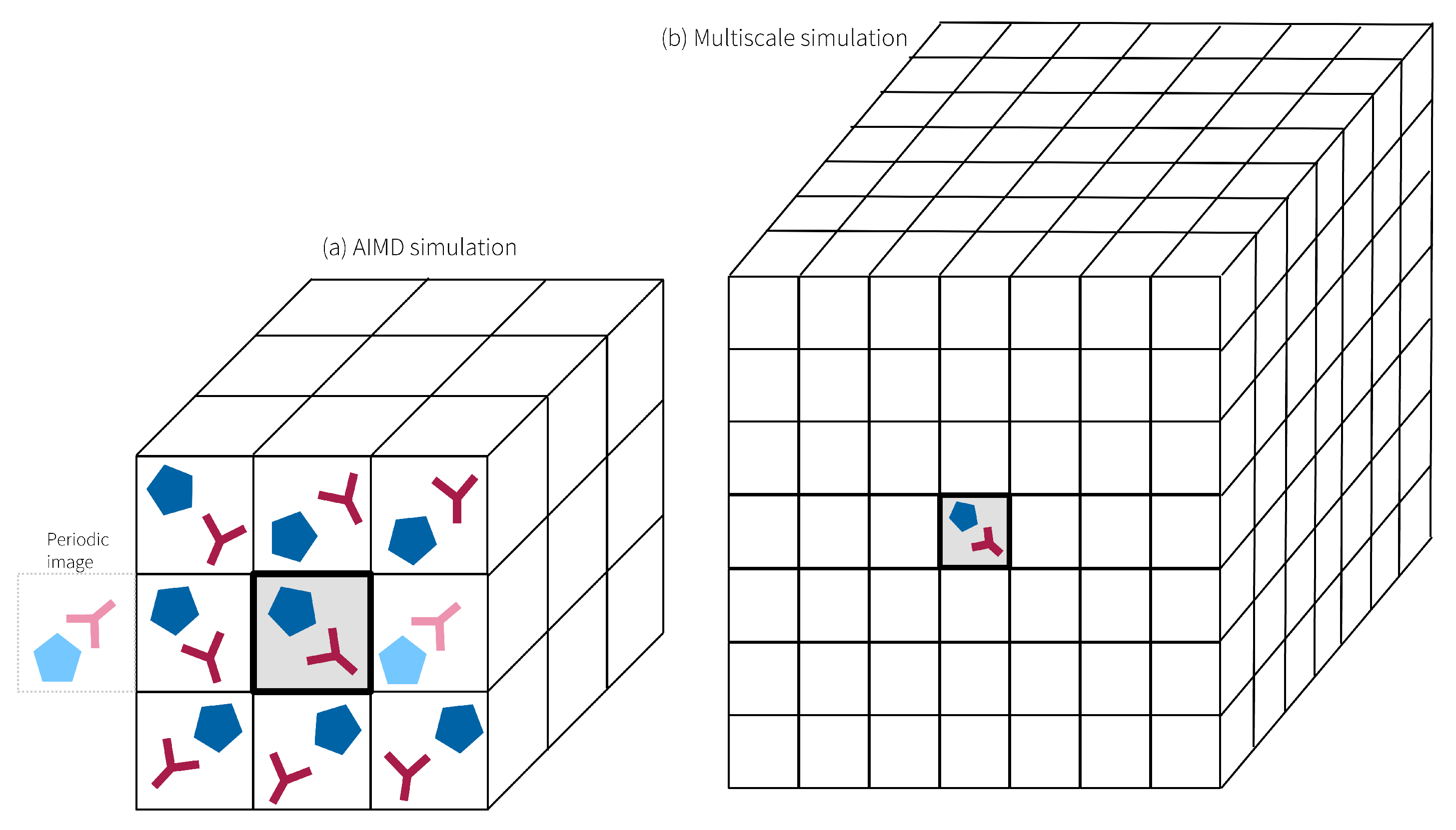
2.1. Fundamentals of Conventional, Fixed-Charge Molecular Dynamics Simulations

A recent comprehensive review [57] on the fundamental methodologies and future perspectives of conventional molecular dynamics (MD) simulations provides an in-depth analysis of clever force field calibration to align with experimental and quantum-mechanical (QM) data. Additionally, it outlines various advanced techniques for efficient sampling of configurational space and the derivation of physicochemical properties through statistical mechanics. Fixed-charge MD simulations are extensively utilized for investigating ILs, offering profound insights into their structural and dynamic properties [56,58,59,60]. They rely on predefined force fields incorporating intramolecular potentials, such as bond stretching $U^{bond}(r_i,r_j)$, angular bending $U^{angle}(r_i,r_j,r_k)$, dihedral and improper torsions $U^{torsions}(r_i,r_j,r_k,r_l)$, as well as intermolecular interactions modeled through Lennard–Jones $U^{LJ}(r_i,r_j)$ and Coulomb potentials $U^{Coulomb}(r_i,r_j)$:

$$\begin{array}{ccc}\hfill U_{FF}& =& {\displaystyle \sum _{ij}^{bonds}{U}^{bond}(r_i,r_j)+\sum _{ijk}^{angles}{U}^{angle}(r_i,r_j,r_k)+\sum _{ijkl}^{torsions}{U}^{torsions}(r_i,r_j,r_k,r_l)}\hfill \\ \hfill & +& {\displaystyle \sum _i\sum _{j>i}{U}^{LJ}(r_i,r_j)+\sum _i\sum _{j>i}{U}^{Coulomb}(r_i,r_j)}\hfill \end{array}$$

(2)

Intramolecular potentials are typically parameterized based on quantum-mechanical calculations, often derived from energy scans along specific molecular coordinates. Their analytical representations facilitate rapid evaluation using atomic coordinates $r_i,r_j,r_k$, and $r_l$, excluding explicit treatment of electronic degrees of freedom. Furthermore, the molecular topology remains fixed during the simulation, with all bonds $ij$, angles $ijk$, and dihedrals $ijkl$ explicitly defined before starting the MD simulation. These connections remain unchanged for the duration of the simulation, meaning no bonds are broken or formed. Topology information, such as atom names, atom types, bonds, angles, and dihedrals, is typically stored in format-specific files, such as PSF, TOP, and PRMTOP files for CHARMM, GROMACS, and AMBER simulations, respectively. All atoms are assigned to a specific molecule in these files, and the sequence of atoms and molecules remains fixed throughout the simulation, as sketched in Figure 2 for an ion pair.

As a result, the trajectory files typically only store atomic coordinates in a binary format without including information about atom or molecule identities to save disk space. While this approach is standard in most MD programs, it presents significant challenges for simulating chemical reactions, where the assignment of atoms to molecules naturally changes due to bond formation and breaking. However, if one deletes atom 13 in Figure 2 due to deprotonation, then the acetate molecule would already start at atom 19. Saving a complete psf at each time step is computationally inefficient. Furthermore, the trajectory visualization via VMD [61] or the analysis via MDAnalysis [62] would become impossible.

Intermolecular potentials depend on interactions between pairs of atoms i and j, which usually but not necessarily belong to different molecules. To enhance computational efficiency, Lennard–Jones interactions are typically truncated beyond a predefined cutoff distance, often between 10 Å and 14 Å. However, shorter distances are also employed (but not recommended), as AMBER typically applies a cutoff of 8 Å. This truncation results in the disappearance or appearance of Lennard–Jones interactions between atoms i and j during the trajectory generation, which could be interpreted as the “breaking” or “forming” of an intermolecular bond. Consequently, Lennard–Jones pairs are not stored in the topology files. Due to the long-range behavior, Coulomb interactions require other specialized algorithms [63], such as Ewald summation [64,65,66], to ensure efficient and accurate computation. In Ewald summation, the transition distance between real-space and reciprocal-space calculations for Coulomb interactions is typically closer to 14 Å than to 8 Å. Additionally, an appropriate damping parameter must be chosen for the electrostatic interaction in reciprocal space [65]. The treatment of multipoles within the Ewald summation framework requires particular attention [67,68]. These Coulomb interaction pairs between atoms i and j, not connected by bonds or angles, persist throughout the simulation without diminishing and are therefore not stored in the topology file. Consequently, both types of intermolecular interactions pose no problems for the topology file.

2.2. Molecular Dynamics in Ionic Liquids

The group of Lynden-Bell performed the first MD simulations on ionic liquids in the early 2000s [69,70], starting our timeline in Figure 3. A significant milestone was achieved in 2004 when Canongia Lopes and Pádua (CL&P) introduced a widely adopted non-polarizable force field for various cations and anions [71], significantly boosting the adoption of MD simulations in IL research. These full-charge simulations offered computational efficiency, straightforward parameterization, and transferability of the force field parameters while keeping most of the underlying OPLS force field applied to other liquids. The CL&P force field successfully captured structural features such as nanoscale segregation into polar and apolar domains, but they substantially overestimated Coulomb forces, resulting in dynamic properties deviating from experimental observations by nearly an order of magnitude [56,72]. Recognizing these limitations, researchers proposed scaling the partial charges uniformly to mitigate the overestimated electrostatic interactions [73]. Not only QM calculations of the molecular charges of an ion pair but also the ionization potential and electron affinity indicate partial charge transfer [74]. Since the reduced molecular charge can also be explained by an inner solvent model [72], charge scaling approaches captured the screening effects present in condensed phases and improved the dynamics of the simulated ILs and, consequently, the agreement with experimental results [56,72,75], without a computational overhead. However, charge scaling represents a mean-field approximation that compromises accuracy across both short and long length scales [56,72]. At short distances, it artificially weakens hydrogen bonding [56], which can significantly impact subsequent proton transfer reactions. At long distances, charge scaling reduces ion-ion correlations in ILs [56,76]. This limitation may also result in unphysically accelerated rotational dynamics [56,72]. Furthermore, the use of a fixed scaling factor poses challenges in mixtures. In general, fixed-charge MD simulations of protic ILs focused on their structure, particularly the hydrogen bonding [9,77,78] and the coordination of the ions. The radial distribution functions can be used to compute structure factors [79], which can be compared to the experiment. In addition, the effect of the alkyl chain length [80] and the behavior of the protic IL at the surface of electrodes [81] were investigated.

In 2009 (see Figure 3), Borodin introduced the first polarizable force field for aprotic ILs [82], enabling improved representation of the interplay between long-range Coulombic and short-range dispersion forces. These force fields significantly enhanced the accuracy of simulated properties such as viscosity and conductivity, facilitating studies on solvent effects, heat transport, and diffusion.

However, Borodin’s force field was constrained to a specialized MD program, limiting its widespread use. This challenge was addressed with the 2021 update to the Canongia Lopes and Pádua force field (CL&Pol) [83,84], which incorporated polarizable forces and gained broader acceptance. Although polarizable force fields increased the accuracy of the simulated conductivity, experimental values are still higher [16] due to proton transfer reactions, which are neglected in conventional MD simulations. Non-reactive MD simulations were employed to investigate the degree of ionization [16,85] by comparing experimental data for density, diffusion coefficients, and conductivity with simulation results at varying ionic mole fraction ${\chi }_{IL}$, as shown in Figure 4. Usually, between ionic mole fractions of 20 and 40%, the non-reactive computational results agree with the experiment. The computational conductivity $\sigma$ exhibits a bell-shaped dependence on the ionic mole fraction, ${\chi }_{IL}$ [16,85]. At low ${\chi }_{IL}$, the number of charge carriers increases with higher ion content, enhancing conductivity. However, as the ion concentration increases further, stronger Coulombic interactions result in elevated viscosity, ultimately reducing conductivity after reaching a maximum. This maximum typically occurs at a composition corresponding to the experimental ${\chi }_{IL}$ [16]. As expected, neutral species diffuse considerably faster than charged ions. Consequently, the proton transport by ionic vehicles in Figure 5c seems relatively ineffective.

This observation suggests a possible mechanism involving neutral vehicle proton transport [86]. In the initial step, the anion may accept a proton to form a neutral molecule, which diffuses significantly faster than its ionic counterpart. Subsequently, the neutral molecule may undergo deprotonation, regenerating the anion. Overall, this process appears as though the anion traverses the entire distance, effectively contributing to the electric current, as depicted in Figure 5d from Ref. [86].

The evolution of polarizable force fields continues with emerging multipole-based models like AMOEBA [87], offering refined descriptions of polarization effects. Cisneros and co-workers proposed the first AMOEBA force fields for ionic liquids [88,89] in 2014 (see Figure 3). Further details are given in our recent reviews [56,90]. Although frequently applied in many studies, all these force fields still lack intermolecular charge transfer and bond-breaking/forming capabilities.

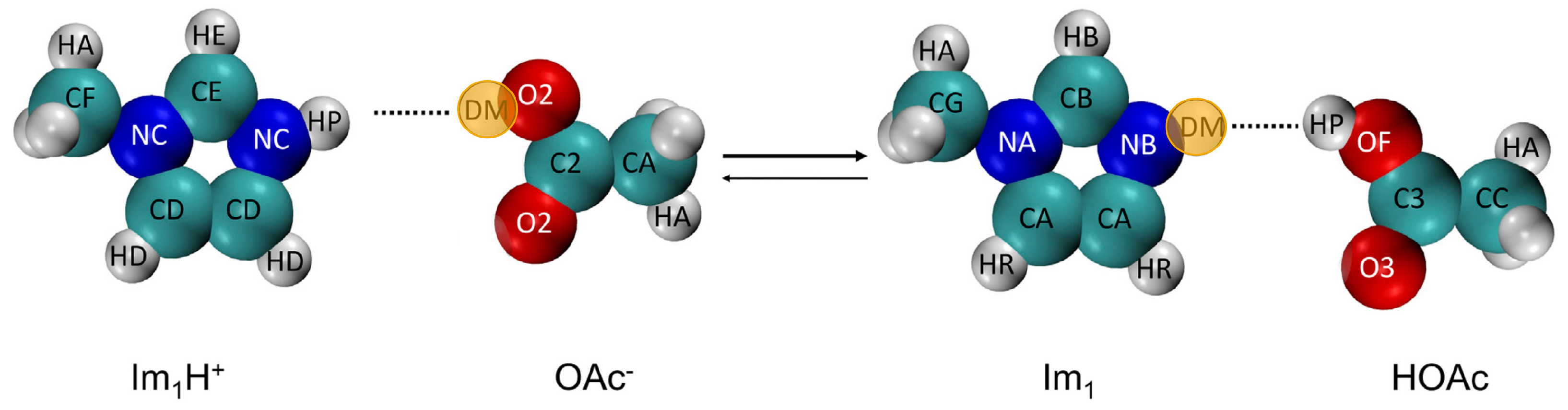
2.3. How to Include Chemical Reactions?

The observed reduction in partial charges may arise not only from the polarization of cations and anions but also from charge transfer [72,91,92,93]. Distinguishing clearly between these mechanisms remains challenging [93]. In fact, fluctuating charges represent one of the algorithms for implementing polarizable force fields [56,94,95,96]. Typically, charge transfer is constrained within individual molecules and not permitted between them to ensure the stability of simulations. This restriction is particularly critical for charged systems such as ILs. However, inter-molecular charge transfer is sometimes allowed, effectively modeling charge transfer reactions. We showed [97] in 2020 (see Figure 3) that enabling charge transfer does not significantly alter the structural and dynamic properties compared to polarizable simulations. Furthermore, charge transfer simulations can be implemented using the previously described topology files, requiring only the addition of a file specifying transient partial charges. In addition, E/Z-isomerization reactions [98,99] can be sufficiently described without the need for explicit changes in bonding. The dissociation and formation of covalent bonds, however, require new approaches. These approaches can be divided into three categories: QM-based methods, continuous force fields, and fractional force fields.

2.3.1. Quantum-Mechanical-Based Methods

Ab initio molecular dynamics simulations (AIMD) were first applied by Lynden-Bell and co-workers for imidazolium-based ILs in 2005 [70,100], as depicted in the timeline of Figure 3. Unlike conventional MD simulations, AIMD calculates forces directly from electronic structures using density functional theory (DFT) [101,102]. This allows for simulations of bond breaking and formation, electronic polarization, charge transfer, and other inherently QM phenomena [103]. In contrast to classical MD, their AIMD studies indicated that the chloride anions are preferentially located near the acidic H2 of the imidazolium ring and participate in directional hydrogen bonding. They suggested that classical force fields should incorporate local dipole moments (like in AMOEBA) to improve the force fields [100].

Kirchner and co-workers [104,105] reported a Grotthuß-like mechanism for 1-ethyl-3-methylimidazolium tetrachloroaluminate dissolved in aluminum chloride. AlCl₃ forms dimers with AlCl₃ and AlCl₄⁻, which attack other Al₂Cl₆ to form a tetrameric species Al₄Cl₁₃⁻ to counteract the electron deficiency:

$$\begin{array}{ccc}{AlCl}_3+{\mathrm{AlCl}}_3& \rightleftharpoons & {Al}_2{\mathrm{Cl}}_6\end{array}$$

(3)

$$\begin{array}{ccc}{AlCl}_3+{{AlCl}_4}^{-}& \rightleftharpoons & {Al}_2{{Cl}_7}^{-}\end{array}$$

(4)

$$\begin{array}{ccc}{Al}_2{{Cl}_7}^{-}+{Al}_2{Cl}_6& \rightleftharpoons & {Al}_4{{Cl}_{13}}^{-}\end{array}$$

(5)

The Grotthuß mechanism involves attacks from chloride on the tetrameric species, which releases one of its chloride atoms. The chloride rattling (with bond breaking and reformation) and its diffusion play a key role in forming and transforming larger anionic species [104], which were also detected experimentally.

A Grotthuß-like mechanism, like that in Figure 5a,b, was reported by another AIMD study of the Kirchner group [31] for the liquid 1-methylimidazole and acetic acid, partially forming the protic ionic liquid 1-methylimidazolium acetate. Although protons may hop between the imidazolium nitrogen and acetate oxygen atoms, the proton conduction occurs predominantly through hydrogen bond rearrangements in extended molecular chains according to the Grotthuß mechanism, with acetic acid molecules acting as primary participants. Chains up to four molecules long were observed, where proton transfer is enabled by simultaneous proton donation and acceptance by acetic acid molecules [31]. Functional group modifications on cations and anions influence proton transfer energetics, providing insights for designing optimized protic ILs. Kirchner and co-workers showed that the Grotthuß mechanism leads to faster proton transport than the slower vehicle mechanism depicted in Figure 5c. These AIMD results confirm high proton conductivity, even though the mixture predominantly comprises neutral molecules.

Bodo and co-workers [103,106,107] conducted AIMD studies on choline systems and reported on multiple proton transfers within the choline-cysteine system, including intramolecular proton transfer within the cysteine anion. However, while their study successfully identified structural properties from noisy radial distribution functions and structure factors, it did not provide detailed dynamical properties, such as diffusion coefficients [103,106]. In subsequent studies, Bodo et al. [103] reported that shared protons between donor and acceptor species contribute significantly to the cohesive forces in these ILs. The dominant interactions combine electrostatic forces with strong hydrogen bonds to overcome the natural electrostatic repulsion between anions. This is facilitated by charge delocalization and dielectric screening within the ionic medium [107]. Proton migration mechanisms in these systems depend on the specific functional groups involved. Migration is reversible between carboxylate and phosphate groups, suggesting dynamic equilibrium. In contrast, when an amino group accepts the proton, the migration process becomes effectively irreversible, forming zwitterionic species. This behavior ultimately quenches proton transfer and reduces the overall ionic conductivity of the fluid [107]. Bodo highlighted the potential formation of zwitterionic anions through secondary proton transfer processes, transforming amino acid anions into unconventional isomeric forms. This structural evolution has implications for the conductivity and electrochemical behavior of amino-acid-based ILs, as well as their application in CO₂ capture and other chemical processes [107].

The Kirchner group [108] noticed strong fluctuations of the C2-H2 bond in aprotic 1-ethyl-3-methylimidazolium, suggesting that this bond is almost broken and the acetate anion accepts the hydrogen. Adding water to the IL makes proton abstraction less probable. The acetate anion forms strong hydrogen bonds with water that can lead to the abstraction of a proton from the water molecule. Hollóczki et al. [109,110] and Kirchner et al. [110,111] showed that the remaining cations stabilize the carbene via strong hydrogen bond interactions if the cation in Figure 1 gets deprotonated. The strongest hydrogen bonds are detected for the H2 ring imidazolium hydrogen to the carbene. Interestingly, the hydrogen bonding between the methyl-hydrogens and the carbene is stronger than the other ring hydrogens H4 and H5. Hollóczki et al. [109] noticed that the position of the equilibrium in Figure 1 noticeably depends on the basis set used, favoring the right-hand side when increasing its complexity. Since the AIMD studies [110,111] used only one carbene and acetic acid molecule, the actual ratio between the IL 1-ethyl-3-methylimidazolium acetate and its carbene/acetic acid counterparts is still unclear. In addition, AIMD simulations cannot be performed with a wide range of CO₂ composition, which would be necessary to study the pressure dependence of the reactions. On the other hand, these AIMD simulations are currently the only theoretical approach that handles carbene formation and can observe the chemisorption of one CO₂ molecule.

AIMD simulations are inherently constrained by their high computational costs, allowing for the study of only a limited number of ion pairs (typically tens) over short simulation periods, usually spanning a few dozen picoseconds. As a result, the insights gained are restricted to the behavior of a small local environment, such as an ion pair undergoing proton exchange surrounded by a few neighboring cations and anions.

Figure 6a illustrates the issue: Consider dividing a cubic simulation box into 27 equal cells by partitioning each spatial dimension into three segments. In typical AIMD simulations, only one ion pair occupies each of those cells. Consequently, the ion pair on the right side of the central cell simultaneously serves as a neighbor for the ion pair on the left side of the central cell. This artificial periodicity creates limitations [112] in accurately capturing the larger-scale nanostructures of ILs, such as the formation of oscillating cation-anion layers [113,114,115] or polar and apolar domains [54], which arise from the interplay of short-range dispersion forces and long-range Coulombic interactions and extend over tens of Ångströms [33,56,116]. Furthermore, the small box size also restricts proton hopping pathways. Moreover, AIMD simulations often suffer from significant noise in radial distribution functions [70,100,103,106], and dynamical properties like diffusion coefficients and conductivity are infeasible to compute [112]. Given these constraints, hybrid approaches have emerged as promising alternatives. By combining QM methods for the chemically reactive region with classical MD to represent the surrounding solvent molecules (see Figure 6b), these methods achieve a balance between computational efficiency and accuracy. Such hybrid multiscale techniques enable the exploration of larger systems while retaining the ability to capture critical chemical reactivity and solvent effects at the molecular level [117,118,119]. However, only non-polarizable force fields are applied for the MD part [118], which might cause problems because of overestimating Coulomb interactions in ILs [56]. Furthermore, at the interface of the QM and the MD region, the flexible electron density of the QM region is in contact with the fixed partial charge distribution of the MD region, which might also introduce simulation artifacts. Multiscale schemes can be classified based on how electrostatic interactions are treated [120,121]: In “mechanical embedding”, QM calculations are performed in the absence of the MD subsystem, and the electrostatic interactions are computed at the MD level using point charges. In contrast, “electrostatic embedding” includes the influence of the MD subsystem’s electrostatic field in the QM calculations. Permanent multipoles of MD atoms are incorporated into the QM Hamiltonian, allowing the polarization of the QM region. “Polarized embedding” extends electrostatic embedding by incorporating classical polarization models to account for mutual polarization between QM and MD regions. “Flexible embedding” allows for mutual polarization and partial charge transfer between QM and MD regions in a self-consistent manner and represents the most advanced and computationally demanding approach [122]. The “ONIOM” ("our own N-layered integrated molecular orbital and molecular mechanics") approach [123] partitions hybrid multiscale systems into multiple layers, allowing for a more refined treatment of the surrounding molecular environment. In principle, the method can also accommodate QM/QM models, wherein electronic effects and reactions are permitted to extend across the layer boundaries, enhancing the accuracy of the representation of interfacial interactions.

Acevedo and colleagues [118,124,125] demonstrated the reliability of multiscale methods across diverse solvent systems (hydrocarbons, water, ILs). Their work included applications to a wide range of organic reactions, such as substitutions [126], eliminations [127], and pericyclic reactions [128].

The Diels–Alder cycloaddition represents another example of an important organic reaction, which has been the object of extensive experimental and theoretical investigations (see Figure 7 taken from Ref. [117]), and the effect of IL structure has been evaluated on product selectivity and reactivity [117]. The capacity of ILs to act as hydrogen bond donors, predominantly influenced by the cation, is tempered by their hydrogen-bond-accepting capabilities, which are primarily dictated by the anion. This interplay was investigated in the context of solute–solvent interactions within acidic and basic chloroaluminate melts [128], focusing on key stationary points along the reaction coordinate of the Diels–Alder reaction between cyclopentadiene and methyl acrylate. A foundational supermolecular model incorporating the 1-ethyl-3-methylimidazolium cation was initially employed, later extended to include the aluminum-based anions AlCl₄⁻ and Al₂Cl₇⁻. Systems containing two anions and one cation were also explored using multiscale calculations and a Monte Carlo algorithm for the dynamics, albeit with reduced accuracy to accommodate larger configurations. The results corroborated prior DFT findings, revealing that the acidic anion Al₂Cl₇⁻, prevalent under excess Lewis acid conditions, exhibits weaker ion-pairing with the imidazolium cation compared to the basic AlCl₄⁻ anion. This diminished ion-pair interaction in acidic media enhances the accessibility of the imidazolium for coordination with the dienophile’s carbonyl group during the transition state (see Figure 7), contributing to the observed rate acceleration. Specifically, the study challenges the conventional emphasis on the hydrogen at the C2 position of imidazolium as the principal hydrogen bond donor. Instead, the more sterically accessible hydrogens H4 and H5 were identified as pivotal in stabilizing the transition state through enhanced hydrogen bonding. The findings provide a detailed molecular-level understanding of how the ionic composition and interactions within the IL influence reactivity. The weaker ion pairing in acidic melts reduces the energetic barriers, stabilizing the transition state more effectively. This mechanistic insight aligns with experimental observations of increased reaction rates and selectivities in acidic chloroaluminate melts compared to their basic counterparts, water, and nonpolar solvents.

By employing conventional force fields to model the surrounding solvent molecules and limiting the QM treatment to a small reactive region, the number of molecules and the accessible simulation length can be increased significantly by an order of magnitude (see Figure 6b). However, the studies conducted by Acevedo [118,124,125,126,127,128], as discussed herein, predominantly utilize a Monte Carlo scheme to generate new molecular configurations. As a result, these studies do not involve a defined simulation period, making direct comparisons with other methods in terms of time-dependent properties infeasible. Despite these advances, the reactive region in such simulations remains limited in size (maybe even smaller than in the AIMD simulations), prohibiting the exploration of phenomena such as the Grotthuß mechanism’s impact on ionic conductivity. Similarly, diffusion-controlled processes, such as CO₂ absorption, remain inaccessible due to the inherently low diffusion coefficients and the constrained simulation timescales in QM and multiscale simulations. These limitations hinder the sufficient exchange of molecular environments. The reactive region often contains very few (or even a single pair of) reacting molecules. Nonetheless, QM and multiscale simulations excel in elucidating reaction pathways, providing critical insights into the mechanistic details of chemical transformations.

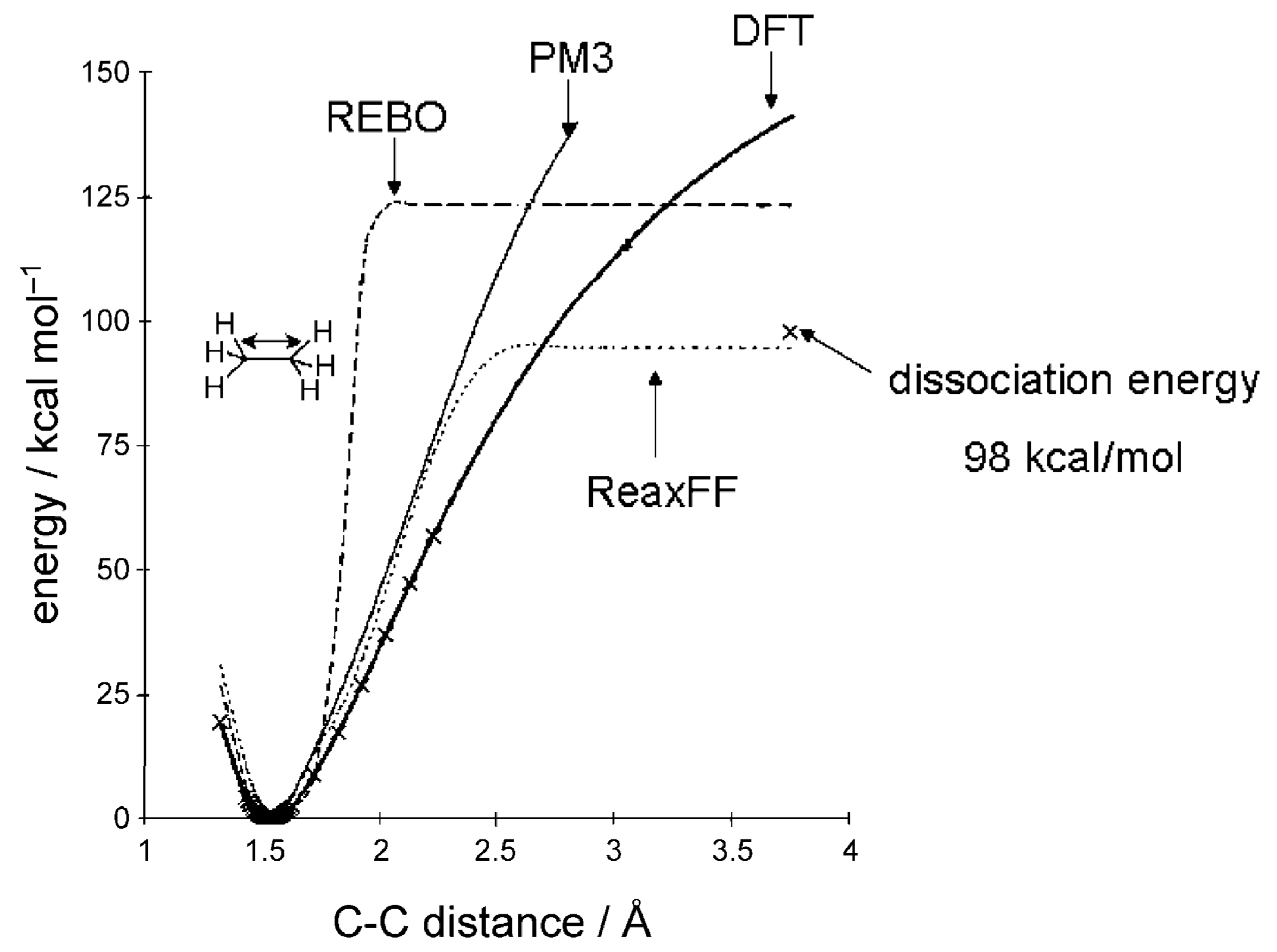
2.3.2. Continuous Force Fields

Reactive force fields enable a substantial expansion of the reactive region, potentially extending across the entire simulation box. However, conventional MD simulations [16,77,80,81], which rely on fixed protonation states, are inherently limited in capturing the dynamic proton transfer processes characteristic of protic ILs. Although constant-pH simulations [129] incorporate a dynamic protonation mechanism that allows for exploring variable protonation states based on local acidity or basicity, these methods are primarily designed for systems with limited titratable sites, such as proteins, and become computationally prohibitive as the number of titratable sites increases. This computational overhead renders constant-pH simulations impractical for protic ILs, where hundreds of cations and anions are subject to frequent protonation and deprotonation events.

The “empirical valence bond” (EVB) model by Warshel [130] provides another framework in MD simulations for modeling chemical reactivity by incorporating resonance structures and is based on the following secular determinant:

$$\left|\begin{array}{cc}{U}_1-E& U_{12}\\ U_{12}& U_2-E\end{array}\right|=0$$

(6)

where $U_1$ and $U_2$ represent the empirical force-field-derived energies of the reactant and product states, respectively [131]. The coupling term $U_{12}$ mediates the transition between these states and can be parameterized using experimental or QM data, such as transition state barrier heights $\Delta E$. Chang and Miller [132] introduced generalized Gaussian functions to express the $U_{12}$ term. Subsequent improvements were proposed by Kim et al. [133] and Schlegel and Sonnenberg [134]. The energy E corresponds to the current status of the chemical reaction. By diagonalizing this 2 × 2 matrix in Equation (6), reactive processes can be efficiently modeled with standard force fields [55,131,135]. EVB models have found widespread application in simulating chemical reactions involving hydrogen transfer. For instance, Hinsen and Roux investigated the intramolecular proton transfer in the enol form of acetylacetone [136]. Similarly, Nagaoka et al. [137] and Okuyama-Yoshida et al. [138] studied the proton transfer reaction of glycine in aqueous solution. Luzhkov explored hydrogen transfer during the peroxidation of phenol [139]. Comparisons of proton transfer reactions in solution and enzymes have also been extensively conducted, demonstrating the model’s adaptability [130,140,141,142]. Like the multiscale method [119,126,143], the strength of the EVB model lies in its flexibility to incorporate solvent effects [130]. Its influence on reacting centers is introduced and fine-tuned through the diagonal terms of the determinant in Equation (6). However, EVB does not inherently support dynamic bond breaking and formation and is usually limited to a single reaction. Voth and coworkers extended the EVB approach to a multi-state model describing proton transfer in aqueous solutions [144,145]. It was refined in the early 2000s [142,146,147,148], including proton transfers involving imidazolium and water [149]. Otherwise, only two publications exist on the valence bond theory of protic ILs. However, they deal with the ab initio valence bond, not the EVB model [150,151].

Alternatively, bond-order potentials such as the Tersoff potentials [152,153,154,155] or the reactive force field ReaxFF developed by van Duin et al. [156,157,158] provide a framework for MD simulations that dynamically form and break chemical bonds. Tersoff potentials are designed explicitly for covalent systems with fixed bond types and limited reactivity, focusing primarily on bonded interactions in materials like silicon and carbon-based structures [152,159]. The optimization of short-range interactions in hydrocarbons, accurately describing single, double, and triple carbon–carbon bonds, led to the development of the “reactive empirical bond order” (REBO) force field in 1990 [55,159]. However, REBO lacks long-range interaction terms [155], making it unsuitable for systems dominated by nonbonded interactions, such as ILs. Additionally, the inability to account for torsional interactions further limits its applicability, particularly in polymeric systems. In 2000, Stuart et al. [155] extended the REBO framework by introducing the “adaptive intermolecular reactive empirical bond order” (AIREBO) force field, which addresses many of REBO’s limitations. AIREBO incorporates long-range interactions through a Lennard–Jones potential and torsional flexibility via cosine-based terms [152]. These long-range interactions are smoothly introduced or turned off during reactions using switching functions [155], thereby preserving the reactive nature of the potential. While AIREBO significantly improves upon REBO, it is computationally more demanding. Although issues related to nonbonded interactions have been mitigated, AIREBO remains less effective than conventional force fields optimized for long-range interactions. A further limitation of both AIREBO and REBO is that they do not work with atom types [160]. Unlike classical empirical force fields, this approach necessitates system-specific parameterization, requiring refitting and revalidation for new chemical environments. This lack of transferability increases the complexity of their implementation and poses significant challenges for simulations involving diverse chemical systems. Such extra efforts are particularly frustrating when the chemical reactions modeled are not the primary focus but merely a secondary aspect of a broader simulation study. In contrast to EVB, AIREBO handles bond breaking and formation dynamically. It has been applied since 2015 to describe the flexibility of graphene surfaces in contact with 1-butyl-3-methylimidazolium-based ILs [161,162], which were treated by conventional non-polarizable force fields.

The “reactive force field ” (ReaxFF) [156,157,158,163] represents a significant advancement over traditional bond-order potentials like REBO and AIREBO by incorporating long-range interactions and dynamic bond formation and dissociation. The potential energy function $U_{ReaxFF}$ augments the traditional energy in Equation (2) by additional correction terms [55]:

$$U_{ReaxFF}=U_{FF}+U_{coordination}+U_{conjugation}+U_{lonepair}+U_{HB}$$

(7)

Each additional term addresses specific aspects of bonding and molecular interactions, ensuring the accuracy and flexibility of the potential. The coordination energy $U_{coordination}$ addresses stability issues associated with bonding configurations that deviate from ideal coordination environments, such as strained geometries or configurations involving adjacent double bonds. This term imposes a penalty on atoms that exceed their expected valence by forming an excessive number of bonds, thereby preventing non-physical configurations. Conversely, it stabilizes atoms with fewer bonds than their typical valence, accounting for resonance effects observed in radicals or conjugated systems. The conjugation correction $U_{conjugation}$ accounts for bond rotation effects in aromatic hydrocarbons, ensuring that resonance stabilization is adequately captured. The energy contribution $U_{lonepair}$ represents the interactions associated with electron lone pairs, which can significantly influence the hydrogen bonding interactions described by $U_{HB}$. In conjunction with the dynamic computation of bond orders [158], these corrections enable ReaxFF to accurately represent reaction barriers and capture the complex behavior of reactive systems, including ILs [55]. ReaxFF also incorporates a comprehensive treatment of non-bonded interactions, essential for modeling systems where long-range forces play a significant role, such as in ILs. Non-bonded interactions between all atom pairs, including first, second, and third neighbors, are explicitly included in the model. Van der Waals interactions are described using a “shielded” Morse potential, where distance-dependent screening attenuates short-range interactions. Similarly, Coulombic interactions are screened to maintain accuracy for closely spaced atoms. ReaxFF eliminates the need for switching functions, ensuring a smooth and seamless transition between bonded and non-bonded interactions. This capability allows ReaxFF to accurately capture the interplay of long-range forces and dynamic bonding, which is critical for studying complex chemical processes. Nevertheless, ReaxFF is limited close to equilibrium [164] due to the restricted treatment of non-bonded interactions. Additionally, ReaxFF does not rely on predefined atom types, unlike many classical empirical force fields, and instead requires extensive QM calculations for parameterization. While this approach enhances its versatility, it also increases the computational effort required for its use. Moreover, the parameters developed for one environment, such as an aqueous phase, are not inherently transferable to others, such as gaseous systems. This lack of transferability further complicates the application of ReaxFF across diverse chemical environments. Nevertheless, the results from ReaxFF often show better agreement with AIMD simulations than those from REBO, highlighting its accuracy and reliability [165]. The capabilities of ReaxFF have been demonstrated in numerous studies, like for forming an electric double layer [166] and lubricant processes [167]. Johnson et al. [168] applied ReaxFF to simulate a system containing 50 tetrabutylphosphonium glycinate and 25 CO₂ molecules over a 2 $\mathrm{n}$$\mathrm{s}$ period to investigate the reaction pathways. Their simulations revealed extremely low energy barriers, below 2 kcal mol⁻¹, for proton transfer and chemisorption processes. The study also observed a steeper density increase during CO₂ uptake compared to AIMD simulations, and multiple proton transfer events were recorded, which were not observed in AIMD [168]. These findings underscore the ability of ReaxFF to model dynamic chemical processes and to capture subtle molecular interactions that are difficult to observe experimentally or through other computational approaches. ReaxFF is implemented in LAMMPS [169] via the “pair_style reaxff” command.

The “interface force field” [170] replaces harmonic bond potentials of reactive bonds with energy-conserving Morse potentials instead of bond-order potentials. This modification enables the accurate simulation of bond dissociation and formation while maintaining seamless compatibility with widely used force fields such as CHARMM, GAFF, OPLS-AA, and AMBER. The framework of the interface force field is highly computationally efficient, offering a 30-fold speed improvement over ReaxFF while achieving comparable or superior accuracy across diverse material systems. Moreover, the shifted Morse potentials in the interface force field facilitate bond dissociation modeling with fewer parameters than ReaxFF, which are both simpler to parameterize and more interpretable. The interface force field is compatible with established non-reactive force fields and preserves their parameterization for non-reactive properties, thereby eliminating the need for multiple parameter sets and simplifying its implementation. In contrast, ReaxFF relies on more complex potential functions, which allow for the modeling of intricate reaction pathways but come with significantly higher computational costs for trajectory production and analysis. To date, the interface force field has been successfully applied to polymer systems and carbon nanotubes [170], but its application to ILs remains unexplored.

2.3.3. Fractional Force Fields

Reactive molecular dynamics approaches often require modifications at the fundamental level of trajectory production. As a result, conventional MD programs known for their computational efficiency, such as CHARMM, AMBER, GROMACS, and OpenMM, are typically incompatible with these methods. Instead, less efficient, often custom-written code is needed to handle the non-conventional potentials associated with reactive simulations, which can limit the total simulation time and system size. While some studies focus on specific reaction pathways between individual reacting molecules, many others are primarily interested in broader phenomena where reactions form only one component of a more extensive system. For instance, in investigations of the conductivity of protic ILs, the focus is not on the detailed mechanism of individual acid-base reactions but on the cumulative effect of thousands of proton transfer events on the system’s overall conductivity [171]. For such studies, it is often sufficient to model transitions between reactants and products with physically meaningful transition probabilities [86] rather than explicitly resolving every reaction at the QM level. When the reactions anticipated within a system are known in advance, a practical alternative involves manually interrupting the simulation to modify the system’s topology by transitioning from a reactant-based to a product-based force field [160,171,172]. Unlike traditional reactive force field approaches, this method results in discontinuous trajectory production, and we refer to such force fields as “fractional force fields”. They have been successfully employed in various studies, including the in situ generation of equilibrated polymer structures, investigations into chain and cross-linking polymerization processes [55], and the modeling of proton hopping mechanisms [171,173].

In classical MD simulations, bonds, valence angles, dihedral angles, and atomic charges are predefined at the start of the simulation and remain constant throughout its duration. This approach facilitates using straightforward data structures (as illustrated in Figure 2) and efficient memory management for static interaction lists. In contrast, reactive force fields necessitate dynamic updates, as bonds may form or break, and three-body and four-body interactions must be recalculated at every timestep within continuous force fields. This lack of a fixed topology significantly complicates both memory management and trajectory analysis. Fractional force fields address these challenges by maintaining stable data structures during regular production simulations, similar to classical MD. Updates to the topology are only performed when the simulation is paused to evaluate potential reactions.

Figure 8 illustrates the proton transfer from 1-methylimidazolium acetate [Im₁H]OAc to form 1-methylimidazole Im and acetic acid HOAc, using the single topology approach within the Python-based PROTEX program [171,172]. The term “single topology” originates from alchemical free energy calculations [174] and describes a method where both the initial and final states of a molecular system are represented by a single set of molecular topology parameters. This single representation enables transitions between the two states by scaling or interpolating relevant parameters, such as atomic charges, Lennard–Jones parameters, or intramolecular force field terms:

$$E=(1-\lambda )U_1+\lambda ·U_2$$

(8)

In this formalism, $\lambda =0$ corresponds to the situation of the reactants, whereas $\lambda =1$ refers to the product state. Like in the EVB model, E characterizes the current status of the reaction. For proton transfer reactions in ILs conducted by PROTEX [171,172], we only used $\lambda =0$ and $\lambda =1$ but no states in between to avoid non-physical intermediate steps in the trajectory. During the proton transfer reaction, the PROTEX program [171,172] transforms the hydrogen atom HP of 1-methylimidazolium Im₁H⁺ into a dummy atom (DM) within the 1-methylimidazole Im₁ molecule. Simultaneously, the DM atom of the acetate OAc⁻ is converted into the HP atom of acetic acid on the product side of the reaction, as depicted in Figure 8. Nevertheless, as shown in Figure 2, the dummy atoms still exist in the list of the topology file (as a placeholder). This method simplifies the handling of topology files during trajectory analysis using tools like MDAnalysis [62,175], as molecules can be addressed through a fixed set of atom indices in the topology file, ensuring consistency throughout the simulation. Reactive MD simulations using PROTEX [171,172] offer the capability to accurately model the conductivity of protic ILs, enabling the study of mechanisms such as the Grotthuß proton transfer. Additionally, PROTEX [171,172] supports the simulation of charge transfer processes and keto-enol tautomerism reactions. It can also model the deposition of compounds onto (electrode) surfaces, including passivation phenomena. However, PROTEX [171,172] is primarily suited for reactions involving the exchange of small moieties, such as protons. While it is still capable of simulating processes like the chemisorption of CO₂, it is not suitable for more complex reactions, such as cross-linking in polymers, which require modeling larger structural transformations.

An alternative to PROTEX is the REACTER module [176,177,178] within the MD program LAMMPS, which leverages the program’s unique topology structure to enable the simulation of reactions in MD frameworks. REACTER [176,177,178] employs a superimpose algorithm capable of efficiently identifying local topology patterns on an atom-to-atom basis by utilizing predefined templates and distance criteria. This method allows for the representation of complex reactions, such as polymerization, with high computational efficiency. However, REACTER [176,177,178] does not incorporate a dedicated strategy for determining the acceptance probability of reactive steps, a crucial component for modeling reactions in a physically accurate manner. The analysis of trajectories generated by REACTER [176,177,178] is not straightforward using MDAnalysis [62,175]. Instead, the open-source Python package LUNAR [179] (LAMMPS Utility for Network Analysis and Reactivity) is recommended. It is a comprehensive toolkit specifically designed for LAMMPS, enabling efficient MD model building, simulation, and analysis to accurately establish structure–property relationships in polymers and polymer composites. LUNAR [179] provides key features tailored to reactive LAMMPS simulations, including automatic assignment of atom types, incorporation of higher-order interactions, calculation of partial charges for classical force fields, and the generation of input files required for the REACTER [176,177,178] protocol. Additionally, it supports initial configuration setup and includes advanced analysis routines relevant to dynamic polymer networks, such as cluster analysis and free volume calculations.

A notable drawback of fractional force fields is their potential failure to conserve energy when switching from the potential energy surface of the reactants (characterized by $U_1$) to that of the products (characterized by $U_2$). However, several strategies can be employed to address this issue: First, in “adiabatic reactive molecular dynamics” (ARMD) [180,181,182], reactions occur in MD simulations when the energy difference $\Delta U=(U_1+\delta U)-U_2$ changes the sign. The inclusion of an asymptotic separation term $\delta U$ ensures that $U_1+\delta U$ and $U_2$ share a common zero energy reference. This approach eliminates discontinuities in the energy profile at the moment of reaction, providing a smooth transition between reactant and product energy surfaces. ARMD [180] may also make use of Equation (8) to increase the control of the reaction. Second, for cases where reactions are determined by geometric criteria rather than energetic considerations, additional potentials, such as those employed in rs@md [160], can be introduced to ensure continuity. Third, in PROTEX [171,172], the number of $\lambda$-states may be increased to smoothen the transition. Fourth, polarizable simulations are also beneficial [171] and are a prerequisite for using PROTEX. In the case of proton transfer in protic ILs, charged molecules transition to neutral states or vice versa, leading to abrupt changes in Coulombic energy. This behavior arises because neutral molecules exhibit significantly weaker electrostatic interactions compared to charged species. Moreover, the partial charge distribution of the product molecules typically differs from that of the reactant molecules. Polarizable force fields mitigate these challenges by incorporating induced dipoles, which dynamically adapt to changes in the Coulombic environment, thereby effectively smoothing transient energy fluctuations and enhancing the stability of the simulation [171]. In contrast, Lennard–Jones parameters, which account for van der Waals interactions, typically exhibit minimal variation between reactant and product states. Consequently, no significant issues are expected from these parameters during transitions, simplifying their treatment in reactive simulations using fractional force fields.

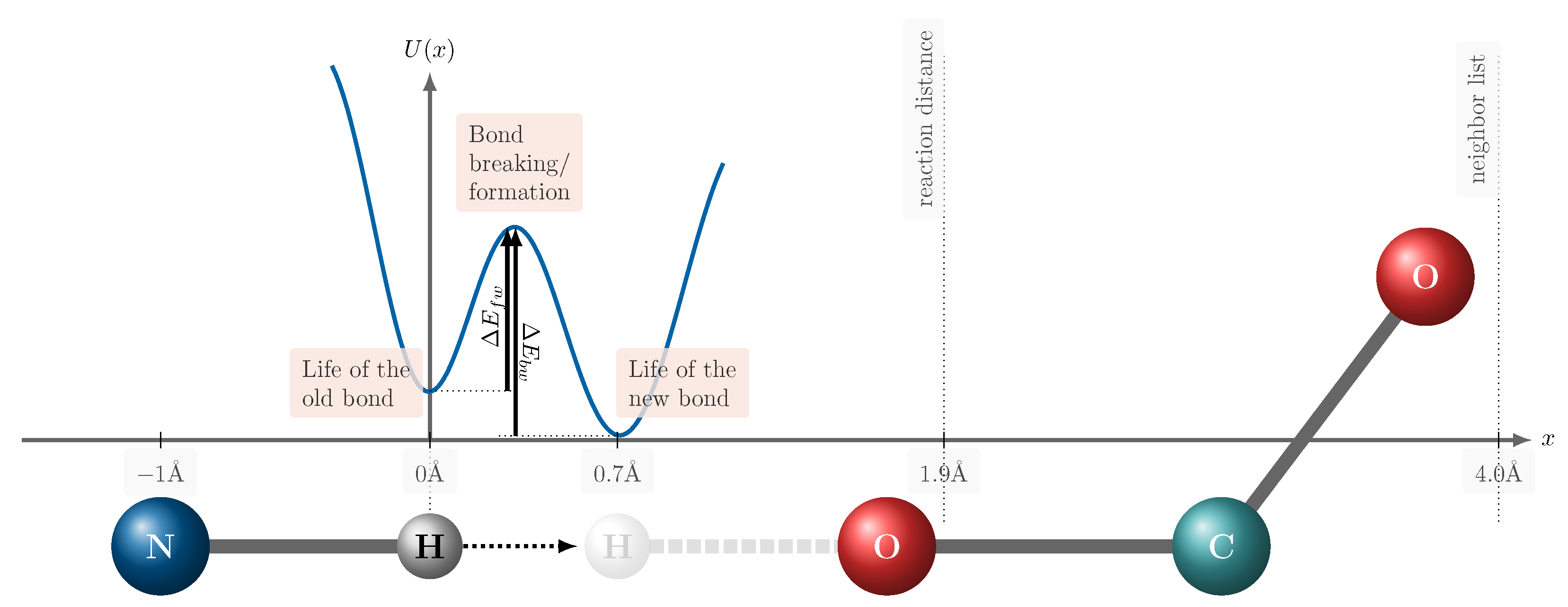
3. Modelling the Reaction

Not all of the aforementioned approaches in reactive dynamics have been specifically applied to ILs. However, they have been discussed here to provide a comprehensive overview of the possibilities available in reactive MD simulations. The methods that have been employed in the context of ILs are highlighted in the yellow-shaded region of Figure 3, along with the year of their first application to IL modeling, though the methodologies themselves may have been developed much earlier.

In this section, we aim to compare and contrast the workflows and algorithms of reactive continuous and fractional MD approaches to elucidate their differences, advantages, and limitations. Figure 9 illustrates the proton transfer mentioned in Figure 8 as an example of a typical reaction. At first glance, the depicted energy profile appears to be significantly compressed. However, this is a result of the reaction coordinate x undergoing only a small change relative to the dimensions of the bonds and the reacting molecules. In Figure 8, the reaction coordinate represents the position of the hydrogen atom during the proton transfer, measured with respect to the equilibrium position of the old bond being broken. Geometric criteria for identifying reaction partners are typically set to distances below $1.9$ Å. For proton transfer reactions, hydrogen bonds are usually a prerequisite, implying that the distance between the two electronegative atoms involved (here nitrogen and oxygen) must be less than 3 Å. Additionally, the ReaxFF force field requires a neighbor list to compute Coulomb and Lennard–Jones interactions, which should extend approximately 4Å to 5Å around the reacting atom (in this case, hydrogen). The discontinuity in fractional MD simulations is the “jump” of the hydrogen from x = 0 Å (the equilibrium position of the old bond) to $0.7$ Å, which is the position of the equilibrium of the new bond. Our discussion is structured around three key phases of the reaction process: the life of the initial bond, the bond-breaking and formation transition, and the life of the newly formed bond. This framework allows for a systematic examination of each approach’s methodologies and their implications for reactive MD simulations.

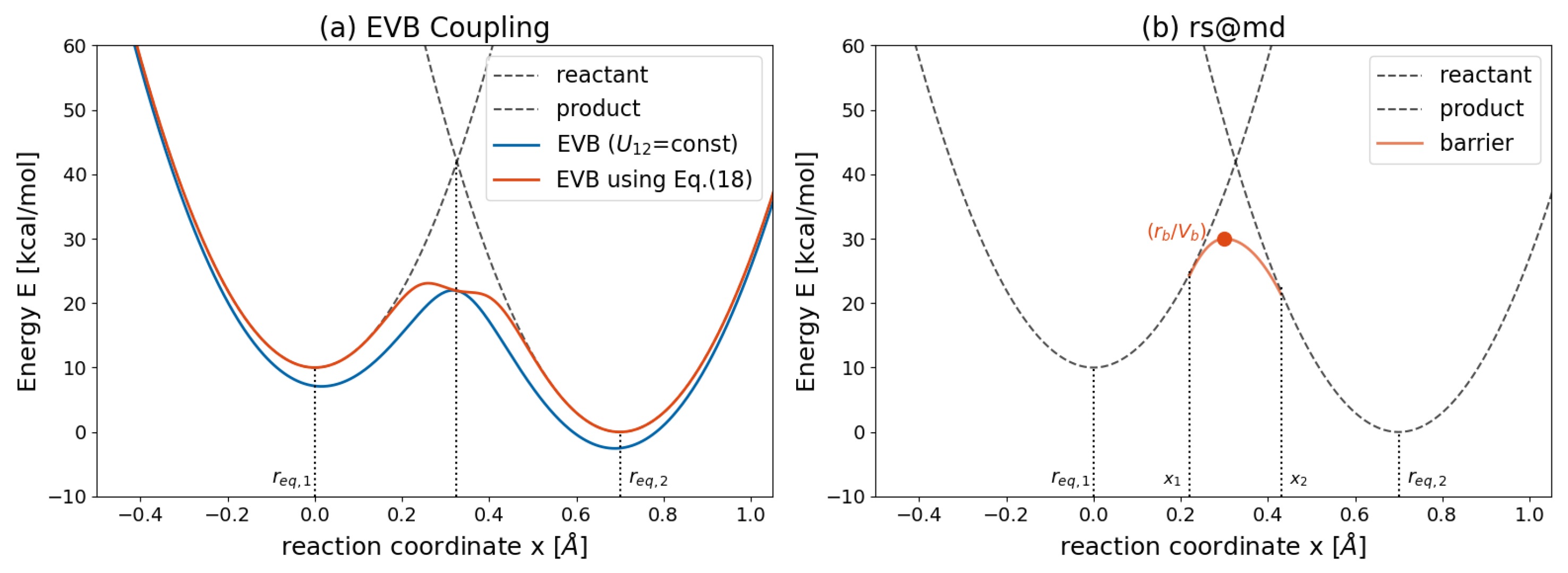
3.1. Life of the Old Bond

In classical force fields, bonds are usually modeled by a harmonic potential:

$$U_{bond}\left(r\right)=k_{bond}(r-r_{eq}{)}^2$$

(9)

The difference between the actual distance of the two atoms r and its equilibrium value $r_{eq}$ is x in Figure 9. The actual values of the equilibrium bond length $r_{eq}$ and the force constant $k_{bond}$ depend on the nature of this bond and may be different from those values of the new bond. The harmonic bond potential is part of classical force fields and is consequently used by PROTEX [171,172]. When a bond is expected to dissociate, the harmonic potential can be replaced by a Morse potential,

$$U_{bond}\left(r\right)=D(1-exp[\alpha (r-r_{eq})]{)}^2$$

(10)

which has a dissociation energy of D. The curvature $\alpha$ describes the steepness of the potential. Expanding Equation (10) in a Taylor series around $r_{eq}$ recovers the harmonic potential of Equation (9) with $k_{bond}=D{\alpha }^2$. Morse potentials are used in the interface force field [170] and the adiabatic reactive force field (ARMD) [180,181,182], the latter of which also retains harmonic potentials [180]. The REBO method [159] employs an attractive potential $U_{attractive}\left(r\right)$ and a repulsive potential $U_{repulsive}\left(r\right)$, both of which resemble Morse potentials, to model bond energies:

$$\begin{array}{ccc}\hfill U_{repulsive}\left(r\right)& =& {\displaystyle \frac{f\left(r\right)}{S-1}}D·exp\left[-{\alpha }_1(r-r_{eq})\right],\hfill \end{array}$$

(11)

$$\begin{array}{ccc}\hfill U_{attractive}\left(r\right)& =& {\displaystyle \frac{f\left(r\right)S}{S-1}}D·exp\left[-{\alpha }_2(r-r_{eq})\right],\hfill \end{array}$$

(12)

$$\begin{array}{ccc}\hfill U_{bond}\left(r\right)& =& U_{repulsive}\left(r\right)-B·U_{attractive}\left(r\right).\hfill \end{array}$$

(13)

The switching function $f\left(r\right)$ ensures that the potentials are limited to interactions between nearest neighbors [159]. Furthermore, the relationship between these potentials is modulated by an empirical bond-order function B.

The bond order is not a parameter in these potentials but can be deduced from the equilibrium distances $r_{eq}$ and force constants $k_{bond}$. For example, the bond distances for a carbon–carbon single, double, and triple bond are roughly $1.5$ Å, $1.3$ Å, and $1.1$ Å, respectively. The force constant $k_{bond}$ should increase with bond order. The actual values depend on the immediate local environment and are tabulated in daily used force fields. Chemical intuition argues for integer values of the bond order. However, in ReaxFF [158,165], the bond order $BO\left(r\right)$ is a continuous function of the distance r between the two atoms i and j:

$$\begin{array}{ccc}\hfill B{O}_{type}^{\prime }\left(r\right)& =& exp\left[a_{type}{\left({\displaystyle \frac{r}{r_{type}}}\right)}^{b_{type}}\right]\hfill \end{array}$$

(14)

$$\begin{array}{ccc}\hfill BO\left(r\right)& =& (B{O}_{\sigma }^{\prime }\left(r\right)+B{O}_{\pi }^{\prime }\left(r\right)+B{O}_{\pi \pi }^{\prime }\left(r\right))·f({\Delta }_i^{\prime },{\Delta }_j^{\prime },B{O}^{\prime })\hfill \end{array}$$

(15)

$$\begin{array}{ccc}\hfill U_{bond}\left(r\right)& =& -D_{\sigma }·B{O}_{\sigma }·exp\left[p_1\right(1-B{O}_{\sigma }^{p_2}\left)\right]-D_{\pi }·B{O}_{\pi }-D_{\pi \pi }·B{O}_{\pi \pi }\hfill \end{array}$$

(16)

The parameters $a_{type}$, $b_{type}$, and $r_{type}$ are specific to the type of the bond: $\sigma$, single $\pi$, and double-$\pi$ bond. The actual bond order $BO\left(r\right)$ depends on the sum of $B{O}_{\sigma }^{\prime }\left(r\right)$, $B{O}_{\pi }^{\prime }\left(r\right)$, and $B{O}_{\pi \pi }^{\prime }\left(r\right)$. The parameters $p_1$ and $p_2$ are employed to model the unique characteristics of the corresponding single bond. Although the term “life of the old bond” suggests that only the bond potentials, $U_{bond}$, of the reacting pairs are affected in Equation (2), in reality, all intramolecular potentials of those molecules are influenced. Consequently, angle and torsional potentials are also corrected using bond-order terms. The bond order is expressed as a function of the atoms j that share an angle potential with atom i. The correction function, $f({\Delta }_i^{\prime },{\Delta }_j^{\prime },B{O}^{\prime })$, consists of multiple factors that depend on the deviations, ${\Delta }^{\prime }$, of atoms i and j from their optimal coordination numbers, and the uncorrected bond order, $B{O}^{\prime }$ [158,165]. The large number of parameters in Equation (16) highlights the significant parametrization effort in ReaxFF, which becomes even more pronounced when corrections and additional parameters for angles and torsions are included. Moreover, the potential energy is supplemented by contributions from coordination effects, lone pairs, and hydrogen bonding, as indicated in Equation (7). ReaxFF also incorporates transient charges, $q_i\left(t\right)$ [165], which are dynamically distributed within each molecule at every timestep, in a manner analogous to the fluctuating charge model used in polarizable MD simulations [56].

Figure 10 demonstrates the value of this extensive parametrization, as ReaxFF accurately reproduces semi-empirical PM3 results [183] and aligns closely with the experimental dissociation energy of 98 kcal mol⁻¹. In contrast, the corresponding REBO predicts a significantly higher dissociation energy and a steeper energy profile. Similarly, a Morse potential fitted to DFT results fails to replicate the experimental dissociation energy accurately [55,165].

The cutoff for the neighborhood list of bonded interactions in ReaxFF ranges between 4 Å and 5 Å, as indicated by the dotted line in Figure 9. As a result, both oxygen atoms in the acetate group are considered during bond-order calculations. This cutoff is essential as bond orders between all reactive atoms would need to be computed otherwise. For simulations involving 500 ion pairs of ILs, with two to three reactive atoms per molecule, approximately one million bond orders would need to be calculated at each timestep. By applying the cutoff, the list of potential reacting partners is reduced to the ten immediate neighboring molecules.

The analysis of ReaxFF trajectories presents a significant challenge due to the vast number of molecules and fragments involved in numerous chemical reactions. The complexity of these dynamic processes exceeds the capabilities of existing analytical tools and manual examination. To address this limitation, a cheminformatics-based approach, VARMD (visualization and analysis of reactive molecular dynamics) [184], systematically processes and visualizes reaction pathways, molecular interactions, and structural transformations occurring during the simulation.

3.2. Bond Breaking and Bond Formation

In principle, the EVB method operates with classical force fields like in Equation (2). Recently, Grimme combined his “quantum mechanically derived force field” [164,185] with EVB. Unlike classical force fields, Grimme’s force field employs distinctive formulations for bond, angle, and torsional potentials [164], substituting equilibrium distances and angles with QM computed values. Additionally, it incorporates an attractive hydrogen-bonding potential, thereby favoring proton transfer reactions. The reaction energy profile can be modeled using the EVB determinant in Equation (6). The coupling term may either be a constant or derived from the mixing of two bond potentials:

$$U_{12}\left(r\right)=c_{1}exp[-c_2(U_1\left(r\right)-U_2\left(r\right){)}^2],$$

(17)

where $c_1$ and $c_2$ are parameters controlling the coupling strength. Setting $c_2=0$ simplifies Equation (17) to a constant coupling, $U_{12}=c_1$.

As illustrated in Figure 11a, exponential mixing of the two states results in an EVB energy profile that aligns with the harmonic bond potentials of the reactant and product. Careful selection of the parameter $c_2$ is critical since large values may lead to a double-well potential at the transition state. A constant coupling, as shown by the blue curve in Figure 11a, introduces a uniform energy shift without significantly affecting the forces. The transition state position corresponds to the x-coordinate where the reactant and product harmonic potentials intersect. However, the EVB-predicted transition state energy is significantly lower than the intersection point of the original potentials.

Heuer et al. [160] introduced an alternative approach, employing negative harmonic potentials to describe the transition state:

$$\begin{array}{ccc}\hfill U_{b1}\left(r\right)& =& -k_{b1}(r-r_{eq,b}{)}^2+U_b,\hfill \end{array}$$

(18)

$$\begin{array}{ccc}\hfill U_{b2}\left(r\right)& =& -k_{b2}(r-r_{eq,b}{)}^2+U_b.\hfill \end{array}$$

(19)

In this model, the transition state is fixed at $(r_{eq,b}/U_b)$, indicated by the orange point in Figure 11b. The potential remains continuous, ensuring zero energy jumps and zero slopes at $r_{eq,b}$. The positions $x_1$ and $x_2$ where transitions occur from the reactant/product harmonic potentials to the barrier potentials $U_{b1}$ and $U_{b2}$ can be determined by solving the conditions:

$$\begin{array}{ccc}\hfill U_1\left(x_1\right)=U_{b1}\left(x_1\right),& & {\displaystyle \frac{d{U}_1\left(r\right)}{dr}}{|}_{r=x_1}={\displaystyle \frac{d{U}_{b1}\left(r\right)}{dr}}{|}_{r=x_1},\hfill \end{array}$$

(20)

$$\begin{array}{ccc}\hfill U_2\left(x_2\right)=U_{b2}\left(x_2\right),& & {\displaystyle \frac{d{U}_2\left(r\right)}{dr}}{|}_{r=x_2}={\displaystyle \frac{d{U}_{b2}\left(r\right)}{dr}}{|}_{r=x_2}.\hfill \end{array}$$

(21)

Acevedo and co-workers demonstrated that higher-order polynomial fits can also accurately describe the reaction profile [118,186,187]. For typical proton transfer reactions, such as O-H⋯O′ → O⋯H-O′, the oxygen–oxygen distance remains nearly constant, allowing $r_{OH}-r_{H{O}^{\prime }}$ to serve as an effective reaction coordinate. While traditional methods require approximately 30 double-wide free energy perturbation windows with $0.02$ Å increments to construct a one-dimensional potential of mean force (PMF) (or around 900 windows for a two-dimensional PMF), the polynomial fitting method significantly reduces computational demand. Using data from only seven windows and analytical integration, Acevedo’s method accurately captures the PMF for proton transfer reactions [187].

Alternatively, direct mixing of energies can be performed using:

$$\begin{array}{ccc}\hfill \lambda \left(t\right)& =& t,\hfill \end{array}$$

(22)

$$\begin{array}{ccc}\hfill \lambda \left(t\right)& =& {\displaystyle \frac{1}{2}}(tanh[\alpha (t-t_0)]+1),\hfill \end{array}$$

(23)

where t represents the reaction progress from $t=0$ to $t=1$. The hyperbolic tangent function ensures a smooth transition between the electrostatic interactions of the reactants and products. $t_0$ is the turning point of the scaling function, which does not have to be 0.5. Increasing $\alpha$ turns the $\lambda$-function slowly into a heavy side function, as shown in Figure 12a.

In Figure 12b,c, the reaction potential at $t=0$ corresponds to the harmonic potential $U_1\left(r\right)$ of the reactant. At $t=1$, the reaction potential has fully turned into the harmonic potential of the product $U_2\left(t\right)$. During the mixing process, the position of minimal energy shifts from the equilibrium position $r_{eq,1}$ ($x=0.0 \AA$) to $r_{eq,2}$ ($x=0.7 \AA$). The mixing time, $t=1$, has to be determined for each type of reaction separately but is typically on the order of 10 $\mathrm{f}$$\mathrm{s}$ [180].

All empirical methods for reactive force fields rely heavily on thorough pre-simulation investigations of the reaction pathway, as numerous parameters must be calibrated to accurately represent reaction profiles. Despite these efforts, there is no guarantee that all critical effects, such as tunneling, are adequately captured. From this perspective, one could argue that direct AIMD or multiscale simulations, which bypass the need for such extensive pre-investigations, offer a more reliable and inherently superior approach. However, ILs present unique challenges, as they consist of a vast number of charged species exhibiting long-range Coulomb interactions and nanosegregation into polar and apolar domains. The large system sizes required to accurately model these characteristics often render QM treatments computationally too expensive. In addition, the dielectric constant of the polarizable continuum model significantly impacts the activation barrier [106]. Varying the functional and basis set also leads to significant discrepancies.

Nevertheless, QM calculations remain indispensable for deriving empirical parameters or directly investigating chemical reactions. These calculations yield critical information about the activation barrier $\Delta E$, which is influenced by the local environment [160,188]. The forward and backward reactions may have different activation energies, as depicted in Figure 9, i.e., $\Delta E_{fw}\ne \Delta E_{bw}$. Transition state theory [189,190,191,192] provides a framework for calculating forward and backward reaction rates:

$$k={\displaystyle \frac{k_{B}T}{2\pi hZ}}exp[-{\displaystyle \frac{-\Delta E_{fw}}{k_{B}T}}]\simeq {\displaystyle \frac{k_{B}T}{2\pi h}}exp[-{\displaystyle \frac{\Delta E_{fw}-\frac{\hslash \omega }{2}}{k_{B}T}}]$$

(24)

where Z represents the partition function and $\omega$ the oscillating frequency of the reactant bond. For proton transfer reactions involving imidazole and water [193], $\Delta E$ can be modeled as a quadratic function of the energy difference between the potential energy curves $U_1\left(r\right)$ and $U_2\left(r\right)$. Building upon transition state theory, the “bond boost” method by Miron and Fichthorn [194] enhances transition rates by introducing an empirical boost potential in regions near local energy minima. The boost potential is designed to vanish precisely at the transition state, ensuring that the computed reaction rates remain physically accurate and meaningful. This approach does not rely on predefined reaction pathways, making it broadly applicable to a wide range of interaction potentials and complex configurational transitions.

In collision theory [86,190,195,196], the rate constant k is determined by the geometric and dynamic properties of the reacting particles, which are modeled as hard spheres in the gas phase. The rate constant k for a bimolecular reaction between species i and j in the reaction volume V is:

$$k_{ij}={\displaystyle \frac{{(r_i+r_j)}^2}{V}}\sqrt{{\displaystyle \frac{8\pi k_{B}T}{{\mu }_{ij}}}}·exp[-{\displaystyle \frac{\Delta E_{ij}}{k_{B}T}}]$$

(25)

where $r_i$ and $r_j$ represent the radii of the reactant particles and ${\mu }_{ij}$ the reduced mass of the pair. This approach assumes that collisions occur randomly in space and does not explicitly account for steric factors, meaning that molecular orientation does not influence the probability of reaction. As a result, this approach is most applicable to simple gas-phase reactions where orientational effects are negligible. For more complex chemical processes, transition state theory offers a more accurate framework by incorporating potential energy surfaces (which inherently ensures the proper orientation of the molecules), which was also reported by Ref. [86] for the proton transfer reactions in 1-methylimidazolium acetate.

These microscopic rate constants can be converted into reaction probabilities using the mole fractions $x_i$ and $x_j$ and the reaction time interval $\delta t$ [86,160,190,197]:

$$p_{ij}=x_i·x_j·k_{ij}·\delta t$$

(26)

In addition to collision and transition state theory, reactions may also occur when the repulsive Lennard–Jones energy of the reactant molecules exceeds the activation barrier [198]. Another approach involves a kinetic model [86], where the kinetic energy of molecules follows a normalized Maxwell–Boltzmann distribution

$$f\left(E_{kin}\right)={\displaystyle \frac{E_{kin}}{{\left(k_{B}T\right)}^2}}exp[-{\displaystyle \frac{E_{kin}}{k_{B}T}}]$$

(27)

The fraction of molecules with kinetic energy exceeding the activation barrier contributes to the reaction probability:

$$p_{ij}=\underset{E_{kin}}{\overset{\infty }{\int }}f\left(E_{kin}\right)d{E}_{kin}$$

(28)

For proton transfer reactions in the 1-methylimidazolium acetate system, the probabilities derived from Equations (26) and (28) coincide for reaction time intervals $\delta t$ of approximately 10 $\mathrm{p}$$\mathrm{s}$ [86]. Alternatively, the Metropolis criterion can also be applied [160,195]:

$$p_{ij}=min(1,exp[-{\displaystyle \frac{\Delta E}{k_{B}T}}])$$

(29)

where $\Delta E$ represents the “naive difference in local potential energies” between configurations incorporating a correction for the zero-point energy. In their study, Heuer et al. [160] demonstrated that accounting for reactant–solvent interactions is crucial to accurately reproduce the equilibrium concentrations of product molecules.

3.3. Life of the New Bond

Continuous reactive force fields, such as REBO [55,159], ARMD [180,181,182], EVB [130], and ReaxFF [156,157,158,163], as well as AIMD and multiscale simulations, are typically limited to modeling a single reaction type or a specific reacting pair, along with the neighboring molecules that influence the reaction. The use of continuous potentials requires algorithms to decouple the reacting molecules, enabling their diffusion apart after the reaction. However, these constraints hinder the simulation of phenomena such as conductivity enhancements driven by the Grotthuß mechanism. Additionally, diffusion-controlled reactions and systems involving a large number of reactive sites, such as those in crosslinking polymerizations, present significant challenges. These approaches also often fail to accurately capture the macroscopic molecular composition, as they focus on a limited number of reactions and consequently lack statistics. In this context, fractional force fields offer a compelling alternative. These methods can accommodate simulations involving hundreds of reacting molecules over timescales spanning dozens of nanoseconds. This capability comes at the cost of approximating reaction pathways and considering only the initial reactants and final products, but it provides a more practical approach for systems where large-scale reaction networks and long simulation times are essential.

Another frequently overlooked aspect is that chemical reactions often involve a multitude of concurrent processes. For instance, the previously mentioned proton transfer reaction leading to the formation of 1-methylimidazolium acetate, as illustrated in Figure 13, may appear straightforward at first glance. However, before the actual proton transfer, a hydrogen bond is established between the nitrogen atom of imidazole Im₁ and the hydroxyl group of acetic acid HOAc. Once the distance of the hydrogen is very close to the nitrogen, proton transfer occurs, which can be accurately described using the reaction pathways outlined in the preceding section.

Nonetheless, this is only part of the picture. Chemists often overlook the fact that, in addition to the forward and reverse reactions depicted in Figure 13, proton transfers can also occur between acetate anions OAc⁻ and acetic acid HOAc, as well as between imidazolium cations Im₁H⁺ and imidazole Im₁ [86]:

$$\begin{array}{ccc}\mathrm{O}\mathrm{A}{\mathrm{c}}^{-}+\mathrm{H}\mathrm{O}\mathrm{A}\mathrm{c}& \rightleftharpoons & \mathrm{H}\mathrm{O}\mathrm{A}\mathrm{c}+\mathrm{O}\mathrm{A}{\mathrm{c}}^{-}\end{array}$$

(30)

$$\begin{array}{ccc}{\mathrm{Im}}_1{\mathrm{H}}^{+}+{\mathrm{Im}}_1& \rightleftharpoons & {\mathrm{Im}}_1+{\mathrm{Im}}_1{\mathrm{H}}^{+}\end{array}$$

(31)

While these reactions do not alter the overall species concentrations in the system and are therefore often neglected, they significantly influence its physicochemical properties. For example, if the imidazolium cation Im₁H⁺ is surrounded by acetate anions, its movement is restricted. However, once it converts into its neutral form Im₁, the likelihood of escaping its initial ionic cage increases, facilitating molecular diffusion [171]. These concurrent proton transfer reactions also pose challenges for continuous models such as the EVB approach. When both acetate and imidazole are located near the hydrogen of an imidazolium ion, competing proton transfer pathways emerge. However, this competition cannot be adequately captured by a simple 2 × 2 matrix representation, as in Equation (6).

The Grotthuß mechanism necessitates the presence of protonated acetic acid H₂OAc⁺, which has been identified in AIMD studies [31]. However, accounting for this additional species further expands the network of possible reactions:

$$\begin{array}{ccc}\mathrm{HOAc}+\mathrm{HOAc}& \rightleftharpoons & {\mathrm{H}}_2{\mathrm{OAc}}^{+}+{\mathrm{OAc}}^{-}\end{array}$$

(32)

$$\begin{array}{ccc}{\mathrm{H}}_2{\mathrm{OAc}}^{+}+{\mathrm{Im}}_1& \rightleftharpoons & \mathrm{HOAc}+{\mathrm{Im}}_1{\mathrm{H}}^{+}\end{array}$$

(33)

$$\begin{array}{ccc}{\mathrm{H}}_2{\mathrm{OAc}}^{+}+\mathrm{HOAc}& \rightleftharpoons & \mathrm{HOAc}+{\mathrm{H}}_2{\mathrm{OAc}}^{+}\end{array}$$

(34)

Applying the last Equation (34) multiple times actually results in the Grotthuß mechanism depicted in Figure 5b.

Figure 14 provides a comprehensive representation of the acid/base reaction network for 1-methylimidazolium acetate using a Markov model framework. This model is designed to rigorously account for the various elementary reactions and the resulting interconversion among molecular species. The model distinguishes between two primary groups of species: imidazole-based species (depicted by blue boxes) and carboxylate-based species (depicted by red boxes). Each box represents a distinct molecular entity characterized by a specific protonation state. The open and filled circles denote dummy hydrogens and proton-transfer hydrogens, respectively. Each elementary reaction event is illustrated by an orange arrow connecting molecular species i to species j. The associated reaction probability $p_{ij}$ quantifies the likelihood of the individual event occurring and was described in the previous section. Many simulation studies, particularly those employing continuous reactive force fields and multiscale approaches, primarily focus on the forward and reverse reactions (highlighted by yellow arrows) and the respective reaction pathways. The other reaction possibilities might be neglected in these simulations. Even AIMD simulations have to be sufficiently large to sample the additional reactions completely, albeit at the expense of precise probabilities as long-range interactions cannot be covered in full detail due to the restricted number of the neighboring molecules. To evaluate whether the set of elementary reaction probabilities $p_{ij}$ produces the expected overall molecular composition, these probabilities must be aggregated into conversion probabilities ${\mathcal{P}}_{i\to j}$, which are represented by gray arrows in Figure 14a. They represent the net probability for converting species i into species j through one or several elementary reaction pathways, which can be summarized in a conversion matrix, as depicted in Figure 14b. For example, consider the conversion of imidazole Im₁ (1) to its protonated form imidazolium Im₁H⁺ (2). This conversion can occur via:

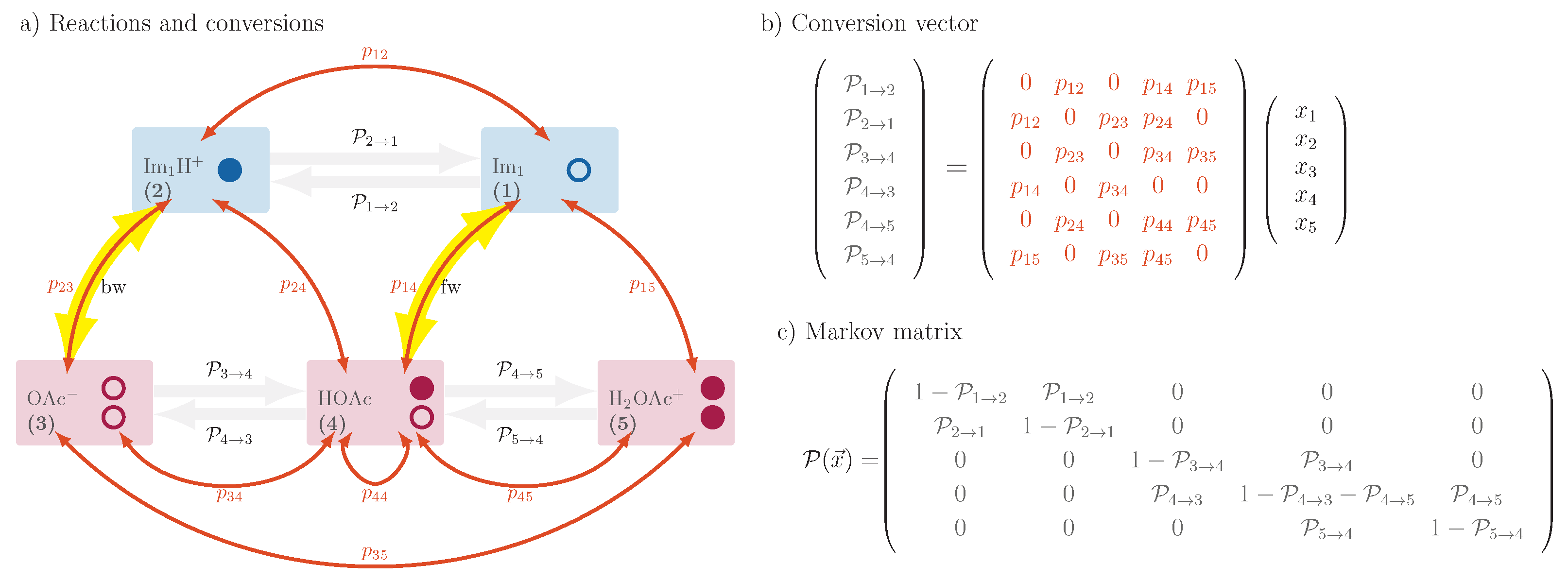
• The reaction with another imidazolium (2) with the probability $p_{12}$;
• The reaction with acetic acid HOAc (4) with probability $p_{14}$;
• The reaction with protonated acetic acid H₂OAc⁺ (5) with probability $p_{15}$.

Since Im₁ cannot react with itself or acetate, the corresponding entries in the first row of the reaction matrix in Figure 14b are zero. Conversions can only take place within the same chemical category (i.e., the same color-coded group) by altering their protonation state without changing the fundamental molecular identity. Once the conversion probabilities ${\mathcal{P}}_{i\to j}$ are determined, they are assembled into a Markov matrix $\mathcal{P}\left(\overrightarrow{x}\right)$, as depicted in Figure 14c. The Markov matrix is formulated as a function of the mole fraction vector $\overrightarrow{x}=(x_1,x_2,\dots x_5)$, which encapsulates the current composition of the system. The evolution of the mole fractions over time is governed by the iterative equation:

$$\overrightarrow{x}\left(t\right)=\overrightarrow{x}(t-1)·\mathcal{P}\left(\overrightarrow{x}\right)$$

(35)

where $\overrightarrow{x}$ is a row vector representing the mole fractions of the species at time t. The iterative application of this equation models the temporal progression of the system and ultimately converges to the equilibrium composition. Fortunately, the set of QM-derived probabilities for the 1-methylimidazolium acetate system delivers a composition close to the experimental composition [86].

Our program, PROTEX [171,172], employs this validated set of probabilities to perform molecular conversions during polarizable MD simulations. At predefined intervals, the simulation is paused, and the latest configuration is analyzed to compute distances between dummy atoms and proton-transfer hydrogens. If the distance between these atoms falls below a specified threshold, an exchange between the dummy and the proton-transfer hydrogen is executed with the corresponding probability $p_{ij}$, as illustrated in Figure 8. Thereafter, the polarizable MD simulation resumes until the next scheduled interruption. During a typical 50 $\mathrm{n}$$\mathrm{s}$ trajectory production, approximately 5000 interruptions are expected, given that the interval between interruptions is generally around 10 $\mathrm{p}$$\mathrm{s}$ [86]. Each interruption involves several hundred proton transfer events. As a result, the reactive system rapidly reaches the equilibrium composition within a few nanoseconds [172], irrespective of the initial state, which may be fully charged, fully neutral, or any intermediate composition. PROTEX offers several notable advantages in terms of file handling and trajectory analysis: The sequence of atoms in the topology file (see Figure 2) remains unchanged during proton transfer events, ensuring that atomic indices remain constant throughout the simulation. This consistency greatly facilitates subsequent trajectory analysis, e.g., visualization in VMD can be performed without requiring any supplementary code. The computational overhead introduced by PROTEX is approximately 10–20% of the total simulation time, depending on the frequency of interruptions. This efficiency enables the investigation of large systems over extended simulation periods, thereby allowing the computation of macroscopic properties like conductivity. However, PROTEX also has certain limitations. Currently, it has been tested exclusively for proton transfer reactions. Although the framework may apply to processes such as CO₂ chemisorption, its use with even larger moieties is restricted by the requirement that each molecule must contain an adequate number of dummy atoms, rendering crosslinking polymer reactions infeasible. Furthermore, the interval for interrupting the polarizable MD simulation is fixed to conserve computational resources. During these intervals, no reactions occur, and while shorter intervals might allow for more frequent reactions, they would incur higher computational costs and might not permit sufficient system relaxation. Adequate relaxation is crucial to ensure that product molecules can diffuse apart; otherwise, the system risks becoming trapped in rapid, reversible exchanges between the same molecular species.

Crosslinking polymer reactions are best conducted using the REACTER module in LAMMPS [176,177,178], as it eliminates the need for dummy atoms and instead directly modifies the molecular topology. Additionally, REACTER allows for continuous reaction events without being constrained by fixed intervals. However, depending on the specific simulation setup, the computational cost of REACTER can be significantly higher, potentially limiting the feasible system size and simulation duration. Furthermore, it should be noted that REACTER has not yet been applied to ILs.

4. Current Limitations in Reactive Molecular Dynamics

There is no universally superior method for investigating chemical reactions in ILs, as each approach presents specific advantages and limitations. AIMD simulations are a natural choice for studying chemical reactivity, as they inherently describe bond formation and dissociation through transient changes in electron density. These simulations primarily focus on elucidating transition states and reaction mechanisms rather than probing bulk properties of the reactive system. AIMD requires minimal empirical knowledge and offers high transferability across different reactive systems, making it particularly suitable for studying fundamental reaction dynamics. Additionally, modifications to reactants, such as the introduction of functional moieties, can be explored without extensive reparameterization.

However, the computational cost associated with AIMD simulations is substantial, imposing severe constraints on both system size and simulation period. Typically, AIMD simulations can accommodate only ∼1000 atoms for approximately 100 $\mathrm{p}$$\mathrm{s}$, as indicated by the blue region in Figure 15. This limitation restricts both the statistical sampling of reaction events and the ability to investigate environmental influences on reactivity. One strategy to extend sampling time is the use of computationally less expensive electronic structure methods to approximate the electronic energy and its gradients [107]. Bodo and co-workers have employed density functional tight binding (DFTB) to describe ILs, assessing its accuracy by comparing results with full ab initio DFT calculations [107].

Another approach to overcoming system size limitations involves hybrid multiscale simulations, where the reactive region is treated quantum mechanically while the surrounding solvent is described by a conventional force field. This hybrid approach extends system sizes beyond those accessible with pure AIMD, as represented by the yellow region in Figure 15. However, the computational bottleneck remains the QM calculations, meaning that the total accessible simulation time does not significantly exceed that of AIMD. To mitigate this limitation, Acevedo and co-workers [118,124,125,126,127,128] adopted a Monte Carlo sampling approach, generating new configurations rather than performing conventional MD. While this enhances the sampling of the reaction space, it precludes the calculation of dynamic properties, as the trajectory does not follow a physical time evolution. Despite the benefits of multiscale, certain drawbacks remain. Typically, the QM region is smaller than in AIMD simulations, often containing only a single reactive site immersed in a solvent environment. This restriction prevents phenomena such as coupled reactions depicted in Figure 14 and consecutive proton hopping, which is essential in many IL-related reaction mechanisms. Furthermore, the macroscopic composition of the liquid is not fully represented in the reactive region, potentially leading to inaccuracies in bulk property predictions. The boundary between the QM and classical regions presents additional challenges, as the electrostatic interactions remain static in the force field region and do not dynamically respond to changes in electron density [199].

To overcome these constraints and enable the simulation of larger, more homogeneous reactive regions, continuous reactive force fields, such as ReaxFF, provide a viable alternative. As illustrated by the green area in Figure 15, ReaxFF allows for extended system sizes and simulation periods, although typically one of these is prioritized. For instance, if system sizes remain comparable to AIMD, the accessible simulation time can reach the nanosecond range [200]. However, ReaxFF exhibits intrinsic limitations. One critical drawback is the lack of explicit charge transfer treatment, which affects the accuracy of ion mobility calculations. Additionally, ReaxFF often necessitates system-specific parameterization, a labor-intensive process that is not easily transferable across different ILs. The parameterization workflow is typically based on static QM calculations, potentially overlooking crucial dynamical effects [55]. Furthermore, due to the need for high numerical stability, the time step in ReaxFF is often reduced to 0.1 fs to 0.25 fs, significantly increasing the computational cost. To enhance the efficiency of ReaxFF and accelerate rare event sampling, biasing techniques such as the bond-boost [194] method can be employed [201]. This approach introduces artificial energy terms to facilitate bond-breaking processes once bond lengths approach transition-state configurations [194]. Additionally, GPU-accelerated implementations of ReaxFF, developed and optimized by Guo and co-workers [202,203], have demonstrated computational speed-ups of nearly two orders of magnitude compared to conventional CPU-based ReaxFF calculations. Despite these improvements, ReaxFF simulations still struggle to accurately reproduce key macroscopic properties such as viscosity and ionic conductivity, which require system sizes of at least 500 ion pairs and simulation times exceeding 20 $\mathrm{n}$$\mathrm{s}$ [112]. Another significant limitation is the lack of explicit long-range electrostatic interactions in standard ReaxFF implementations, which impacts ionic association dynamics and, consequently, fundamental transport properties such as ion diffusion and conductivity.

For simulations aiming to capture macroscopic properties, such as viscosity, conductivity, and nanoscale phase segregation of polar and apolar domains, as well as to model extensive reactive environments that enable consecutive proton hopping, fractional force fields offer a promising alternative. PROTEX simulations incorporate these fractional force fields by periodically interrupting conventional polarizable MD simulations at fixed intervals of usually 10 $\mathrm{p}$$\mathrm{s}$ [171,172]. During conventional trajectory propagation, no chemical reactions occur. Instead, multiple (up to hundreds of) reactions take place simultaneously during these interruptions, leading to instantaneous transitions between reactant and product states. However, this approach precludes a detailed investigation of reaction pathways, as the system does not explicitly follow the potential energy surfaces including the transition state. The probabilities of overcoming the transition states must be determined prior to the simulation, limiting the transferability of the parameters when modifying reactants or products. PROTEX employs a single-topology framework with dummy atoms, allowing for small moiety exchanges between reactant and product states. However, due to this constraint, cross-linking reactions in polymeric ILs cannot be simulated, despite PROTEX’s capability to model system sizes large enough to capture long-range Coulombic interactions. These approximations enable significantly larger system sizes and longer simulation times than any other method discussed, as illustrated by the red area in the top right corner of Figure 15, which has logarithmic size and time scales.

5. Conclusions and Outlook

Over the past two decades, the field of reactive molecular dynamics in ILs has witnessed substantial advancements, as illustrated in Figure 3. AIMD simulations remain the predominant approach due to their versatility in elucidating reaction mechanisms. However, their high computational cost severely limits both system size and simulation duration. Hybrid multiscale methods provide a viable compromise by extending system sizes while preserving chemical accuracy in the reactive region. Despite these advantages, QM/MM simulations are still constrained in their ability to capture large-scale dynamic processes, such as consecutive proton transfers and bulk transport phenomena. Consequently, only a limited number of multiscale studies generate full trajectories, as reflected by the relatively low number of references (indicated by orange dots) in Figure 15. More commonly, multiscale techniques are integrated with Monte Carlo algorithms to explore reaction pathways [118,124,125,126,127,128]. The development of faster computational architectures and more efficient algorithms [204] would enhance the temporal reach of both QM-based methods, further strengthening their applicability.

Reactive force fields, such as ReaxFF, present an alternative framework that enables the simulation of bond formation and cleavage in substantially larger systems over extended timescales. However, these simulations necessitate extensive parameterization, which poses challenges in their generalizability across different ILs. Additionally, ReaxFF struggles to accurately capture long-range electrostatic interactions, thereby limiting its effectiveness in modeling key macroscopic properties such as viscosity and ionic conductivity. While machine learning techniques offer promising avenues for automating the parameterization process [205,206,207,208], the computational expense associated with trajectory production in ReaxFF remains significantly higher than that of conventional MD simulations.

Beyond reactive force fields, machine-learning-based approaches are emerging as powerful tools for both property prediction [209] and MD trajectory generation [210,211,212]. Despite their potential, these methods remain computationally demanding, imposing similar limitations on simulation time and system size as those encountered in ReaxFF. Furthermore, machine-learning-based approaches require vast quantities of high-quality experimental and computational data for effective training, which are currently insufficiently available. Given these constraints, the methods reviewed in this review remain indispensable and should be employed more extensively than they presently are to drive further progress in the field.

A promising recent development is the introduction of fractional force fields, exemplified by the PROTEX [171,172] framework, which offers a novel means of capturing large-scale reactive environments. By intermittently interrupting conventional MD simulations to introduce predefined reaction probabilities, PROTEX facilitates the modeling of extensive reaction networks over nanosecond timescales. This approach enables the investigation of bulk properties such as proton-transfer-enhanced conductivity in ILs, which are otherwise inaccessible using conventional reactive MD techniques. Here as well, machine learning has the potential to refine reaction probabilities, thereby improving predictive accuracy. Expanding the applicability of fractional force fields beyond proton transfer reactions to encompass a broader range of chemical transformations—such as CO₂ chemisorption, electrode passivation, and charge transfer in electrochemical systems—would substantially enhance their utility.

Ultimately, the continued refinement of reactive MD methodologies will be pivotal in advancing our understanding of complex reaction networks in condensed-phase environments. By leveraging the complementary strengths of different computational approaches, future studies can provide a more holistic representation of chemical reactivity, effectively bridging the gap between atomistic simulations and experimentally observed macroscopic properties.

References

1. Reichardt, C.; Welton, T. Solvents and Solvent Effects in Organic Chemistry, 4th ed.; Wiley-VCH: Weinheim, Germany, 2011. [Google Scholar]
2. Hallett, J.P.; Welton, T. Room-Temperature Ionic Liquids: Solvents for Synthesis and Catalysis. 2. Chem. Rev. 2011, 111, 3508–3576. [Google Scholar] [CrossRef] [PubMed]
3. Hubbard, C.D.; Illner, P.; van Eldik, R. Understanding Chemical Reaction Mechanisms in Ionic Liquids: Successes and Challenges. Chem. Soc. Rev. 2011, 40, 272–290. [Google Scholar] [CrossRef]
4. Yoshizawa, M.; Xu, W.; Angell, C.A. Ionic Liquids by Proton Transfer: Vapor Pressure, Conductivity, and the Relevance of ΔpKa from Aqueous Solutions. J. Am. Chem. Soc. 2003, 125, 15411–15419. [Google Scholar] [CrossRef] [PubMed]
5. Belieres, J.P.; Angell, C.A. Protic Ionic Liquids: Preparation, Characterization, and Proton Free Energy Level Representation. J. Phys. Chem. B 2007, 111, 4926–4937. [Google Scholar] [CrossRef] [PubMed]
6. Greaves, T.L.; Drummond, C.J. Protic Ionic Liquids: Properties and Applications. Chem. Rev. 2008, 108, 206–237. [Google Scholar] [CrossRef]
7. Bailey, J.; Byrne, E.L.; Goodrich, P.; Kavanagh, P.; Swadźba-Kwaśny, M. Protic ionic liquids for sustainable uses. Green Chem. 2024, 26, 1092–1131. [Google Scholar] [CrossRef]
8. Fumino, K.; Wulf, A.; Ludwig, R. Hydrogen Bonding in Protic Ionic Liquids: Reminiscent of Water. Angew. Chem. Int. Ed. 2009, 48, 3184–3186. [Google Scholar] [CrossRef]
9. Fumino, K.; Fossog, V.; Stange, P.; Paschek, D.; Hempelmann, R.; Ludwig, R. Controlling the Subtle Energy Balance in Protic Ionic Liquids: Dispersion Forces Compete with Hydrogen Bonds. Angew. Chem. Int. Ed. 2015, 54, 2792–2795. [Google Scholar] [CrossRef]
10. Doi, H.; Song, X.; Minofar, B.; Kanzaki, R.; Takamuku, T.; Umebayashi, Y. A New Proton Conductive Liquid with No Ions: Pseudo-Protic Ionic Liquids. Chem. Eur. J. 2013, 19, 11522–11526. [Google Scholar] [CrossRef]
11. Stoimenovski, J.; Izgorodina, E.I.; MacFarlane, D.R. Ionicity and proton transfer in protic ionic liquids. Phys. Chem. Chem. Phys. 2010, 12, 10341–10347. [Google Scholar] [CrossRef]
12. MacFarlane, D.R.; Pringle, J.M.; Johansson, K.M.; Forsyth, S.A.; Forsyth, M. Lewis base ionic liquids. Chem. Commun. 2006, 1905–1917. [Google Scholar] [CrossRef] [PubMed]
13. Hou, H.Y.; Huang, Y.R.; Wang, S.Z.; Bai, B.F. Preparation and Physicochemical Properties of Imidazolium Acetates and the Conductivities of Their Aqueous and Ethanol Solutions. Acta Phys. Chim. Sin. 2011, 27, 2512–2520. [Google Scholar]
14. Chen, J.; Chen, L.; Lu, Y.; Xu, Y. Physicochemical properties of aqueous solution of 1-methylimidazolium acetate ionic liquid at several temperatures. J. Mol. Liq. 2014, 197, 374–380. [Google Scholar] [CrossRef]
15. Thawarkar, S.; Khupse, N.D.; Shinde, D.R.; Kumar, A. Understanding the behavior of mixtures of protic-aprotic and protic-protic ionic liquids: Conductivity, viscosity, diffusion coefficient and ionicity. J. Mol. Liq. 2019, 276, 986–994. [Google Scholar] [CrossRef]
16. Joerg, F.; Schröder, C. Polarizable molecular dynamics simulations on the conductivity of pure 1-methylimidazolium acetate systems. Phys. Chem. Chem. Phys. 2022, 24, 15245. [Google Scholar] [CrossRef]
17. Joerg, F.; Sutter, J.; van Dam, L.; Kanellopoulos, K.; Hunger, J.; Schröder, C. Comparative analysis of dielectric spectra in protic ionic liquids: Experimental findings and computational molecular decomposition. J. Mol. Liq. 2024, 396, 123834. [Google Scholar] [CrossRef]
18. Overbeck, V.; Ludwig, R. NMR Studies of Protic Ionic Liquids. In Annual Reports on NMR Spectroscopy; Elsevier: Amsterdam, The Netherlands, 2018; Volume 95, pp. 147–190. [Google Scholar]
19. Chen, K.; Wang, Y.; Yao, J.; Li, H. Equilibrium in Protic Ionic Liquids: The Degree of Proton Transfer and Thermodynamic Properties. J. Phys. Chem. B 2018, 122, 309–315. [Google Scholar] [CrossRef]
20. Hasani, M.; Amin, S.A.; Yarger, J.L.; Davidowski, S.K.; Angell, C.A. Proton Transfer and Ionicity: An 15N NMR Study of Pyridine Base Protonation. J. Phys. Chem. B 2019, 123, 1815–1821. [Google Scholar] [CrossRef]
21. Calandra, P.; Caputo, P.; Rossi, C.O.; Kozak, M.; Taube, M.; Pochylski, M.; Gapinski, J. From proton transfer to ionic liquids: How isolated domains of ion pairs grow to form extended network in diphenyl phosphate-bis(2-ethylhexyl) amine mixtures. J. Mol. Liq. 2024, 399, 124402. [Google Scholar] [CrossRef]
22. Hoarfrost, M.L.; Tyagi, M.; Segalman, R.A.; Reimer, J.A. Proton Hopping and Long-Range Transport in the Protic Ionic Liquid [Im][TFSI], Probed by Pulsed-Field Gradient NMR and Quasi-Elastic Neutron Scattering. J. Phys. Chem. B 2012, 116, 8201–8209. [Google Scholar] [CrossRef]
23. Kobrak, M.N.; Nykypanchuk, D.; Jain, A.; Louz, E.; Jarzecki, A.A. Proton Transfer Equilibrium in Pseudoprotic Ionic Liquids: Inferences on Ionic Populations. J. Phys. Chem. B 2025, 129, 1376–1386. [Google Scholar] [CrossRef] [PubMed]
24. Watanabe, H.; Arai, N.; Han, J.; Kawana, Y.; Tsuzuki, S.; Umebayashi, Y. Tools for studying ion solvation and ion pair formation in ionic liquids: Isotopic substitution Raman spectroscopy. Anal. Sci. 2022, 38, 1025–1031. [Google Scholar] [CrossRef] [PubMed]
25. Sun, X.; Cao, B.; Zhou, X.; Liu, S.; Zhu, X.; Fu, H. Theoretical and experimental studies on proton transfer in acetate-based protic ionic liquids. J. Mol. Liq. 2016, 221, 254–261. [Google Scholar] [CrossRef]
26. Mann, S.K.; Brown, S.P.; MacFarlane, D.R. Structure Effects on the Ionicity of Protic Ionic Liquids. ChemPhysChem 2020, 21, 1444–1454. [Google Scholar] [CrossRef]
27. Kanzaki, R.; Uchida, K.; Song, X.; Umebayashi, Y.; Ishiguro, S.I. Acidity and Basicity of Aqueous Mixtures of a Protic Ionic Liquid, Ethylammonium Nitrate. Anal. Sci. 2008, 24, 1347–1349. [Google Scholar] [CrossRef]
28. Kanzaki, R.; Song, X.; Umebayashi, Y.; Ishiguro, S. Thermodynamic Study of the Solvation States of Acid and Base in a Protic Ionic Liquid, Ethylammonium Nitrate, and Its Aqueous Mixtures. Chem. Lett. 2010, 39, 578–579. [Google Scholar] [CrossRef]
29. Song, X.; Kanzaki, R.; Ishiguro, S.; Umebayashi, Y. Physicochemical and Acid-base Properties of a Series of 2-Hydroxyethylammonium-based Protic Ionic Liquids. Anal. Sci. 2012, 28, 469–474. [Google Scholar] [CrossRef]
30. Qian, W.; Xu, Y.; Zhu, H.; Yu, C. Properties of pure 1-methylimidazolium acetate ionic liquid and its binary mixtures with alcohols. J. Chem. Thermodyn. 2012, 49, 87–94. [Google Scholar] [CrossRef]
31. Ingenmey, J.; Gehrke, S.; Kirchner, B. How to Harvest Grotthuss Diffusion in Protic Ionic Liquid Electrolyte Systems. ChemSusChem 2018, 11, 1900–1910. [Google Scholar] [CrossRef]
32. Marx, D. Proton Transfer 200 Years after von Grotthuss: Insights from Ab Initio Simulations. ChemPhysChem 2006, 7, 1848–1870. [Google Scholar] [CrossRef]
33. Hayes, R.; Warr, G.G.; Atkin, R. Structure and Nanostructure in Ionic Liquids. Chem. Rev. 2015, 115, 6357–6426. [Google Scholar] [PubMed]
34. Anouti, M.; Jacquemin, J.; Porion, P. Transport Properties Investigation of Aqueous Protic Ionic Liquid Solutions through Conductivity, Viscosity, and NMR Self-Diffusion Measurements. J. Phys. Chem. B 2012, 116, 4228–4238. [Google Scholar] [CrossRef] [PubMed]
35. Bodo, E. Perspectives in the Computational Modeling of New Generation, Biocompatible Ionic Liquids. J. Phys. Chem. B 2022, 126, 3–13. [Google Scholar] [CrossRef] [PubMed]
36. Kanzaki, R.; Kodamatani, H.; Tomiyasu, T.; Watanabe, H.; Umebayashi, Y. A pH Scale for the Protic Ionic Liquid Ethylammonium Nitrate. Angew. Chem. Int. Ed. 2016, 55, 6266–6269. [Google Scholar] [CrossRef]
37. Abbott, A.P.; Alabdullah, S.S.M.; Al-Murshedia, A.Y.M.; Ryder, K.S. Brønsted acidity in deep eutectic solvents and ionic liquids. Faraday Discuss. 2018, 206, 365–377. [Google Scholar] [CrossRef]
38. Wang, C.; Luo, X.; Zhu, X.; Cui, G.; Jiang, D.E.; Deng, D.; Li, H.; Dai, S. The strategies for improving carbon dioxide chemisorption by functionalized ionic liquids. RSC Adv. 2013, 3, 15518–15527. [Google Scholar] [CrossRef]
39. Sheridan, Q.R.; Schneider, W.F.; Maginn, E.J. Role of Molecular Modeling in the Development of CO2-Reactive Ionic Liquids. Chem. Rev. 2018, 118, 5242–5260. [Google Scholar] [CrossRef]
40. Elmobarak, W.F.; Almomani, F.; Tawalbeh, M.; Al-Othman, A.; Martis, R.; Rasool, K. Current status of CO2 capture with ionic liquids: Development and progress. Fuel 2023, 344, 128102. [Google Scholar] [CrossRef]
41. Bates, E.D.; Mayton, R.D.; Ntai, I.; Davis, J. CO2 capture by a task-specific ionic liquid. J. Am. Chem. Soc. 2002, 124, 926–927. [Google Scholar] [CrossRef]
42. Gurkan, B.; Goodrich, B.F.; Mindrup, E.M.; Ficke, L.E.; Massel, M.; Seo, S.; Senftle, T.P.; Wu, H.; Glaser, M.F.; Shah, J.K.; et al. Molecular Design of High Capacity, Low Viscosity, Chemically Tunable Ionic Liquids for CO2 Capture. J. Phys. Chem. Lett. 2010, 1, 3494–3499. [Google Scholar] [CrossRef]
43. Lepre, L.F.; Szala-Bilnik, J.; Pison, L.; Traïkia, M.; Padua, A.A.H.; Ando, R.A.; Costa Gomes, M.F. Can the tricyanomethanide anion improve CO2 absorption by acetate-based ionic liquids? Phys. Chem. Chem. Phys. 2017, 19, 12431–12440. [Google Scholar] [CrossRef] [PubMed]
44. Gurau, G.; Rodríguez, H.; Kelley, S.P.; Janiczek, P.; Kalb, R.S.; Rogers, R.D. Demonstration of Chemisorption of Carbon Dioxide in 1,3-Dialkylimidazolium Acetate Ionic Liquids. Angew. Chem. Int. Ed. 2011, 50, 12024–12026. [Google Scholar] [CrossRef] [PubMed]
45. Blath, J.; Deubler, N.; Hirth, T.; Schiestel, T. Chemisorption of carbon dioxide in imidazolium based ionic liquids with carboxylic anions. Chem. Eng. J. 2012, 181–182, 152–158. [Google Scholar] [CrossRef]
46. Karadas, F.; Köz, B.; Jacquemin, J.; Deniz, E.; Rooney, D.; Thompson, J.; Yavuz, C.T.; Khraisheh, M.; Aparicio, S.; Atihan, M. High-pressure CO2 absorption studies on imidazolium-based ionic liquids: Experimental and simulation approaches. Fluid Phase Equil. 2013, 351, 74–86. [Google Scholar] [CrossRef]
47. Cao, B.; Yan, W.; Wang, J.; Ding, H.; Yu, Y. Absorption of CO2 with supported imidazolium-based ionic liquid membranes. J. Chem. Technol. Biotechnol. 2015, 90, 1537–1544. [Google Scholar] [CrossRef]
48. Wang, C.; Luo, H.; Luo, X.; Li, H.; Dai, S. Equimolar CO2 capture by imidazolium-based ionic liquids and superbase systems. Green Chem. 2010, 12, 2019–2023. [Google Scholar] [CrossRef]
49. Peng, Y.; Szeto, K.C.; Santini, C.; Daniele, S. Study of the Parameters Impacting the Photocatalytic Reduction of Carbon Dioxide in Ionic Liquids. ChemPhotoChem 2021, 5, 721–726. [Google Scholar] [CrossRef]
50. Peng, Y.; Szeto, K.C.; Santini, C.; Daniele, S. Ionic Liquids as homogeneous photocatalyst for CO2 reduction in protic solvents. Chem. Eng. J. Adv. 2022, 12, 100379. [Google Scholar] [CrossRef]
51. Suo, X.; Fu, Y.; Do-Thanh, C.L.; Qiu, L.Q.; Jiang, D.; Mahurin, S.M.; Yang, Z.; Dai, S. CO2 Chemisorption Behavior in Conjugated Carbanion-Derived Ionic Liquids via Carboxylic Acid Formation. J. Am. Chem. Soc. 2022, 144, 21658–21663. [Google Scholar] [CrossRef]
52. Arduengo, A.J., III; Harlow, R.L.; Kline, M. A Stable Crystalline Carbene. J. Am. Chem. Soc. 1991, 113, 361–363. [Google Scholar] [CrossRef]
53. Cabacço, M.I.; Besnard, M.; Danten, Y.; Coutinho, J.A.P. Carbon Dioxide in 1-Butyl-3-methylimidazolium Acetate. I. UnusualSolubility Investigated by Raman Spectroscopy and DFT Calculations. J. Phys. Chem. A 2012, 116, 1605–1620. [Google Scholar] [CrossRef] [PubMed]
54. Canongia Lopes, J.N.A.; Pádua, A.A.H. Nanostructural Organization in Ionic Liquids. J. Phys. Chem. B 2006, 110, 3330–3335. [Google Scholar] [CrossRef] [PubMed]
55. Farah, K.; Müller-Plathe, F.; Böhm, M.C. Classical Reactive Molecular Dynamics Implementations: State of the Art. ChemPhysChem 2012, 13, 1127–1151. [Google Scholar] [CrossRef]
56. Bedrov, D.; Piquemal, J.P.; Borodin, O.; MacKerell, A.; Roux, B.; Schröder, C. Molecular Dynamics Simulations of Ionic Liquids and Electrolytes Using Polarizable Force Fields. Chem. Rev. 2019, 119, 7940–7995. [Google Scholar] [CrossRef]
57. van Gunsteren, W.F.; Oostenbrink, C. Methods for Classical-Mechanical Molecular Simulation in Chemistry: Achievements, Limitations, Perspectives. J. Chem. Inf. Model. 2024, 64, 6281–6304. [Google Scholar] [CrossRef]
58. Hunt, P.A. The simulation of imidazolium-based ionic liquids. Mol. Sim. 2006, 32, 1–10. [Google Scholar] [CrossRef]
59. Maginn, E.J. Molecular simulation of ionic liquids: Current status and future opportunities. J. Phys. Condens. Matter 2009, 21, 373101. [Google Scholar] [CrossRef]
60. Liu, T.; Panwar, P.; Khajeh, A.; Rahman, M.H.; Menezes, P.L.; Martini, A. Review of Molecular Dynamics Simulations of Phosphonium Ionic Liquid Lubricants. Tribol. Lett. 2022, 70, 44. [Google Scholar] [CrossRef]
61. Humphrey, W.; Dalke, A.; Schulten, K. VMD—Visual Molecular Dynamics. J. Mol. Graph. 1996, 14, 33–38. [Google Scholar] [CrossRef]
62. Gowers, R.J.; Linke, M.; Barnoud, J.; Reddy, T.J.E.; Melo, M.N.; Seyler, S.L.; Dotson, D.L.; Domanski, J.; Buchoux, S.; Kenney, I.M.; et al. MDAnalysis: A python package for the rapid analysis of molecular dynamics simulations. In Proceedings of the 15th Python in Science Conference, Austin, TX, USA, 11–17 July 2016; Benthall, S., Rostrup, S., Eds.; Los Alamos National Laboratory: Los Alamos, NM, USA, 2016. [Google Scholar]
63. McCann, B.W.; Acevedo, O. Pairwise Alternatives to Ewald Summation for Calculating Long-Range Electrostatics in Ionic Liquids. J. Chem. Theory Comput. 2013, 9, 944–950. [Google Scholar] [CrossRef]
64. Hünenberger, P.H.; McCammon, J.A. Ewald artifacts in computer simulations of ionic solvation and ion–ion interaction: A continuum electrostatics study. J. Chem. Phys. 1999, 110, 1856–1872. [Google Scholar] [CrossRef]
65. Wells, B.A.; Chaffee, A.L. Ewald Summation for Molecular Simulations. J. Chem. Theory Comput. 2015, 11, 3684–3695. [Google Scholar] [CrossRef] [PubMed]
66. Hammonds, K.D.; Heyes, D.M. Optimization of the Ewald method for calculating Coulomb interactions in molecular simulations. J. Chem. Phys. 2022, 157, 074108. [Google Scholar] [CrossRef] [PubMed]
67. Aguado, A.; Madden, P.A. Ewald summation of electrostatic multipole interactions up to the quadrupolar level. J. Chem. Phys. 2003, 119, 7471–7483. [Google Scholar] [CrossRef]
68. Lamichhane, M.; Newman, K.E.; Gezelter, J.D. Real space electrostatics for multipoles. II. Comparisons with the Ewald sum. J. Chem. Phys. 2014, 141, 134110. [Google Scholar] [CrossRef]
69. Hanke, C.G.; Price, S.L.; Lynden-Bell, R.M. termolecular potentials for simulations of liquid imidazolium salts. Mol. Phys. 2001, 99, 801–809. [Google Scholar] [CrossRef]
70. Del Pópolo, M.G.; Kohanoff, J.; Lynden-Bell, R.M. Solvation structure and transport of acidic protons in ionic liquids: A first-principles simulation study. J. Phys. Chem. B 2006, 110, 8798–8803. [Google Scholar] [CrossRef]
71. Canongia Lopes, J.N.; Deschamps, J.; Pádua, A.A.H. Modeling Ionic Liquids Using a Systematic All-Atom Force Field. J. Phys. Chem. B 2004, 108, 2038–2047. [Google Scholar] [CrossRef]
72. Schröder, C. Comparing reduced partial charge models with polarizable simulations of ionic liquids. Phys. Chem. Chem. Phys. 2012, 14, 3089–3102. [Google Scholar] [CrossRef]
73. Morrow, T.I.; Maginn, E.J. Molecular Dynamics Study of the Ionic Liquid 1-n-Butyl-3-methylimidazolium Hexafluorophosphat. J. Phys. Chem. 2002, 106, 12807–12813. [Google Scholar] [CrossRef]
74. Sappl, M.; Gross, S.; Hugger, P.T.; D’Alessio, P.; Palka, M.; Felix Fritz, S.; Spange, S.; Schröder, C. Decomposition, interpretation and prediction of various ionic liquid solvation parameters: Kamlet-Taft, Catalán and Reichardt’s ETN. J. Mol. Liq. 2024, 417, 126646. [Google Scholar] [CrossRef]
75. Dommert, F.; Wendler, K.; Berger, R.; Delle Site, L.; Holm, C. Force Fields for Studying the Structure and Dynamics of Ionic Liquids: A Critical Review of Recent Developments. ChemPhysChem 2012, 13, 1625–1637. [Google Scholar] [CrossRef] [PubMed]
76. McDaniel, J.G.; Yethiraj, A. The Influence of Electronic Polarization on the Structure of Ionic Liquids. J. Phys. Chem. Lett. 2018, 9, 4765–4770. [Google Scholar] [CrossRef] [PubMed]
77. Méndez-Morales, T.; Carrete, J.; Cabeza, Ó; Russina, O.; Triolo, A.; Gallego, L.J.; Varela, L.M. Solvation of Lithium Salts in Protic Ionic Liquids: A Molecular Dynamics Study. J. Phys. Chem. B 2014, 118, 761–770. [Google Scholar] [CrossRef]
78. Paschek, D.; Golub, B.; Ludwig, R. Hydrogen bonding in a mixture of protic ionic liquids: A molecular dynamics simulation study. Phys. Chem. Chem. Phys. 2015, 17, 8431–8440. [Google Scholar] [CrossRef]
79. Gontrani, L.; Bodo, E.; Triolo, A.; Leonelli, F.; D’Angelo, P.; Migliorati, V.; Caminiti, R. The Interpretation of Diffraction Patterns of Two Prototypical ProticIonic Liquids: A Challenging Task for Classical Molecular DynamicsSimulations. J. Phys. Chem. B 2012, 116, 13024–13032. [Google Scholar] [CrossRef]
80. Docampo-Álvarez, B.; Gómez-González, V.; Méndez-Morales, T.; Rodríguez, J.R.; Cabeza, O.; Turmine, M.; Gallegoa, L.J.; Varela, L.M. The effect of alkyl chain length on the structure and thermodynamics of protic–aprotic ionic liquid mixtures: A molecular dynamics study. Phys. Chem. Chem. Phys. 2018, 20, 9939–9949. [Google Scholar] [CrossRef]
81. Gómez-González, V.; Docampo-Álvarez, B.; Otero-Mato, J.M.; Cabeza, O.; Gallego, L.J.; Varela, L.M. Molecular dynamics simulations of the structure of mixtures of protic ionic liquids and monovalent and divalent salts at the electrochemical interface. Phys. Chem. Chem. Phys. 2018, 20, 12767–12776. [Google Scholar] [CrossRef]
82. Borodin, O. Polarizable Force Field Development and Molecular Dynamics Simulations of Ionic Liquids. J. Phys. Chem. B 2009, 113, 11463–11478. [Google Scholar] [CrossRef]
83. Goloviznina, K.; Gong, Z.; Costa Gomes, M.F.; Pádua, A.A.H. Extension of the CL&Pol Polarizable Force Field to Electrolytes, Protic Ionic Liquids, and Deep Eutectic Solvents. J. Chem. Theory Comput. 2021, 17, 1606–1617. [Google Scholar]
84. Goloviznina, K.; Gong, Z.; Pádua, A.A.H. The CL&Pol polarizable force field for the simulation of ionic liquids and eutectic solvents. WIREs Comput. Mol. Sci. 2021, 12, e1572. [Google Scholar]
85. Nasrabadi, A.T.; Gelb, L.D. How proton tranfer equilibria influence ionic liquid properties: Molecular simulations of alkylammonium acetates. J. Phys. Chem. B 2018, 122, 5961–5971. [Google Scholar] [CrossRef] [PubMed]
86. Jacobi, R.; Joerg, F.; Schröder, C. Emulating proton transfer reactions in the pseudo-protic ionic liquid 1-methylimidazolium acetate. Phys. Chem. Chem. Phys. 2022, 24, 9277–9285. [Google Scholar] [CrossRef] [PubMed]
87. Ponder, J.W.; Wu, C.; Ren, P.; Pande, V.S.; Chodera, J.D.; Schnieders, M.J.; Haque, I.; Mobley, D.L.; Lambrecht, D.S.; DiStasio, R.A., Jr.; et al. Current Status of the AMOEBA Polarizable Force Field. J. Phys. Chem. B 2010, 114, 2549–2564. [Google Scholar] [CrossRef]
88. Starovoytov, O.N.; Torabifard, H.; Cisneros, G.A. Development of AMOEBA Force Field for 1,3-Dimethylimidazolium Based Ionic Liquids. J. Phys. Chem. B 2014, 118, 7156–7166. [Google Scholar] [CrossRef]
89. Vázquez-Montelongo, E.A.; Vázquez-Cervantes, J.E.; Cisneros, G.A. Current Status of AMOEBA–IL: A Multipolar/Polarizable Force Field for Ionic Liquids. Int. J. Mol. Sci. 2020, 21, 697. [Google Scholar] [CrossRef]
90. Szabadi, A.; Schröder, C. Recent developments in polarizable molecular dynamics simulations of electrolyte solutions. J. Comput. Biophys. Chem. 2021, 21, 415–429. [Google Scholar] [CrossRef]
91. Bernardes, C.E.S.; Shimizu, K.; Lopes, J.N.C.; Marquetand, P.; Heid, E.; Steinhauser, O.; Schröder, C. Additive polarizabilities in ionic liquids. Phys. Chem. Chem. Phys. 2016, 18, 1665–1670. [Google Scholar] [CrossRef]
92. Philippi, F.; Quinten, A.; Rauber, D.; Springborg, M.; Hempelmann, R. Density Functional Theory Descriptors for Ionic Liquids and theIntroduction of a Coulomb Correction. J. Phys. Chem. A 2019, 123, 4188–4200. [Google Scholar] [CrossRef]
93. Philippi, F.; Goloviznina, K.; Gong, Z.; Gehrke, S.; Kirchner, B.; Pádua, A.A.H.; Hunt, P.A. Charge transfer and polarisability in ionic liquids: A case study. Phys. Chem. Chem. Phys. 2022, 24, 3144–3162. [Google Scholar] [CrossRef]
94. Olano, L.R.; Rick, S.W. Fluctuating Charge Normal Modes: An Algorithm forImplementing Molecular Dynamics Simulations withPolarizable Potentials. J. Comput. Chem. 2005, 26, 699–707. [Google Scholar] [CrossRef]
95. Patel, S.; Brooks, C.L., III. Fluctuating Charge Force Fields: Recent Developments and Applications From Small Molecules to Macromolecular Biological Systems. Mol. Simul. 2006, 32, 231–249. [Google Scholar] [CrossRef]
96. Wendler, K.; Dommert, F.; Zhao, Y.Y.; Berger, R.; Holm, C.; Delle Site, L. Ionic liquids studied across different scales: A computational perspective. Faraday Discuss. 2012, 154, 111–132. [Google Scholar] [CrossRef] [PubMed]
97. Schröder, C.; Lyons, A.; Rick, S.W. Polarizable MD simulations of ionic liquids: How does additional charge transfer change the dynamics. Phys. Chem. Chem. Phys. 2020, 22, 467–477. [Google Scholar] [CrossRef] [PubMed]
98. Heinz, H.; Vaia, R.A.; Koerner, H.; Farmer, B.L. Photoisomerization of azobenzene grafted to layered silicates: Simulation and experimental challenges. Chem. Mater. 2008, 20, 6444–6456. [Google Scholar] [CrossRef]
99. Tian, Z.; Wen, J.; Ma, J. Dynamic simulations of stimuli-responsive swithcing of azobenzene derivatives in self-assembled monolayers: Reactive rotation potential and switching functions. Mol. Simul. 2015, 41, 28–42. [Google Scholar] [CrossRef]
100. Del Pópolo, M.G.; Lynden-Bell, R.M.; Kohanoff, J. Ab Initio Molecular Dynamics Simulation of a Room Temperature Ionic Liquid. J. Phys. Chem. B 2005, 109, 5895–5902. [Google Scholar] [CrossRef]
101. Hohenberg, P.; Kohn, W. Inhomogeneous Electron Gas. Phys. Rev. 1964, 136, B864–B871. [Google Scholar] [CrossRef]
102. Kohn, W.; Sham, L.J. Self-Consistent Equations Including Exchange and Correlation Effects. Phys. Rev. 1965, 140, A1133–A1138. [Google Scholar] [CrossRef]
103. Le Donne, A.; Adenusi, H.; Procelli, F.; Bodo, E. Structural Features of Cholinium Based Protic Ionic Liquids through Molecular Dynamics. J. Phys. Chem. B 2019, 123, 5568–5576. [Google Scholar] [CrossRef]
104. Kirchner, B.; Seitsonen, A.P. Ionic Liquids from Car-Parrinello Simulations. 2. Structural Diffusion Leading to Large Anions in Chloraluminate Ionic Liquids. Inorg. Chem. 2007, 46, 2751–2754. [Google Scholar] [CrossRef] [PubMed]
105. Salanne, M.; Siqueira, L.J.A.; Seitsonen, A.P.; Madden, P.A.; Kirchner, B. From molten salts to room temperature ionic liquids: Simulation studies on chloroaluminate systems. Faraday Discuss. 2012, 154, 171–188. [Google Scholar] [CrossRef] [PubMed]
106. Campetella, M.; Montagna, M.; Gontrani, L.; Bodo, E. Unexpected proton mobility in the bulk phase of cholinium-based ionic liquids: New insights from theoretical calculations. Phys. Chem. Chem. Phys. 2017, 19, 11869. [Google Scholar] [CrossRef]
107. Adenusi, H.; Le Donne, A.; Porcelli, F.; Bodo, E. Ab Initio Molecular Dynamics Study of Phospho-Amino Acid-Based Ionic Liquids: Formation of Zwitterionic Anions in the Presence of Acidic Side Chains. J. Phys. Chem. B 2020, 124, 1955–1964. [Google Scholar] [CrossRef]
108. Brehm, M.; Weber, H.; Pensado, A.S.; Stark, A.; Kirchner, B. Proton transfer and polarity changes in ionic liquid–water mixtures: A perspective on hydrogen bonds from ab initio molecular dynamics at the example of 1-ethyl-3-methylimidazolium acetate–water mixtures: Part 1. Phys. Chem. Chem. Phys. 2012, 14, 5030–5044. [Google Scholar] [CrossRef]
109. Hollóczki, O.; Gerhard, D.; Massone, K.; Szarvas, L.; Németh, B.; Veszprémi, T.; Nyulászi, L. Carbenes in ionic liquids. New J. Chem. 2010, 34, 3004–3009. [Google Scholar] [CrossRef]
110. Thomas, M.; Brehm, M.; Hollóczki, O.; Kirchner, B. How Can a Carbene be Active in an Ionic Liquid? Chem. Eur. J. 2014, 20, 1622–1629. [Google Scholar] [CrossRef]
111. Hollóczki, O.; Firaha, D.S.; Friedrich, J.; Brehm, M.; Cybik, R.; Wild, M.; Stark, A.; Kirchner, B. Carbene Formation in Ionic Liquids: Spontaneous, Induced, or Prohibited? J. Phys. Chem. B 2013, 117, 5898–5907. [Google Scholar] [CrossRef]
112. Gabl, S.; Schröder, C.; Steinhauser, O. Computational studies of ionic liquids: Size does matter and time too. J. Chem. Phys. 2012, 137, 094501. [Google Scholar] [CrossRef]
113. Gray-Weale, A. Correlations in the Structure and Dynamics of Ionic Liquids. Aust. J. Chem. 2009, 62, 288–297. [Google Scholar] [CrossRef]
114. Bowron, D.T.; D’Agostino, C.; Gladden, L.F.; Hardacre, C.; Holbrey, J.D.; Lagunas, M.C.; McGregor, J.; Mantle, M.D.; Mullan, C.L.; Youngs, T.G.A. Structure and Dynamics of 1-Ethyl-3-methylimidazolium Acetate via Molecular Dynamicsand Neutron Diffraction. J. Phys. Chem. B 2010, 114, 7760–7768. [Google Scholar] [CrossRef] [PubMed]
115. Sánchez, M.L.; Corchado, J.C.; Martín, M.E.; Galván, I.F.; Barata-Morgado, R.; Aguilar, M.A. A New QM/MM Method Oriented to the Study of Ionic Liquids. J. Comput. Chem. 2015, 36, 1893–1901. [Google Scholar] [CrossRef] [PubMed]
116. Seduraman, A.; Klähn, M.; Wu, P. Characterization of nano-domains in ionic liquids with molecular simulations. Calphad 2009, 33, 605–613. [Google Scholar] [CrossRef]
117. Chiappe, C.; Pomelli, C.S. Computational Studies on Organic Reactivity in Ionic Liquids. Phys. Chem. Chem. Phys. 2013, 15, 412–423. [Google Scholar] [CrossRef]
118. Acevedo, O. Simulating chemical reactions in ionic liquids using QM/MM methodology. J. Phys. Chem. A 2014, 118, 11653–11666. [Google Scholar] [CrossRef]
119. Vázquez-Montelongo, E.A.; Vázquez-Cervantes, J.E.; Cisneros, G.A. Polarizable ab initio QM/MM Study of the Reaction Mechanism of N-tert-Butyloxycarbonylation of Aniline in [EMIm][BF4]. Molecules 2018, 23, 2830. [Google Scholar] [CrossRef]
120. Bakowies, D.; Thiel, W. Hybrid Models for Combined Quantum Mechanical and Molecular Mechanical Approaches. J. Phys. Chem. 1996, 100, 10580–10594. [Google Scholar] [CrossRef]
121. Zhang, Y.; Lin, H. Flexible-boundary QM/MM calculations: II. Partial charge transfer across the QM/MM boundary that passes through a covalent bond. Theor. Chem. Acc. 2010, 126, 315–322. [Google Scholar] [CrossRef]
122. Shen, Z.; Glover, W.J. Flexible boundary layer using exchange for embedding theories. I. Theory and implementation. J. Chem. Phys. 2021, 155, 224112. [Google Scholar] [CrossRef]
123. Vreven, T.; Morokuma, K. Chapter 3: Hybrid methods: ONIOM (QM:MM) and QM/MM. Annu. Rep. Comput. Chem. 2006, 2, 35–51. [Google Scholar]
124. Acevedo, O.; Jorgensen, W.L. Advances in Quantum and Molecular Mechanical (QM/MM) Simulations for Organic and Enzymatic Reactions. Acc. Chem. Res. 2010, 43, 142–151. [Google Scholar] [CrossRef] [PubMed]
125. Acevedo, O.; Jorgensen, W.L. Quantum and Molecular Mechanical (QM/MM) Monte Carlo Techniques for Modeling Condensed-Phase Reactions. Wiley Interdiscip. Rev. Comput. Mol. Sci. 2014, 4, 422–435. [Google Scholar] [CrossRef] [PubMed]
126. Allen, C.; McCann, B.W.; Acevedo, O. Ionic Liquid Effects on Nucleophilic Aromatic Substitution Reactions from QM/MM Simulations. J. Phys. Chem. B 2015, 119, 743–752. [Google Scholar] [CrossRef] [PubMed]
127. Allen, C.; Sambasivarao, S.V.; Acevedo, O. An Ionic Liquid Dependent Mechanism for Base Catalyzed B-Elimination Reactions from QM/MM Simulations. J. Am. Chem. Soc. 2013, 135, 1065–1072. [Google Scholar] [CrossRef]
128. Acevedo, O.; Jorgensen, W.L.; Evanseck, J.D. Elucidation of Rate Variations for a Diels-Alder Reaction in Ionic Liquids from QM/MM Simulations. J. Chem. Theory Comput. 2007, 3, 132–138. [Google Scholar] [CrossRef]
129. Chen, Y.; Roux, B. Constant-pH Hybrid Nonequilibrium Molecular Dynamics-Monte Carlo Simulation Method. J. Chem. Theory Comput. 2015, 11, 3919–3931. [Google Scholar] [CrossRef]
130. Warshel, A.; Weiss, R.M. An Empirical Valence Bond Approach for Comparing Reactions in Solutions and in Enzymes. J. Am. Chem. Soc. 1980, 102, 6218–6226. [Google Scholar] [CrossRef]
131. Jensen, F.; Norrby, P.O. Transition states from empirical force fields. Theor. Chem. Acc. 2003, 109, 1–7. [Google Scholar]
132. Chang, Y.-T.; Minichino, C.; Miller, W.H. Classical trajectory studies of the molecular dissociation dynamics of formaldehyde: H2CO → H2 + CO. J. Chem. Phys. 1992, 96, 4341–4355. [Google Scholar] [CrossRef]
133. Kim, Y.; Corchado, J.C.; Villa, J.; Xing, J.; Truhlar, D.G. Multiconfiguration molecular mechanics algorithm for potential energy surfaces of chemical reactions. J. Chem. Phys. 2000, 112, 2718–2735. [Google Scholar] [CrossRef]
134. Sonnenberg, J.L.; Wong, K.F.; Voth, G.A.; Schlegel, H.B. Distributed Gaussian Valence Bond Surface Derived from Ab Initio Calculations. J. Chem. Theory Comput. 2009, 5, 949–961. [Google Scholar] [CrossRef] [PubMed]
135. Åqvist, J.; Warshel, A. Simulation of Enzyme Reactions Using Valence Bond Force Fields and Other Hybrid Quantum/Classical Approaches. Chem. Rev. 1993, 93, 2523–2544. [Google Scholar] [CrossRef]
136. Hinsen, K.; Roux, B. Potential of mean force and reaction rates for proton transfer in acetylacetone. J. Chem. Phys. 1997, 106, 3567–3577. [Google Scholar] [CrossRef]
137. Nagaoka, M.; Okuyama-Yoshida, N.; Yamabe, T. Origin of the Transition State on the Free Energy Surface: Intramolecular Proton Transfer Reaction of Glycine in Aqueous Solution. J. Phys. Chem. A 1998, 102, 8202–8208. [Google Scholar] [CrossRef]
138. Okuyama-Yoshida, N.; Nagaoka, M.; Yamabe, T. Potential Energy Function for Intramolecular Proton Transfer Reaction of Glycine in Aqueous Solution. J. Phys. Chem. A 1998, 102, 285–292. [Google Scholar] [CrossRef]
139. Luzkov, V.B. Empirical valence bond study of radical reactions: Hydrogen atom transfer in peroxidation of phenol. Chem. Phys. Lett. 2001, 345, 345–352. [Google Scholar] [CrossRef]
140. Warshel, A. Dynamics of Reactions in Polar Solvents. Semiclassical Trajectory Studies of Electron-Transfer and Proton-Transfer Reactions. J. Phys. Chem. 1982, 86, 2218–2224. [Google Scholar] [CrossRef]
141. Vendrell, O.; Moreno, M.; Lluch, J.M.; Hammes-Schiffer, S. Molecular Dynamics of Excited State Intramolecular Proton Transfer: 2-(2’-Hydroxylphenyl)-4-methyloxazole in Gas Phase, Solution, and Protein Environments. J. Phys. Chem. B 2004, 108, 6616–6623. [Google Scholar] [CrossRef]
142. Voth, G.A. Computer Simulation of Proton Solvation and Transport in Aqueous and Biomolecular Systems. Acc. Chem. Res. 2006, 39, 143–150. [Google Scholar] [CrossRef]
143. Romero, M.; Kushnir, J.S.; Mochi, B.; Velez, C.; Acevedo, O. Monte Carlo QM/MM simulation studies of the Cannizzaro reaction in ionic liquids for improved biofuel production. J. Chem. Phys. 2024, 161, 084117. [Google Scholar] [CrossRef]
144. Schmitt, U.W.; Voth, G.A. Multistate Empirical Valence Bond Model for Proton Transport in Water. J. Phys. Chem. B 1998, 102, 5547–5551. [Google Scholar] [CrossRef]
145. Schmitt, U.W.; Voth, G.A. The computer simulation of proton transport in water. J. Chem. Phys. 1999, 111, 9361–9381. [Google Scholar] [CrossRef]
146. Day, T.J.F.; Soudackov, A.V.; Čuma, M.; Schmitt, U.W.; Voth, G.A. A second generation multistate empirical valence bond model for proton transport in aqueous systems. J. Chem. Phys. 2002, 117, 5839–5849. [Google Scholar] [CrossRef]
147. Wu, Y.; Chen, H.; Wang, F.; Paesani, F.; Voth, G.A. An Improved Multistate Empirical Valence Bond Model for Aqueous Proton Solvation and Transport. J. Phys. Chem. B 2008, 112, 467–482. [Google Scholar] [CrossRef]
148. Chen, H.; Liu, P.; Voth, G.A. Efficient Multistate Reactive Molecular Dynamics Approach Based on Short-Range Effective Potentials. J. Chem. Theory Comput. 2010, 6, 3039–3047. [Google Scholar] [CrossRef]
149. Čuma, M.; Schmitt, U.W.; Voth, G.A. A multi-state empirical valence bond model for acid-base chemistry in aqueous solution. Chem. Phys. 2000, 258, 187–199. [Google Scholar] [CrossRef]
150. Patil, A.B.; Bhanage, B.M. Modern ab initio valence bond theory calculations reveal charge shift bonding in protic ionic liquids. Phys. Chem. Chem. Phys. 2016, 18, 15783–15790. [Google Scholar] [CrossRef]
151. Patila, A.B.; Bhanage, B.M. Brønsted acidity of protic ionic liquids: A modern ab initio valence bond theory perspective. Phys. Chem. Chem. Phys. 2016, 18, 26020–26025. [Google Scholar] [CrossRef]
152. Brenner, D.W.; Shenderova, O.A.; Harrison, J.A.; Stuart, S.J.; Ni, B.; Sinnott, S.B. A second-generation reactive empirical bond order (REBO) potential energy expression for hydrocarbons. J. Phys. Condens. Matter 2002, 14, 783–802. [Google Scholar] [CrossRef]
153. Xiao, Y.; Dong, W.; Busnengo, H.F. Reactive force fields for surface chemical reactions: A case study with hydrogen dissociation on Pd surfaces. J. Chem. Phys. 2010, 132, 014704. [Google Scholar] [CrossRef]
154. Tersoff, J. New empirical approach for the structure and energy of covalent systems. Phys. Rev. B 1988, 37, 6991–7000. [Google Scholar] [CrossRef] [PubMed]
155. Stuart, S.J.; Tutein, A.B.; Harrison, J.A. A reactive potential for hydrocarbons with intermolecular interactions. J. Chem. Phys. 2000, 112, 6472–6486. [Google Scholar] [CrossRef]
156. Ilyin, D.V.; Goddard, W.A.; Oppenheim, J.J.; Cheng, T. First-principles–based reaction kinetics from reactive molecular dynamics simulations: Application to hydrogen peroxide decomposition. Proc. Natl. Acad. Sci. USA 2019, 116, 18202–18208. [Google Scholar] [CrossRef]
157. Majd Sayed Ahmad, E.M.K.; Giusti, A. A Reactive Molecular Dynamics Investigation of Nanoparticle Interactions in Hydrocarbon Combustion. Combust. Sci. Technol. 2023, 195, 3281–3295. [Google Scholar] [CrossRef]
158. Aktulga, H.M.; Pandit, S.A.; van Duin, A.C.T.; Grama, A.Y. Reactive Molecular Dynamics: Numerical Methods and Algorithmic Techniques. SIAM J. Sci. Comput. 2012, 34, C1–C23. [Google Scholar] [CrossRef]
159. Brenner, D.W. Empirical potential for hydrocarbons for use in simulating the chemical vapor deposition of diamond films. Phys. Rev. B 1990, 42, 9458–9471. [Google Scholar] [CrossRef]
160. Biedermann, M.; Diddens, D.; Heuer, A. rs@md: Introducing Reactive Steps at the Molecular Dynamics Simulation Level. J. Chem. Theory Comput. 2021, 17, 1074–1085. [Google Scholar] [CrossRef]
161. Rouha, M.; Cummings, P.T. Thickness-dependent structural arrangement in nano-confined imidazolium-based ionic liquid films. Phys. Chem. Chem. Phys. 2015, 17, 4152–4159. [Google Scholar] [CrossRef]
162. Prakash, K.; Sathian, S.P. Temperature-dependent differential capacitance of an ionic liquid-graphene-based supercapacitor. Phys. Chem. Chem. Phys. 2024, 26, 4657–4667. [Google Scholar] [CrossRef]
163. Senftle, T.P.; Hong, S.; Islam, M.M.; Kylasa, S.B.; Zheng, Y.; Shin, Y.K.; Junkermeier, C.; Engel-Herbert, R.; Janik, M.J.; Aktulga, H.M.; et al. The ReaxFF reactive force-field: Development, applications and future directions. npj Comput. Mater. 2016, 2, 15011. [Google Scholar] [CrossRef]
164. Grimme, S. A General Quantum Mechanically Derived Force Field (QMDFF) for Molecules and Condensed Phase Simulations. J. Chem. Theory Comput. 2014, 10, 4497–4514. [Google Scholar] [CrossRef] [PubMed]
165. van Duin, A.C.T.; Dasgupta, S.; Lorant, F.; Goddard, W.A., III. ReaxFF: A Reactive Force Field for Hydrocarbons. J. Phys. Chem. 2001, 105, 9396–9409. [Google Scholar] [CrossRef]
166. Yang, M.Y.; Zybin, S.V.; Das, T.; Merinov, B.V.; Goddard, W.A., III; Mok, E.K.; Hah, H.J.; Han, H.E.; Choi, Y.C.; Kim, S.H. Characterization of the Solid Electrolyte Interphase at the LiMetal–Ionic Liquid Interface. Adv. Energy Mater. 2023, 13, 2202949. [Google Scholar] [CrossRef]
167. Wu, G.; Tang, H.; Ma, X.; Luo, Z.; Chen, W.; Yu, B. Investigation of lubrication mechanism of phosphate ionic liquid by ReaxFF molecular dynamics simulations. J. Mol. Liq. 2024, 401, 124715. [Google Scholar] [CrossRef]
168. Zhang, B.; van Duin, A.C.T.; Johnson, J.K. Development of a ReaxFF Reactive Force Field for Tetrabutylphosphonium Glycinate/CO2 Mixtures. J. Phys. Chem. B 2014, 118, 12008–12016. [Google Scholar] [CrossRef]
169. Thompson, A.P.; Aktulga, H.M.; Berger, R.; Bolintineanu, D.S.; Brown, W.M.; Crozier, P.S.; in ’t Veld, P.J.; Kohlmeyer, A.; Moore, S.G.; Nguyen, T.D.; et al. LAMMPS—A flexible simulation tool for particle-based materials modeling at the atomic, meso, and continuum scales. Comput. Phys. Commun. 2022, 271, 108–171. [Google Scholar] [CrossRef]
170. Winetrout, J.J.; Kanhaiya, K.; Kemppainen, J.; in ‘t Veld, P.J.; Sachdeva, G.; Pandey, R.; Damirchi, B.; van Duin, A.; Odegard, G.M.; Heinz, H. Implementing reactivity in molecular dynamics simulations with harmonic force fields. Nat. Commun. 2024, 15, 7945. [Google Scholar] [CrossRef]
171. Joerg, F.; Wieder, M.; Schröder, C. Protex—A Python utility for proton exchange in molecular dynamics simulations. Front. Chem. 2023, 11, 1140896. [Google Scholar] [CrossRef]
172. Gődény, M.; Joerg, F.; Kovar, M.P.P.; Schröder, C. Updates to Protex for Simulating Proton Transfers in an Ionic Liquid. J. Phys. Chem. B 2024, 128, 3416–3426. [Google Scholar] [CrossRef]
173. Schmidt, R.G.; Brickmann, J. Molecular Dynamics Simulation of the Proton Transport in Water. Ber. Bunsenges. Phys. Chem. 1997, 101, 1816–1827. [Google Scholar] [CrossRef]
174. Boresch, S.; Karplus, M. The Role of Bonded Terms in Free Energy Simulations: 1. Theoretical Analysis. J. Phys. Chem. A 1999, 103, 103–118. [Google Scholar] [CrossRef]
175. Michaud-Agrawal, N.; Denning, E.J.; Woolf, T.B.; Beckstein, O. MDAnalysis: A Toolkit for the Analysis of Molecular Dynamics Simulations. J. Comput. Chem. 2011, 32, 2319–2327. [Google Scholar] [CrossRef] [PubMed]
176. Gissinger, J.R.; Jensen, B.D.; Wise, K.E. Modeling chemical reactions in classical molecular dynamics simulations. Polymer 2017, 128, 211–217. [Google Scholar] [CrossRef] [PubMed]
177. Gissinger, J.R.; Jensen, B.D.; Wise, K.E. REACTER: A Heuristic Method for Reactive Molecular Dynamics. Macromolecules 2020, 53, 9953–9961. [Google Scholar] [CrossRef]
178. Gissinger, J.R.; Jensen, B.D.; Wise, K.E. Molecular modeling of reactive systems with REACTER. Comp. Phys. Commun. 2024, 304, 109287. [Google Scholar] [CrossRef]
179. Kemppainen, J.; Gissinger, J.R.; Gowtham, S.; Odegard, G.M. LUNAR: Automated Input Generation and Analysis for Reactive LAMMPS Simulations. J. Chem. Inf. Model. 2024, 64, 5108–5126. [Google Scholar] [CrossRef]
180. Danielsson, J.; Meuwly, M. Atomistic Simulation of Adiabatic Reactive Processes Based on Multi-State Potential Energy Surfaces. J. Chem. Theory Comput. 2008, 4, 1083–1093. [Google Scholar] [CrossRef]
181. Cazade, P.A.; Huang, J.; Yosa, J.; Szymczak, J.J.; Meuwly, M. Atomistic simulations of reactive processes in the gas- and condensed phase. Int. Rev. Phys. Chem. 2012, 31, 235–264. [Google Scholar] [CrossRef]
182. Nagy, T.; Reyes, J.Y.; Meuwly, M. Multisurface Adiabatic Reactive Molecular Dynamics. J. Chem. Theory Comput. 2014, 10, 1366–1375. [Google Scholar] [CrossRef]
183. Steward, J.J.P. Optimization of Parameters for Semiempirical Methods: I. Method. J. Comp. Chem. 1989, 10, 209–220. [Google Scholar] [CrossRef]
184. Zheng, M.; Li, X.; Liu, J.; Wang, Z.; Gong, X.; Guo, L.; Song, W. Pyrolysis of Liulin Coal Simulated by GPU-Based ReaxFF MD with Cheminformatics Analysis. Energy Fuels 2014, 28, 522–534. [Google Scholar] [CrossRef]
185. Hartke, B.; Grimme, S. Reactive force fields made simple. Phys. Chem. Chem. Phys. 2015, 17, 16715–16718. [Google Scholar] [CrossRef] [PubMed]
186. Tubert-Brohman, I.; Acevedo, O.; Jorgensen, W.L. Elucidation of Hydrolysis Mechanisms for Fatty Acid Amide Hydrolase and Its Lys142ala Variant Via QM/MM Simulations. J. Am. Chem. Soc. 2006, 128, 16904–16913. [Google Scholar] [CrossRef] [PubMed]
187. Vilseck, J.Z.; Acevedo, O. Chapter 3—Computing Free-Energy Profiles Using Multidimensional Potentials of Mean Force and Polynomial Quadrature Methods. Ann. Rep. Comput. Chem. 2010, 6, 37–49. [Google Scholar]
188. Lill, M.A.; Helms, V. Compact parameter set for fast estimation of proton transfer rates. J. Chem. Phys. 2001, 114, 1125–1132. [Google Scholar] [CrossRef]
189. Hänggi, P.; Talkner, P.; Borkovec, M. Reaction-rate theory: Fifty years after Kramers. Rev. Mod. Phys. 1990, 62, 251–341. [Google Scholar] [CrossRef]
190. Connors, K.A. Chemical Kinetics; Wiley: Weinheim, Germany, 1990. [Google Scholar]
191. Antoniou, D.; Schwartz, S.D. Large kinetic isotope effects in enzymatic proton transfer and therole of substrate oscillations. Proc. Natl. Acad. Sci. USA 1997, 94, 12360–12365. [Google Scholar] [CrossRef]
192. Knox, J.H. Molecular Thermodynamics; Wiley: Weinheim, Germany, 1971. [Google Scholar]
193. Lill, M.A.; Helms, V. Molecular dynamics simulation of proton transport with quantum mechanically derived proton hopping rates (Q-HOP MD). J. Chem. Phys. 2001, 115, 7993–8005. [Google Scholar] [CrossRef]
194. Miron, R.A.; Fichthorn, K.A. Accelerated molecular dynamics with the bond-boost method. J. Chem. Phys. 2003, 119, 6210–6216. [Google Scholar] [CrossRef]
195. Metropolis, N.; Rosenbluth, A.W.; Rosenbluth, M.N.; Teller, A.H.; Teller, E. Equation of State Calculations by Fast Computing Machines. J. Chem. Phys. 1953, 21, 1087–1092. [Google Scholar] [CrossRef]
196. Asmussen, S. Applied Probability and Queues; Springer: New York, NY, USA, 2003; Volume 51. [Google Scholar]
197. Gillespie, D.T. A General Method for Numerically Simulating the Stochastic Time Evolution of Coupled Chemical Reactions. J. Comput. Phys. 1976, 22, 403–434. [Google Scholar] [CrossRef]
198. Gorecki, J.; Gryko, J. Molecular dynamics simulation of a chemical reaction. Comput. Phys. Commun. 1989, 54, 245–249. [Google Scholar] [CrossRef]
199. Kirchner, B.; Hollóczki, O.; Canongia Lopes, J.N.; Pádua, A.A.H. Multiresolution calculation of ionic liquids. WIREs Comput. Mol. Sci. 2015, 5, 202–214. [Google Scholar] [CrossRef]
200. Byrne, A.; Bringa, E.M.; Del Pópolo, M.G.; Kohanoff, J.J.; Galassi, V.; English, N.J. Mechanisms of Iodide–Triiodide Exchange Reactions in Ionic Liquids: A Reactive Molecular-Dynamics Exploration. Int. J. Mol. Sci. 2019, 20, 1123. [Google Scholar] [CrossRef]
201. Cheng, T.; Jaramillo-Botero, A.; Goddard, W.A., III; Sun, H. Adaptive Accelerated ReaxFF Reactive Dynamics with Validationfrom Simulating Hydrogen Combustion. J. Am. Chem. Soc. 2014, 136, 9434–9442. [Google Scholar] [CrossRef]
202. Zheng, M.; Li, X.; Guo, L. Algorithms of GPU-enabled reactive force field (ReaxFF) molecular dynamics. J. Mol. Graph. Model. 2013, 41, 1–11. [Google Scholar] [CrossRef]
203. Li, X.; Mo, Z.; Liu, J.; Guo, L. Recent advances in the molecular simulation of chemical reactions. Mol. Sim. 2015, 41, 13–27. [Google Scholar] [CrossRef]
204. Dral, P.O. Quantum Chemistry in the Age of Machine Learning. J. Phys. Chem. Lett. 2020, 11, 2336–2347. [Google Scholar] [CrossRef]
205. Guo, F.; Wen, Y.S.; Feng, S.Q.; Li, X.D.; Li, H.S.; Cui, S.X.; Zhang, Z.R.; Hu, H.Q.; Zhang, G.Q.; Cheng, X.L. Intelligent-ReaxFF: Evaluating the reactive force field parameters with machine learning. Comp. Mat. Sci. 2020, 172, 109393. [Google Scholar] [CrossRef]
206. Yilmaz, D.E.; Woodward, W.H.; van Duin, A.C.T. Machine Learning-Assisted Hybrid ReaxFF Simulations. J. Chem. Theory Comput. 2021, 17, 6705–6712. [Google Scholar] [CrossRef]
207. Xue, L.Y.; Guo, F.; Wen, Y.S.; Feng, S.Q.; Huang, X.N.; Guo, L.; Li, H.S.; Cui, S.X.; Zhang, G.Q.; Wang, Q.L. ReaxFF-MPNN machine learning potential: A combination of reactive force field and message passing neural networks. Phys. Chem. Chem. Phys. 2021, 23, 19457–19464. [Google Scholar] [CrossRef] [PubMed]
208. Sengul, M.Y.; Song, Y.; Nayir, N.; Gao, Y.; Hung, Y.; Dasgupta, T.; van Duin, A.C.T. INDEEDopt: A deep learning-based ReaxFF parameterization framework. npj Comput. Mater. 2021, 7, 68. [Google Scholar] [CrossRef]
209. Koutsoukos, S.; Philipps, F.; Malaret, F.; Welton, T. A review on machine learning algorithms for the ionic liquid chemical space. Chem. Sci. 2021, 12, 6820. [Google Scholar] [CrossRef]
210. Montes-Campos, H.; Carrete, J.; Bichelmaier, S.; Varela, L.M.; Madsen, G.K.H. A Differentiable Neural-Network Force Field for Ionic Liquids. J. Chem. Inf. Model. 2021, 62, 88–101. [Google Scholar] [CrossRef]
211. Zhang, J.; Chen, D.; Xia, Y.; Huang, Y.P.; Lin, X.; Han, X.; Ni, N.; Wang, Z.; Yu, F.; Yang, L.; et al. Artificial Intelligence Enhanced Molecular Simulations. J. Chem. Theory Comput. 2023, 19, 4338–4350. [Google Scholar] [CrossRef]
212. Goodwin, Z.A.H.; Wenny, M.B.; Yang, J.H.; Cepellotti, A.; Ding, J.; Bystrom, K.; Duschatko, B.R.; Johansson, A.; Sun, L.; Batzner, S.; et al. Transferability and Accuracy of Ionic Liquid Simulations with Equivariant Machine Learning Interatomic Potentials. J. Phys. Chem. Lett. 2024, 15, 7539–7547. [Google Scholar] [CrossRef]
Figure 1. Chemical equilibrium of 1-alkyl-3-methylimidazolium acetate and the chemisorption of CO2.
Liquids 05 00008 g001
Figure 2. Top part of an exemplary psf file of an ion pair. Sections concerning the definitions of all bonds, angles, and dihedrals follow this part. The sequence of the atoms is fixed. The first 19 atoms (including Drudes) belong to the imidazolium cation IM1H. Atoms 20 to 31 belong to the acetate OAC. After deprotonation, atom 13, named HN, should be moved to the 31st position, currently a placeholder with the atom type DUMH. The Drude particles are always the next entry after the corresponding polarizable atom.
Liquids 05 00008 g002
Figure 3. Historical development of simulation techniques in ionic liquids. The yellow area indicates reactive dynamics approaches. The years indicate the first publication of this method concerning ILs.
Liquids 05 00008 g003
Figure 4. Density (upper panel) and conductivity (lower panel) of 1-methylimidazolium-based ILs with acetate (blue), propanoate (green), and butanoate (red) anion at different ionicities χ I L , calculated from conventional polarizable MD simulations. The solid lines show a fit of the data with a function of the form σ = a · exp ( b ( χ I L + c ) 2 ) . The experimental values are marked with dotted lines.
Liquids 05 00008 g004
Figure 5. Several charge transport mechanisms contribute to conductivity in protic ionic liquids. Grotthuß-like proton transport (a) can occur through the rotational motion of acetic acid molecules. A direct Grotthuß mechanism is also possible via protonated acetic acid species (b). Vehicle transport may proceed through cations (c) or neutral acetic acid molecules (d). Reproduced from Ref. [86] with permission from the Royal Society of Chemistry.
Liquids 05 00008 g005
Figure 6. Comparison of system sizes in (a) AIMD and (b) multiscale simulations. Proton hopping is restricted in (a) due to periodic boundary conditions and in (b) because of the small QM region embedded in the non-reactive MD domain.
Liquids 05 00008 g006
Figure 7. Several possible patterns of interaction of alkyl-imidazolium cations with dienophiles [117]. Reproduced from Ref. [117] with permission from the PCCP Owner Societies.
Liquids 05 00008 g007
Figure 8. Single topology approach of PROTEX [171,172] for the proton transfer reaction of 1-methylimidazolium acetate. During the reaction, the atom types of almost all atoms are changed. Additionally, real atoms are turned into (yellow) dummy atoms DM and vice versa.
Liquids 05 00008 g008
Figure 9. Schematic potential energy surface of a proton transfer reaction like in Figure 8. The reaction can be decomposed into three phases: the life of the old bond, bond breaking/formation, and the life of the new bond. The x-axis is the reaction coordinate centered at the equilibrium distance of the old bond.
Liquids 05 00008 g009
Figure 10. Comparison of the potential energy of the C-C bond of ethane from various methods: DFT and PM3 are quantum-mechanical methods. REBO and ReaxFF are continuous force fields. The figure is reproduced from Ref. [55] with permission from John Wiley and Sons.
Liquids 05 00008 g010
Figure 11. Reaction energy profile using (a) EVB theory [130] and (b) rs@md [160]. The harmonic potentials for the reactant and product are the same.
Liquids 05 00008 g011
Figure 12. Mixing of reactant and product energies using various λ -scaling functions in Equation (23): (a) linear and tanh scaling functions, (b) linear mixing of harmonic potentials in Figure 11, and (c) tanh mixing of those harmonic potentials.
Liquids 05 00008 g012
Figure 13. Formation of 1-methylimidazolium acetate [Im1H]OAc. Several experiments indicate that the equilibrium is on the left side [10,30,31]. Strictly speaking, this fact disqualifies the mixture from being classified as an IL. However, this pseudo-protic IL shows a significant conductivity, arguing for a significant concentration of molecules on the right-hand side.
Liquids 05 00008 g013
Figure 14. Markov model of the acid/base reactions of 1-methylimidazolium acetate: (a) Elementary reactions between molecular species i and j are depicted by the orange arrows including their probability p i j . Open and filled circles distinguish dummy atoms from proton-transfer hydrogens. The gray arrows illustrate the net conversion P i j of i into j, which may result from several elementary reactions. (b) These aggregated conversion probabilities P i j can be obtained by a matrix describing the coupling of the reactions. (c) The time evolution of mole fractions x ( t ) is determined by the Markov matrix P ( x ) .
Liquids 05 00008 g014
Figure 15. System sizes and simulation periods of various reactive simulations of ILs. Each dot represents a study using the respective technique. EVB and REACTER have not been applied to ILs so far and are hence not shown in this benchmark.
Liquids 05 00008 g015
Disclaimer/Publisher’s Note: The statements, opinions and data contained in all publications are solely those of the individual author(s) and contributor(s) and not of MDPI and/or the editor(s). MDPI and/or the editor(s) disclaim responsibility for any injury to people or property resulting from any ideas, methods, instructions or products referred to in the content.