Changes in the Association between GDP and Night-Time Lights during the COVID-19 Pandemic: A Subnational-Level Analysis for the US

Abstract

Night-time light (NTL) data have been widely used as a remote proxy for the economic performance of regions. The use of these data is more advantageous than the traditional census approach is due to its timeliness, low cost, and comparability between regions and countries. Several recent studies have explored monthly NTL composites produced by the Visible Infrared Imaging Radiometer Suite (VIIRS) and revealed a dimming of the light in some countries during the national lockdowns due to the COVID-19 pandemic. Here, we explicitly tested the extent to which the observed decrease in the amount of NTL is associated with the economic recession at the subnational level. Specifically, we explore how the association between Gross Domestic Product (GDP) and the amount of NTL is modulated by the pandemic and whether NTL data can still serve as a sufficiently reliable proxy for the economic performance of regions even during stressful pandemic periods. For this reason, we use the states of the US and quarterly periods within 2014–2021 as a case study. We start with building a linear mixed effects model linking the state-level quarterly GDPs with the corresponding pre-processed NTL data, additionally controlling only for a long-term trends and seasonal fluctuations. We intentionally do not include other socio-economic predictors, such as population density and structure, in the model, aiming to observe the ‘pure’ explanatory potential of NTL. As it is built only for the pre-COVID-19 period, this model demonstrates a rather good performance, with R² = 0.60, while its extension across the whole period (2014–2021) leads to a considerable worsening of this (R² = 0.42), suggesting that not accounting for the COVID-19 phenomenon substantially weakens the ‘natural’ GDP–NTL association. At the same time, the model’s enrichment with COVID-19 dummies restores the model fit to R² = 0.62. As a plausible application, we estimated the state-level economic losses by comparing actual GDPs in the pandemic period with the corresponding predictions generated by the pre-COVID-19 model. The states’ vulnerability to the crisis varied from ~8 to ~18% (measured as a fraction of the pre-pandemic GDP level in the 4th quarter of 2019), with the largest losses being observed in states with a relatively low pre-pandemic GDP per capita, a low number of remote jobs, and a higher minority ratio.

1. Introduction

Using satellite night-time light (NTL) data as a proxy for on-ground human activity was well established in the remote sensing literature of the 1970s [1]. Since then, NTL data have been widely used as a remote proxy for different purposes: in studies of the economic performance of regions [2,3,4,5,6,7,8,9], in population analyses [10,11,12,13,14,15], in health geography studies [16,17,18,19,20], in studies of CO₂ emissions [21,22,23,24], etc. (for a comprehensive review of current NTL usage and outlook for its future usage, see [25]).

As a proxy of human economic activities, the use of NTL data is more advantageous than the traditional census approach is due to its timeliness, low cost, and comparability between regions and countries, irrespective of the statistical capacity and reporting culture. Due to the mentioned reasons, using NTL data as a proxy for the economic performance of the regions has become even more important during times of upheaval, of which the COVID-19 pandemic is a prominent example.

Recent studies show that Visible Infrared Imaging Radiometer Suite (VIIRS) NTL monthly composites reveal the dimming of light as an effect of the lockdowns in response to the COVID-19 pandemic. Thus, Elvidge et al. [26] and Ghosh et al. [27] reported a significant decline in the amount of night-time and monthly lighting recorded by VIIRS DNB NTL composites during the first months of the COVID-19 pandemic in China and in India. Xu and co-authors analyzed the amount of NTL in 20 megacities all over the world before and after the lockdowns and reported that the amount of NTL in most cities generally decreased after the lockdowns and that the most drastic decrease was observed for the cities in Asia [28]. There are also some recent studies that used NTL data to explore the COVID-19 influence on the socio-economic state of the regions. Thus, Wang and co-authors explored the dynamics of NTL in the sites representing different types of human activities (such as healthcare, recreation, residential, and shopping areas, etc.) during different stages of the pandemic in four Chinese cities [29]. The authors report some tendencies, such as an increase in the NTL levels in healthcare sites during the initial stage and a decrease in them during the final stage of the pandemic or an increase in the amount of NTL in shopping sites in the final stage of the pandemic, suggesting that NTL tendencies do reasonably reflect the stages of the pandemic. In another study, Roberts shows that at the national level, there exists a statistically significant correlation between the quarterly trends in Morocco’s overall NTL intensity and the trends in its real Gross Domestic Product (GDP) [30]. Finally, in the most recent study, Dasgupta reports that during the pandemic, the amount of NTL was strongly correlated with GDP at the national level in India [31]. The question, however, remains whether NTL data can track the economic impacts of the COVID-19 crisis at the subnational level.

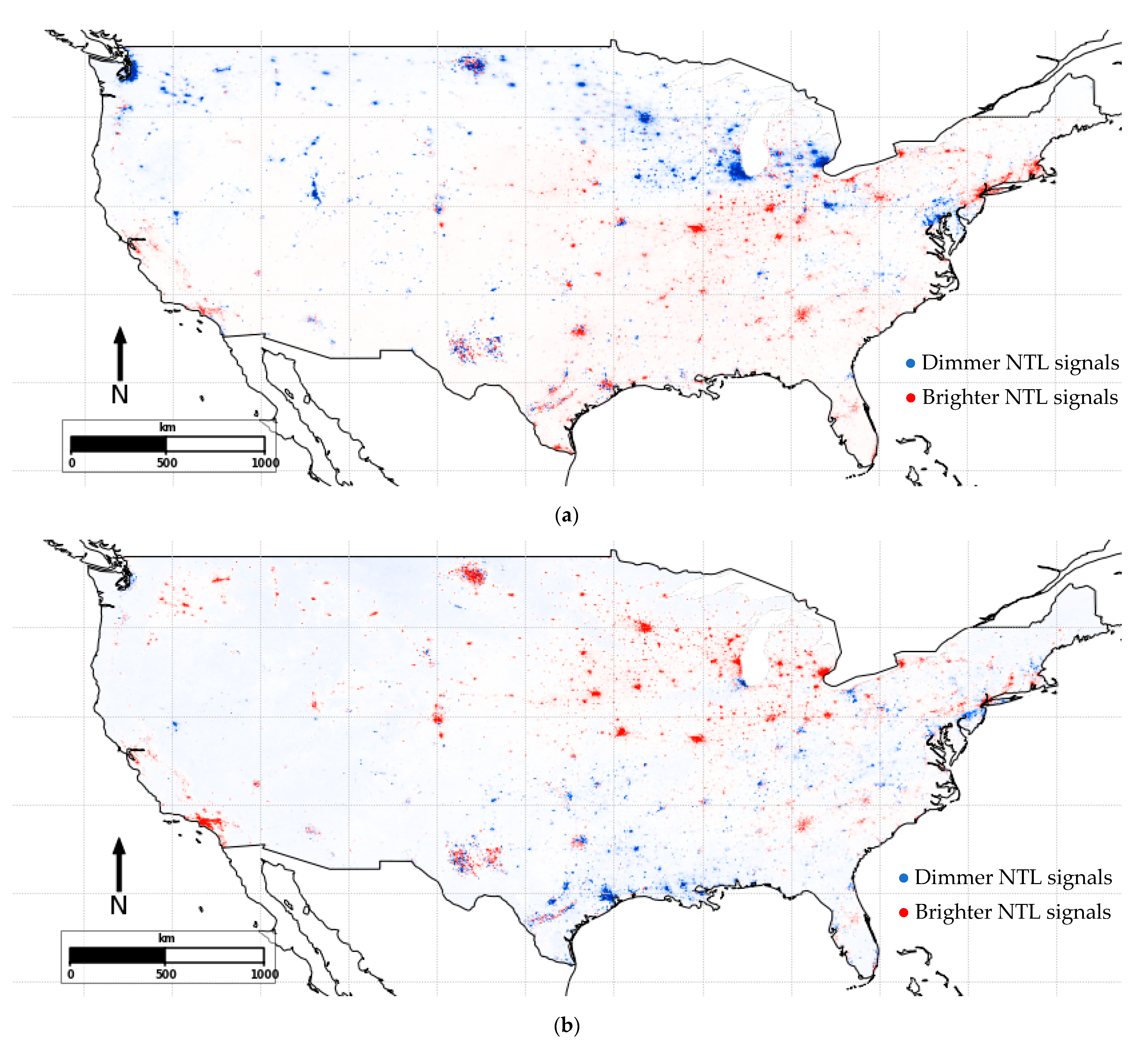
In the case of the US, a visual inspection of the NTL data recorded by VIIRS in March 2020, which was the starting point of the COVID-19 pandemic in the US, shows a sharp decline in the amount of NTL, especially in specific areas, compared to that in the pre-pandemic periods in February 2020, as well as in March 2019 (Figure 1a,b, respectively). This decline contrasts with the increase in the amount of NTL normally that was observed before the pandemic (see, for instance, Figure 2 comparing similar pre-COVID periods). Additionally, the question is whether NTL dynamics remain a reliable proxy of the GDP levels’ dynamics at the subnational level during times of upheaval. The present paper aims to answer this question.

The observed striking difference in the dynamics of the amount of NTL used after the onset of the pandemic might indicate the impact of the COVID-19 lockdowns on the economy. The question, however, remains to which extent NTL data can still serve as a proxy for the economic performance of the regions during crises. The present paper aims to answer this question. In the analysis, we compare the US state-level quarterly dynamics of the GDP during 2014–2021 with the pre-processed quarterly averaged monthly composites of the NTL data measured by VIIRS. We also assess the pandemic-induced state-level GDP losses and try to explain them using the socio-economic characteristics of the areas. The present analysis is conducted in several steps. Firstly, we compare the pre-processed years, 2014–2021, with the corresponding quarterly GDPs at the state level in the US. For this reason, we build mixed linear models linking the GDP with the NTL data separately for the pre-COVID-19 period and the whole time period. We show that not accounting for COVID-19 dummies worsens the fit of the model built for the whole time period. Secondly, we use the pre-COVID-based model to make post-pandemic GDP predictions and estimate the state-level losses by comparing those predictions with actual quarterly GDPs in the years 2020 and 2021. Finally, we try to explain the outstanding vulnerability to the crisis of states. For this reason, we run multivariate regressions linking the socioeconomic characteristics of localities with the magnitude of their economic losses. The rest of the paper is structured as follows: Section 2 describes the data and methods used in the analysis, Section 3 presents empirical results, and Section 4 discusses the obtained results and concludes the paper.

2. Materials and Methods

2.1. Data Used

2.1.1. NTL Data Source and Their Processing

In the present analysis, we used the monthly cloud-free composites of the Visible Infrared Imaging Radiometer Suite (VIIRS) Day/Night Band (DNB) NTL data collected jointly by NASA and NOAA and distributed by the Earth Observation Group (EOG) [33]. Particularly, we used a stray-light-corrected version of the NTL data, ensuring more data coverage towards the poles. The utilized NTL data have a 15 arc-second (~500 m at the Equator) spatial resolution and report average monthly and daily observations of the NTL radiance (in nW/cm²/sr) [33]. A copy of the NTL data stored on Google Earth Engine databases [32] were used in this study for the ease of performing an analysis using Python software.

VIIRS/DNB NTL data were chosen over the older Defense Meteorological Satellite Program (DMSP) NTL data due to their availability at a higher frequency, spatial resolution, higher dynamic range, and low-light detection capabilities, with the presence of on-board calibration and the absence of saturation [34].

The NTL data utilized in this analysis cover 48 contiguous states and the District of Columbia (DC) (we excluded from the analysis Alaska, Hawaii, and Puerto Rico states due to their geo-locations and expectedly inaccurate NTL data contributed by volcanic activities and auroras) spanning eight years from January 2014 to December 2021 (which represents 96 monthly composites of stray-light-corrected NTL data).

To exclude non-reliable NTL data from the analysis, the procedure of filtering out low cloud-free coverage and low average radiance, thus avoiding background noise, described in [26] was performed. Thus, from each NTL composite, we excluded pixels that in at least one dataset—within a certain quarter—had: (i) ≤2 cloud-free observations and (ii) an ≤0 NTL level. Afterward, for each NTL composite, for each state, the numbers of the filtered-out pixels were calculated, and if more than 5% of the original pixels filtered out in a state, it was excluded from the analysis.

Using the filtered NTL data, we calculated the sum of light (SoL) for each state and each monthly NTL composite. For this reason, we summed up the latitude-adjusted NTL radiances of the pixels [26] within the administrative boundary of a state. Finally, for the comparability with the GDP data, which are available quarterly (see Section 2.2), we calculated the quarterly SoLs by summing up the three monthly SoLs, which make up the corresponding quarter.

2.1.2. Socio-Economic Characteristics of the States

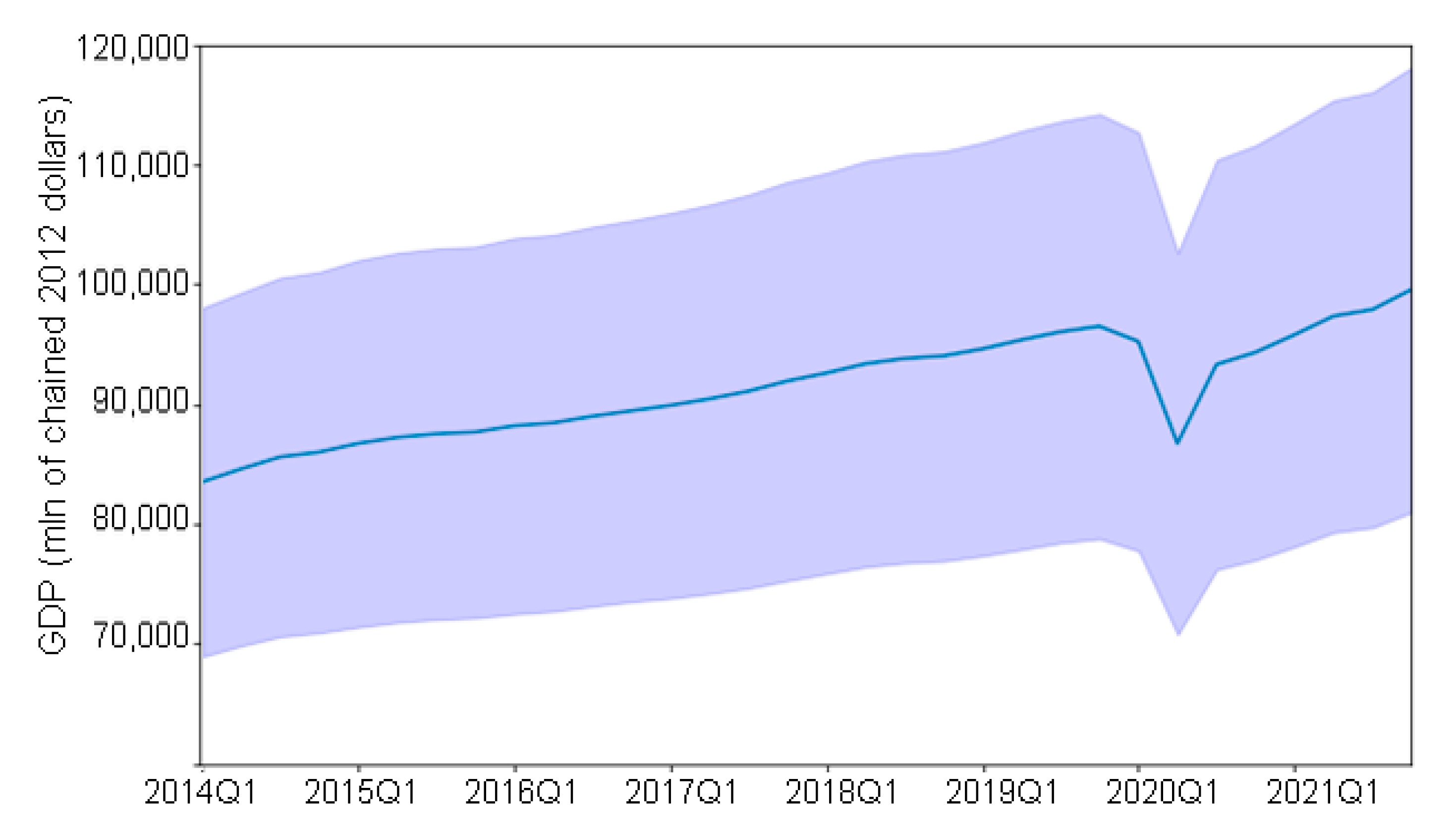
To compare the dynamics of the GDP with the processed NTL data measured by VIIRS (see Section 2.1), we used the quarterly GDP at the state level measured in millions of chained 2012 dollars, which we obtained from the Bureau of Economic Analysis [35]. As the provided data were scaled to the annual GDP, we divided the given values by four to obtain a quarterly average. Figure 3 reports the average state quarterly GDP for 2014–2021.

To assess the pandemic-induced state-level GDP losses and explain their variation across the states, we used state-level socio-economic characteristics, such as initial development level and sectoral composition, as well as the racial and ethnic composition of the states. The initial development level was assessed as GDP per capita (millions of chained 2012 dollars per person). It is established in the literature that economically stronger regions tend to better cope with crises (see, for example, [36,37]), and we expected the initial pre-pandemic GDP per capita to be negatively correlated with the pandemic loss. Sectoral specialization across regions is known to influence the magnitude of economic impact. A recent study showed that areas with a diversified structure or those specialized in sectors such as information and technology suffered less, while states concentrated in tourism suffered more [38]. In the present analysis, the sectoral compositions were calculated as fractions of the total state GDPs contributed by a certain sector of the economy. We mainly tested the service sectors that were highly impacted by the lockdowns, such as those which require in-person work, and the sectors that are resilient to lockdown, such as those which can easily switch to remote work, and states with a large fraction of highly impacted sectors that were expected to experience large loss and states with a large fraction of resilient sectors that were expected to experience small losses. Finally, the pandemic is likely to have different impacts on different ethnic groups [39,40]. In the present analysis, racial and ethnic compositions were measured as a fraction of the total state population. We defined the fraction of non-white people to be the fraction of the minority and predicted that the fraction would correlate positively with the pandemic loss. In the analysis, we also tested other socio-economic variables, such as age, gender structure, education, poverty, and unemployment levels, as well as population densities; these variables, however, were statistically insignificant in the tested models (with p > 0.1)

GDP data including industry shares were obtained from the BEA [35]. Statistics regarding population, age, and racial composition were obtained from the US Census site [41].

2.2. Methodology

In the first stage of the analysis, we linked the state-level quarterly GDPs (Section 2.2) to the corresponding state-level quarterly SoLs (Section 2.1). For this reason, we initially developed a linear mixed effects model to use NTL as a proxy for GDP in the following form:

$$\log \left(GD{P}_{i,t}\right)=\alpha +\beta \log \left(So{L}_{i,t}\right)+{{\displaystyle \sum }}_{q=2}^4{\delta }_q{Q}_q+\gamma {\mathit{Year}}_{\mathrm{adj}}+{\mu }_i+{ϵ}_{i,t}$$

(1)

where log(x) stands for the natural logarithm of x; SoL_i,t stands for the sum of lights in the i^th state for the t^th time period; Q_q stands for the quarterly dummies using Q₁ as a reference, and it is implied to account for seasonal NTL changes; Year_adj stands for the year minus 2013 (so, the series starts with a value 1 in the year 2014), and it is implied to account for long-term dynamics of the NTL; µ_i is the time-invariant state effects; ϵ_i,t is the error. We should stress, here, that the aim of the present model’s specification—common to economic studies, which use NTL data as a proxy for economic development of the regions [9]—is to check whether the NTL data are still a reliable proxy for the real GDP during a pandemic also.

For this reason, we first applied this model to the period prior to the pandemic (2014–2019 only), as well as to the whole period under analysis (2014–2021). By doing so, we aimed to show that the standard model’s fit became lower when we applied it to the whole period due to the force majeure event breaking down the ‘natural’ dynamics of the NTL intensities.

To account for the pandemic impact, we expanded upon the model (see Equation (1)), introducing to it eight additional interactive terms between the year and quarter dummies in 2020 and 2021:

$$\begin{gathered} \log \left(GD{P}_{i,t}\right)=\alpha +\beta \log \left(SO{L}_{i,t}\right)+{{\displaystyle \sum }}_{q=2}^4{\delta }_q{Q}_q+\gamma {\mathit{Year}}_{\mathrm{adj}} \\ +{{\displaystyle \sum }}_{q=1}^4{\rho }_q{Y}_{2020}{Q}_q+{{\displaystyle \sum }}_{q=1}^4{\varphi }_q{Y}_{2021}{Q}_q+{\mu }_i+{ϵ}_{i,t} \end{gathered}$$

(2)

These new variables describe pandemic season-specific deviations from the ‘normal’ seasonal dynamics separately for the two pandemic years. This analysis was conducted in Python software. For all of the models, the parameters were estimated using a maximum likelihood approach.

In the second stage of the analysis, to assess the pandemic-induced GDP losses in the states, we used the model (Equation (1)) built for the 2014–2019 period. From this model, we calculated the GDP predictions for the quarters within 2020–2021 and compared them with the corresponding actual GDP values. We calculated three metrics to measure the economic impact: maximum loss, total loss, and the number of quarters until GDP recovery to the 4th quarter (Q4) of 2019. Maximum loss is defined as the largest single difference for any quarter between the counterfactual GDP and observed GDP. This measure intends to capture the magnitude of economic loss at the trough (peak of the pandemic). Total loss is defined as the sum of the positive differences between the predicted counterfactual GDP and the observed GDP in each quarter between 2020 Q1 and 2021 Q4 until the state’s observed GDP recovers to the counterfactual GDP level. For the states whose GDP did not recover until 2021 Q4, the total loss is the sum of the positive differences of all of the eight quarters between 2020 Q1 and 2021 Q4. This measure intends to capture the magnitude of economic loss before the economy returned to the pre-pandemic growth trajectory during the period after the onset of the pandemic. The number of quarters until recovery to the 2019 Q4 levels measures the number of quarters each state took until their GDP returned to the pre-pandemic GDP level, with 2020 Q1 defined as t = 0. For example, if a state recovered to its GDP level in 2019 Q4 in 2020 Q4, the number of quarters until recovery is 3. This measure intends to capture the speed of the recovery. For this, it is worth emphasizing that the calculated losses are estimates only, and they can not be validated explicitly, although their quality, which was evaluated proceeding the performance of the models, was used for the prediction of GDP (Equations (1) and (2)).

In the final stage of the analysis, we examined the association between the socio-economic characteristics of the states and the magnitude of loss and the speed of recovery. For this reason, we performed a cross-section analysis for the 48 contiguous states and DC with three sets of regressions, with the dependent variables being the maximum loss, the total loss, and the number of months before recovering to the 2019 Q4 level. As independent variables, we used the initial development level, the racial and ethnic composition, and the sectoral composition (see Section 2.2). To control for potential endogeneity, we introduced a lagged value (the year 2019) for the independent variables. The regression is presented as follows:

$$\log \left(PI{V}_i\right)=\mathsf{\alpha }+\mathsf{\beta }\log \left(GDPp{c}_i\right)+\mathsf{\gamma }{\left(\log \left(GDPp{c}_i\right)\right)}^2+\mathsf{\delta }\log \left(m_i\right)+\mathsf{\sigma }\log \left(h{s}_i\right)+\mathsf{\omega }\log \left(l{s}_i\right)+{ϵ}_i$$

(3)

where PIV_i stands for the pandemic impact variable (either the maximum loss, the total loss, or the number of quarters until GDP recovery) in the i^th state; GDPpc stands for per capita GDP in the 2019 pre-pandemic year; m represents the minority ratio, which is calculated as the fraction of the non-white population; hs represents the fraction of GDP contributed by services with a high incidence of remote working, such as those related to information, finance and insurance, real estate and rental and leasing, professional, scientific, and technical services; ls represents the fraction of GDP contributed by services with a low incidence of remote working, such as those related to accommodation and food services, arts, entertainment, and recreation. Additionally, to address the potential effects of the spatial autocorrelation, we examined spatial error and spatial lag models. The analysis was performed in the GeoDa 1.8.x software [42].

3. Results

3.1. NTL–GDP Association

The NTL data filtering of low cloud-free coverage and low average radiance (see Section 2.1) resulted in a decrease in the number of observations from 1568 (four quarters in eight years for 48 states and DC) to 1244, which is a ~20% decrease. Most of the decreased values were for 2015 or 2016 or the summer months or a few states such as Wyoming and Oregon.

The regression results (see Equation (1) in Section 2.2) of the association between GDP and NTL data for the pre-pandemic years, 2014–2019, and for the whole of the 2014–2021 period are represented in the first two columns in

Table 1. Association between GDP and NTL before and after the COVID-19 pandemic.

Predictors and Summary Statistics	Model 1: Log(GDP), yy 2014–2019	Model 2: Log(GDP), yy 2014–2021	Model 3: Log(GDP), yy 2014–2021
Log(SoL)	0.013 ** (2.08)	0.010 (1.37)	0.025 *** (4.01)
Year adjusted	0.016 *** (31.91)	0.117 *** (25.72)	0.015 *** (27.92)
Q2 dummy	0.010 *** (3.64)	−0.004 (−1.39)	0.013 *** (4.45)
Q3 dummy	0.163 *** (5.44)	0.012 *** (3.63)	0.020 *** (6.40)
Q4 dummy	0.019 *** (7.73)	0.017 *** (5.96)	0.020 *** (7.70)
2020 * Q1 dummy	-	-	−0.001 (−0.26)
2020 * Q2 dummy	-	-	−0.107 *** (−22.60)
2020 * Q3 dummy	-	-	−0.037 *** (−7.97)
2020 * Q4 dummy	-	-	−0.030 *** (−5.93)
2021 * Q1 dummy	-	-	−0.014 ** (−2.47)
2021 * Q2 dummy	-	-	−0.012 ** (−2.34)
2021 * Q3 dummy	-	-	−0.013 *** (−2.71)
2021 * Q4 dummy	-	-	−0.005 (−0.90)
Constant	10.629 *** (77.83)	10.685 *** (72.02)	10.457 *** (74.64)
R2 within	0.60	0.42	0.62
R2 between	0.02	0.01	0.03
R2-adjusted	0.35	0.18	0.37
Number of obs.	897	1244	1244

Note: * stands for p < 0.1; **—for p < 0.05; ***—for p < 0.01. t-statistics in parentheses. The random effects estimations are applied following the results of the Breusch and Pagan LM test and Hausman test.

(Models 1 and 2, correspondingly). The results show that the SoL is positively associated with the GDP in a significant manner (t = 2.08; p < 0.05) in the pre-pandemic period, 2014–2019 (see Model 1 in Table 1). A positive coefficient for the year indicates a positive association with an increasing trend of the GDP over the years. Similarly, positive coefficients of the quarterly dummies for Q2–Q4 (with Q1 as the reference point) capture the seasonality and show that the GDP value is higher for a given value of SoLs in Q2 compared with that in Q1, and the difference in Q3 and Q4 is even bigger compared to that in Q1, which are all consistent with the literature on the variation of the NTL data [30,43,44].

Our analysis also shows that a mechanistic extension of the model (Equation (1)) to 2020–2021 after the onset of the pandemic results in a poorer fit of the model (with R²-adjusted 0.18 vs. 0.35—see Models 1 and 2 in Table 1). Due to this, the association between GDP and NTL is insignificant (t = 1.37; p > 0.1). In the meantime, accounting for the COVID-19 phenomenon (see Equation (2) in Section 2.2) shows that the association between GDP and NTL is positive and significant (t = 4.01; p < 0.01—see Model 3 in Table 1), and the model fit essentially improves (R² adjusted from 0.18 to 0.37). Notably, the effects of the main predictors in the extended model (see Model 3 in Table 1)—SoL, year, and seasons—appear to be close to those in the initial pre-COVID model (Model 1 in Table 1). Due to this, the association between GDP and NTL is stronger, as manifested by the higher significance of the corresponding effect (t = 4.01 in Model 3 vs. t = 2.08 in Model 1). As expected, the coefficients of the interactive terms that capture the quarter-specific impacts of COVID-19 are all negative. The magnitude of the interactive term 2020*Q2 (which is the beginning of the lockdown in the US) indicates the extremely large negative shock (t = −22.60; p < 0.01) to the economy that occurred at the time when the COVID pandemic began. The magnitude of the coefficients of 2020*Q3 and 2020*Q4 also remained imposing (t < −5.93; p < 0.01), but these are only ~30–40% of the magnitude of the 2020*Q2 coefficient. This signals the prolonged large negative impact and nascent rebound. The magnitude of the coefficients in Q1–Q4 in 2021 are essentially smaller, but they remain negative. Due to this, the last coefficient 2021*Q4 is as insignificant (t = −0.90; p > 0.1), meaning that the last quarter of 2021 already behaves as a typical non-COVID fourth quarter does.

3.2. State-Wise Economic Losses Due to the Pandemic

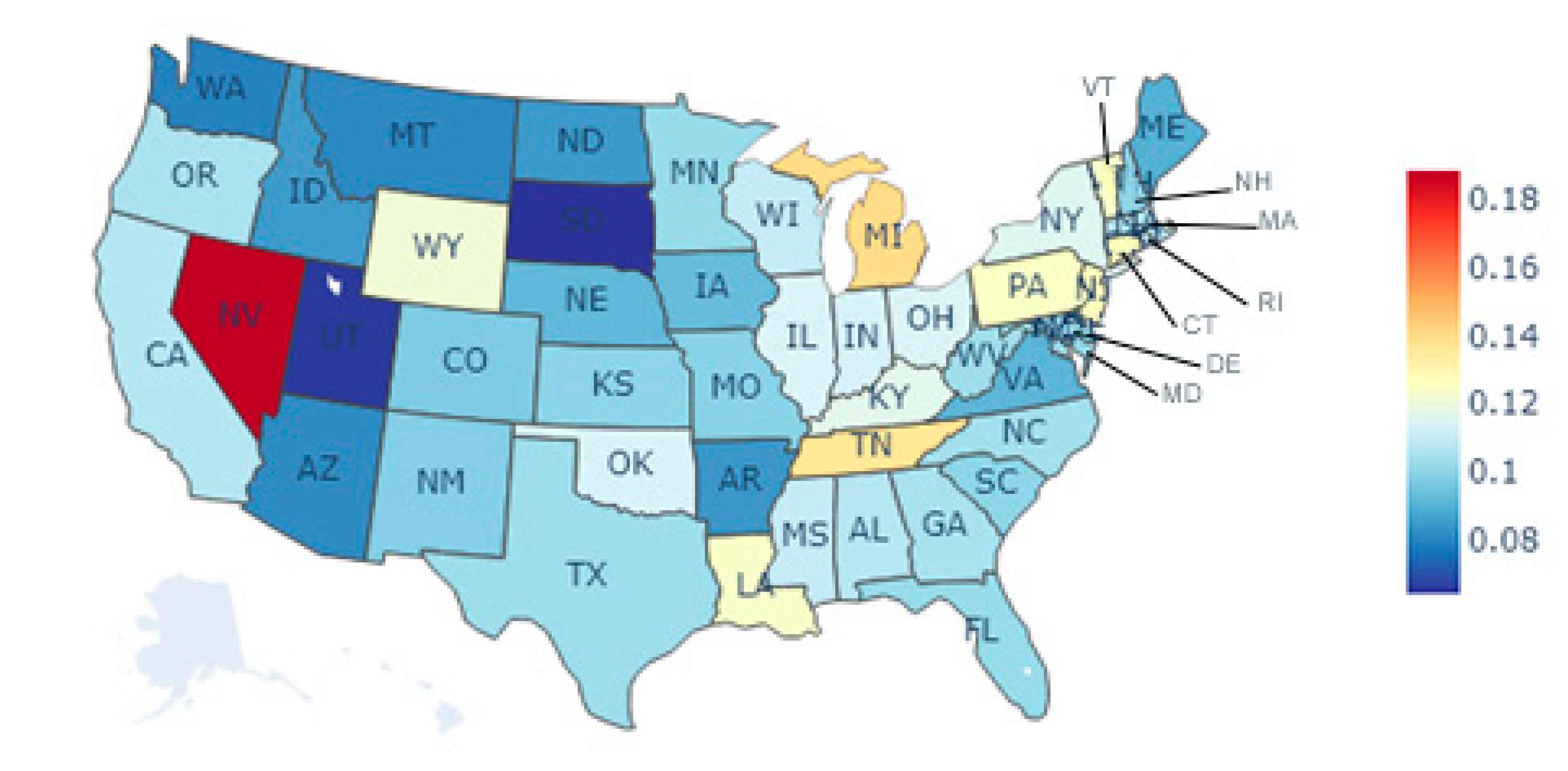
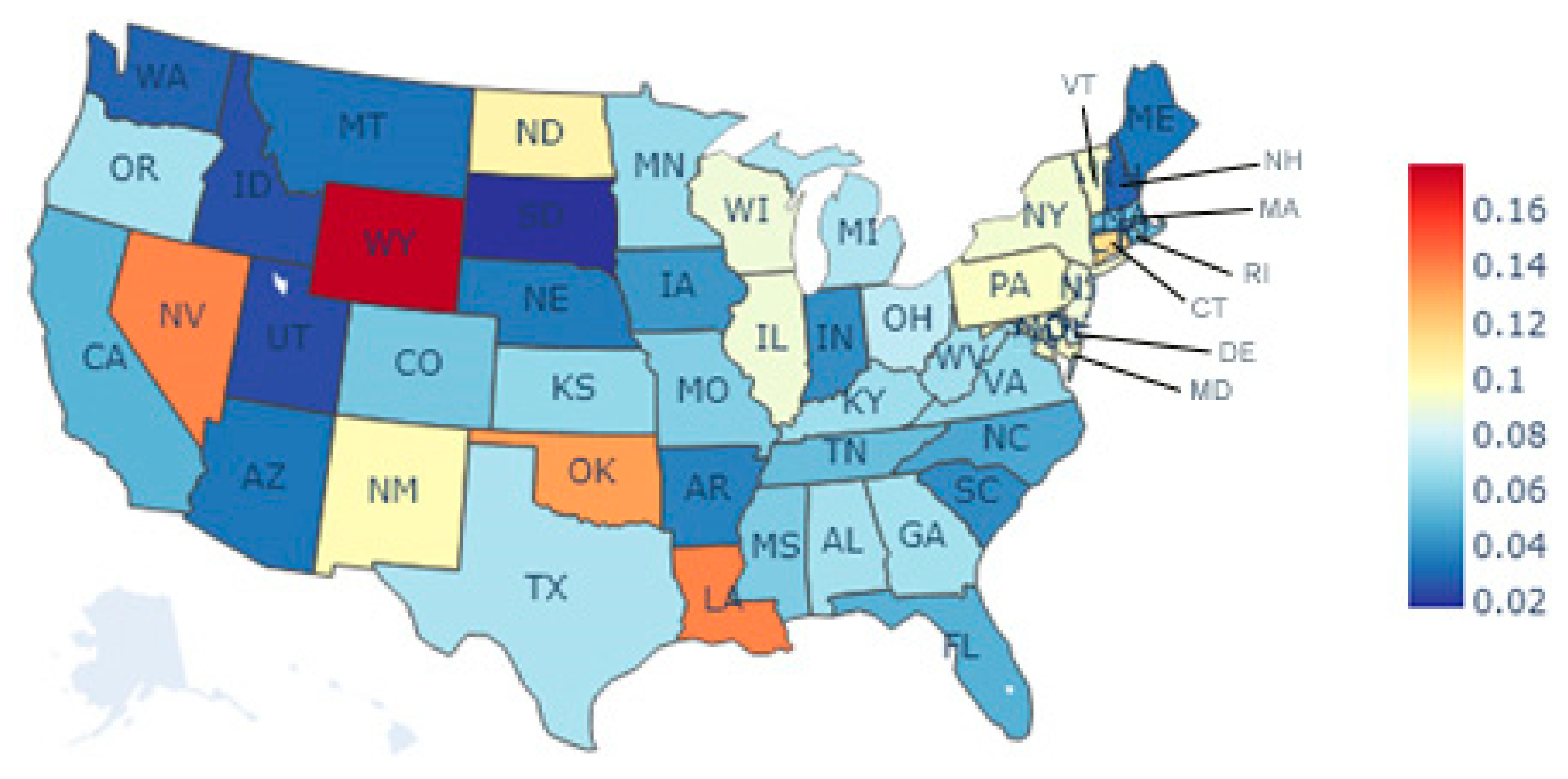
The state-wise pandemic impact in the present analysis was measured by the magnitude of the estimated economic losses, either in terms of the maximum loss, the total loss, or the number of quarters until the GDP recovered to the level of the 4th quarter of 2019 (see Section 2.2). Thus, Figure 4 reports the maximum loss of the quarterly GDP of each state after the pandemic as a ratio to its 2019 Q4 GDP level. For most of the states, the ratio has a range of ~10–15%. Figure 5 shows the total loss of GDP of each state until its recovery to the pre-pandemic level as a share of its 2019 GDP. For most of the states, the ratio ranges from ~5% to ~15%. The results show that Nevada suffered the largest maximum loss (~18%—see Figure 4) and total loss (~15%—see Figure 5), which could be related to the heavy hit to tourism industries in Las Vegas due to COVID-19.

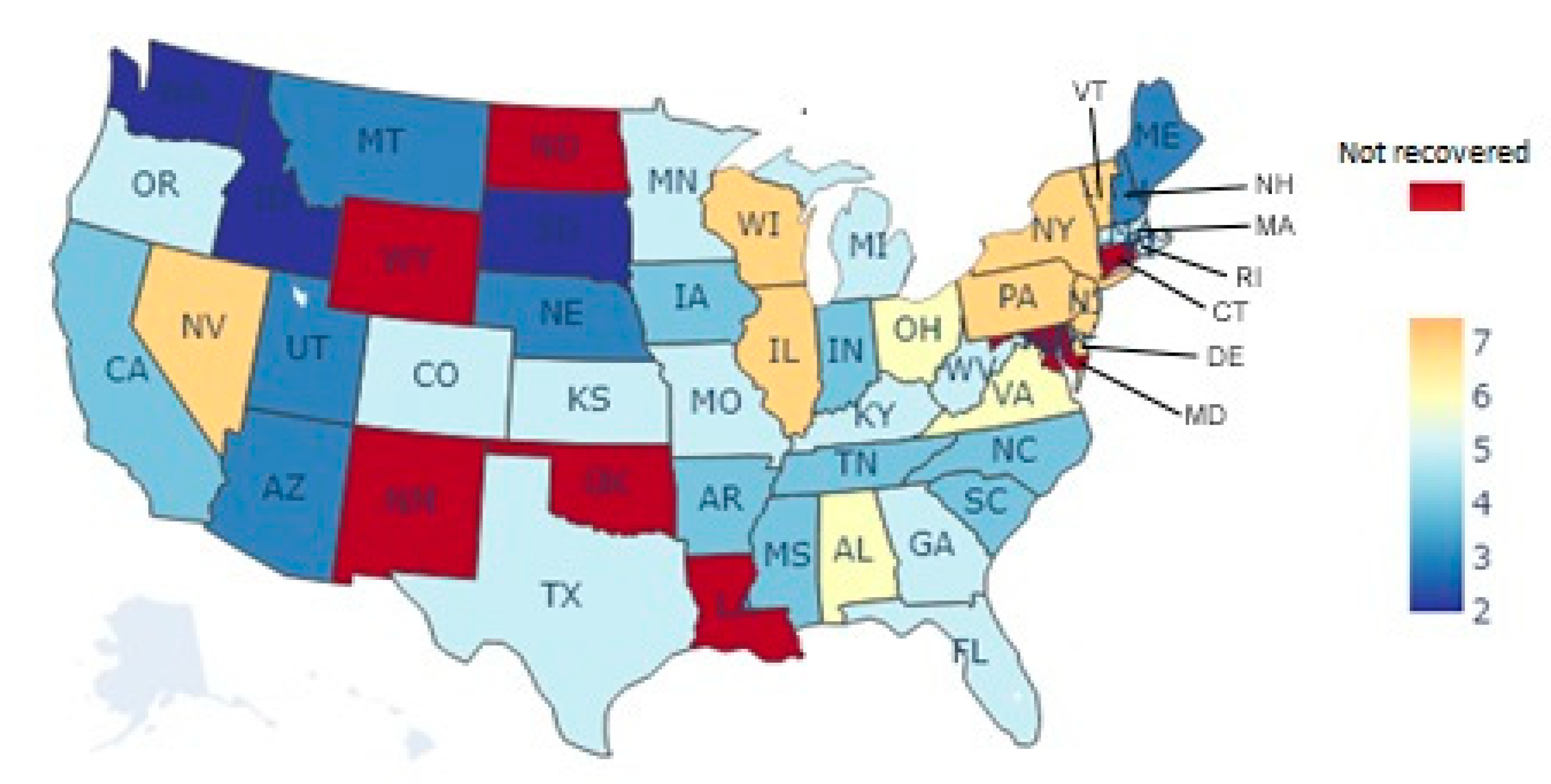
Figure 6 reports the number of quarters it took for each state to recover to the pre-pandemic GDP in the 4th quarter of 2019. While it took from two to seven quarters for most of the states to recover to the pre-pandemic level GDP, seven states, including Connecticut, Louisiana, Maryland, New Mexico, North Dakota, Oklahoma, and Wyoming, did not recover before the end of the analyzed period (the 4th quarter of 2021). This demonstrates the severity of the COVID shock on the economy and the challenges to post-pandemic recovery. The results reported in Figure 6 largely corroborate the findings in Figure 4 and Figure 5, pointing out that states experiencing larger maximum losses and less speedy recoveries often suffer larger total losses.

3.3. Socio-Economic Characteristics vs. State-Wise Economic Losses

Table 2. Association between the magnitude of the economic losses and socioeconomic characteristics of the states (model type: linear regression).

Predictors and Summary Statistics	Model 4: Log(Max Loss)	Model 5: Log(Total Loss)	Model 6: Log(N. of Quarters)
2019 GDPpc (log)	−4.284 *** (−4.47)	−7.345 *** (−2.95)	−4.683 ** (−2.28)
2019 GDPpc (log, squared term)	−0.789 *** (−4.37)	−1.522 *** (−3.24)	−0.979 ** (−2.52)
Minority ratio (log)	0.134 *** (2.94)	0.401 *** (3.40)	0.305 *** (3.13)
Services with the remote working opportunities (log)	−0.292 ** (−2.45)	−1.233 *** (−3.99)	−0.723 *** (−2.83)
Services with the limited remote working opportunities (log)	0.424 *** (4.03)	0.492 * (1.80)	0.262 (1.16)
Constant	−6.924 *** (−5.90)	−10.586 *** (−3.47)	−3.295 (−1.31)
R2	0.404	0.385	0.306
R2-adjusted	0.335	0.314	0.226
Moran’s I	3.306 ***	1.065	2.376 **
Number of obs.	49	49	49

Note: * stands for p < 0.1; **—for p < 0.05; ***—for p < 0.01. t-statistics in parentheses.

displays the results of the association between the socio-economic characteristics of the states and pandemic-induced economic losses, which are represented by either the maximum loss, the total loss, or the number of quarters until the GDP recovered to the level of the 4th quarter of 2019 (see Section 2.2). For all of the reported models, the variance of the inflation factor for all of predictors did not exceed 1.5, with acceptable multicollinearity between the explanatory variables.

Table A1. Database for the analysis of the association between the socio-economic characteristics of the states and pandemic-induced economic losses (represented by either maximum loss, total loss, or the number of quarters until GDP recovered to the level of the 4th quarter of 2019). See Section 2.2 and Section 3.3 for the explanation.

State	Maximum Loss	Total Loss	Quarters Until Recovery	GDP pc	Minority %	Share of High Services	Share of Low Services
AL	0.107	0.069	6	0.041	0.309	0.249	0.052
AZ	0.081	0.035	3	0.044	0.174	0.319	0.060
AR	0.084	0.038	4	0.039	0.210	0.208	0.054
CA	0.107	0.052	4	0.069	0.281	0.386	0.057
CO	0.097	0.059	5	0.062	0.131	0.359	0.065
CT	0.127	0.114	8	0.071	0.203	0.415	0.050
DE	0.096	0.084	7	0.066	0.308	0.496	0.040
DC	0.072	0.071	6	0.176	0.540	0.400	0.112
FL	0.102	0.051	5	0.045	0.227	0.359	0.080
GA	0.105	0.069	5	0.053	0.398	0.378	0.046
ID	0.085	0.026	2	0.041	0.070	0.252	0.054
IL	0.114	0.091	7	0.061	0.232	0.349	0.060
IN	0.113	0.041	4	0.050	0.152	0.221	0.054
IA	0.093	0.044	4	0.055	0.094	0.290	0.046
KS	0.100	0.065	5	0.055	0.137	0.278	0.046
KY	0.117	0.068	5	0.043	0.125	0.228	0.054
LA	0.124	0.140	8	0.051	0.372	0.215	0.055
ME	0.090	0.035	3	0.044	0.056	0.295	0.071
MD	0.103	0.095	8	0.061	0.415	0.354	0.057
MA	0.107	0.056	5	0.075	0.194	0.420	0.057
MI	0.140	0.072	5	0.047	0.208	0.291	0.054
MN	0.102	0.067	5	0.060	0.162	0.303	0.050
MS	0.110	0.061	4	0.034	0.409	0.205	0.063
MO	0.099	0.062	5	0.047	0.171	0.303	0.061
MT	0.081	0.034	3	0.044	0.111	0.255	0.068
NE	0.092	0.036	3	0.061	0.119	0.287	0.043
NV	0.189	0.139	7	0.051	0.261	0.278	0.167
NH	0.100	0.030	3	0.057	0.069	0.348	0.073
NJ	0.127	0.090	7	0.063	0.281	0.359	0.049
NM	0.098	0.100	8	0.045	0.181	0.240	0.061
NY	0.116	0.092	7	0.077	0.304	0.494	0.063
NC	0.104	0.048	4	0.049	0.294	0.304	0.055
ND	0.084	0.103	8	0.074	0.131	0.191	0.039
OH	0.114	0.075	6	0.052	0.183	0.287	0.052
OK	0.114	0.133	8	0.051	0.260	0.189	0.048
OR	0.105	0.070	5	0.052	0.133	0.290	0.061
PA	0.125	0.095	7	0.056	0.184	0.325	0.053
RI	0.109	0.058	5	0.050	0.164	0.316	0.069
SC	0.100	0.040	4	0.041	0.314	0.271	0.065
SD	0.064	0.018	2	0.053	0.154	0.296	0.053
TN	0.136	0.055	4	0.048	0.216	0.267	0.079
TX	0.103	0.071	5	0.062	0.213	0.263	0.046
UT	0.065	0.024	3	0.053	0.094	0.328	0.057
VT	0.123	0.094	7	0.048	0.058	0.287	0.083
VA	0.091	0.065	6	0.057	0.306	0.366	0.055
WA	0.079	0.030	2	0.070	0.215	0.396	0.050
WV	0.103	0.068	5	0.040	0.065	0.194	0.052
WI	0.110	0.090	7	0.052	0.130	0.283	0.052
WY	0.121	0.177	8	0.067	0.075	0.168	0.049

and

Table A2. Pearson’s correlations between socio-economic characteristics of the US states used in the analysis (see Table 2).

	Year 2019 GDPpc (log)	Minority Ratio (log)	Services with the Remote Working Opportunities (log)	Services with the Limited Remote Working Opportunities (log)
2019 GDPpc (log)	1.00
Minority ratio (log)	0.27	1.00
Services with the remote working opportunities (log)	0.50	0.31	1.00
Services with the limited remote working opportunities (log)	0.06	0.08	0.12	1.00

in Appendix A report the database and correlations between the analyzed predictors.

While we were running the models, for the seven states whose GDP did not recover to the 2019 Q4 level until 2021 Q4 (see Figure 5 in Section 3.2), the number of quarters until the recovery to the 2019 Q4 GDP was artificially assumed to be eight. This assumption was made to keep all of 49 states in the regression without excluding the states that experienced the least speedy recoveries.

As it can be seen from the table, the states with a higher GDP per capita before the COVID-19 pandemic typically experienced smaller maximum and total losses, as well as shorter recovery periods (to see a statistically significant negative association between the three metrics and 2019 GDP per capita (t < −2.28; p < 0.05), see Models 4–6 in Table 2). Our results also indicate that states with a higher ratio of services that were paid better and employed remote working opportunities experienced smaller losses (t < −2.45; p < 0.05), while the states with a higher ratio of services with limited remote work opportunities generally suffered more losses (t > 1.8; p < 0.1). Additionally, the states with higher minority rates suffered larger economic losses and a less speedy recovery (t > 2.94; p < 0.01).

For two out of three models, the effect of spatial autocorrelation was not negligible (with Moran’s I > 2.376; p < 0.05).

Table 3. Association between the magnitude of the economic losses and socioeconomic characteristics of the states (model type: spatial error regression).

Predictors and Summary Statistics	Model 4a: Log(Max Loss)	Model 5a: Log(Total Loss)	Model 6a: Log(N. of Quarters)
2019 GDPpc (log)	−4.014 *** (−5.86)	−7.330 *** (−3.32)	−5.085 *** (−3.17)
2019 GDPpc (log, squared term)	−0.762 *** (−5.85)	−1.525 *** (−3.65)	−1.057 *** (−3.47)
Minority ratio (log)	0.107 ** (2.16)	0.376 *** (3.10)	0.244 ** (2.26)
Services with the remote working opportunities (log)	−0.514 *** (−5.20)	−1.431 *** (−4.89)	−1.081 *** (−4.75)
Services with the limited remote working opportunities (log)	0.436 *** (5.48)	0.525 * (2.10)	0.333 * (1.79)
Constant	−6.651 *** (−7.79)	−10.699 *** (−3.92)	−4.132 ** (−2.07)
λ	0.615 *** (4.98)	0.224 (1.22)	0.516 *** (3.62)
R2	0.574	0.401	0.427
Number of obs.	49	49	49

Note: * stands for p < 0.1; **—for p < 0.05; ***—for p < 0.01. z-statistics in parentheses.

reports spatial error models (they are better fit and have more generality compared to their spatial lag counterparts). As it can be seen from the table, the spatial error model results are remarkably close to the values of the coefficients for the main predictors (compare models in Table 3 and Table 2), although the overall fit appears to be better (R² = 0.401–0.574 vs. R² = 0.306–0.404).

4. Discussion

In this paper, we have used the latest set of monthly night-time light (NTL) composites from VIIRS/DNB from 2014 to 2021 to examine the relationship between NTL and the economic activities in the U.S. and measure the pandemic’s impact on the economy at the state level. In the core analysis, we first examined the relationships within the latitude-adjusted NTL data, which were filtered on the low cloud-free coverage and low average radiances, for the state-level GDP over the pre-pandemic period (from 2014 to 2019) on a quarterly basis. Secondly, we extended the model to the pandemic period (from 2020 to 2021) with additional control variables to account for the shock caused by COVID and assessed the economic loss compared with the counterfactual GDP estimate (in the absence of COVID-19). Finally, we elaborated on the association between the socio-economic characteristics of the states and the magnitude of their economic loss and the speed of recovery. Several recent studies explored NTL dynamics during the COVID-19 pandemic and concluded that drastic changes did take place [26,27,28]; some studies have confirmed that the NTL data correlate with GDP in the pandemic period at the level of selected cities [29] and at the national level [30,31]. Our study adds value by using the NTL to measure the changes in the quarterly GDP at the subnational level in the U.S. before and during the pandemic period. An important finding of our analysis is that NTL data, as they do in the ‘normal period’, remain a reliable proxy for the economic development of the regions at the subnational level even under external shocks. Our analysis also sheds light on the characteristics of the regions that are the most vulnerable—in terms of economic losses and the speed of recovery—to COVID-19.

The results of the association of the quarterly NTL data and GDP at the state level, which were controlled for the seasonal and long-term NTL changes, indicate a significantly positive GDP–NTL association in pre-pandemic period (t = 2.08; p < 0.05, see Model 1 in Table 1), with the model fit achieving R² = 0.60. These numbers corroborate the previous findings in the literature that NTL is a reliable proxy for GDP at the subnational level in the ‘normal period’. Thus, in their recent comprehensive analysis, Gibson and Boe-Gibson report a fit of R² = 0.35–0.70 for GDP-NTL association models based on the US 2014–2019 state-level data and different versions of annual NTL composites [9].

Our results indicate that NTL may remain a reliable GDP proxy—at least to the same extent as it does in ‘normal periods’—even after large external shocks (such as the pandemic in 2020 and 2021), given that the effect of COVID is referred to via using the interactive terms of year and quarter dummies. The GDP–NTL association in our analysis was significantly positive (t = 4.01; p < 0.01, see Model 3 in Table 1), and the model fit achieved R² = 0.62. These results are in line with those of the previous analysis by Roberts, reporting that at the national level, in the case of Morocco, a strong correlation between the quarterly trends in overall NTL intensity and the GDP levels existed during the pandemic [30].

While we were assessing the pandemic-induced losses and the time of recovery, we applied an accepted form of analysis using satellite NTL data to study the dimming and recovery of lights after exogenous shocks, such as natural disasters and conflicts (see, for example, [45,46]). Thus, as our analysis indicates, the magnitude of loss due to COVID-19, as well as the speed of recovery, varied widely across the states, with most of the states’ ratio of maximum quarterly loss ranging from ~10% to ~15% in the pre-pandemic 4th quarter in 2019, and the total GDP loss ranging from ~5% to ~15% in 2019. In the 4th quarter of 2021, 42 out of the 49 states recovered to the GDP level of the 4th quarter in 2019. These findings generally coincide with the patterns of GDP and jobs. Thus, Ettlinger, while citing the results from the September 2021 Bureau of Labor Statistics monthly survey, stated that while the U.S. as a nation, overall, has recovered close to 80% of those jobs, the rate of the recovery of the lost jobs in individual states ranges from 36% of the pre-pandemic levels to a full recovery [47].

Our results argue that the states with a lower initial pre-pandemic GDP per capita level, a higher number of low-paid services jobs with limited remote working opportunities, and a higher minority ratio suffered larger economic loss and less speedy recovery post-pandemic. This association between the socio-economic characteristics and economic losses are largely consistent with several recent studies on the pandemic’s impact on the economy in the U.S. Thus, Breaux et al. argued that while the pandemic had a drastic impact on the entire economy and people’s life, the impact varied by industry [48]. Klein and Smith [49] found that the cities with a high concentration of tourism, such as Las Vegas and Orlando, suffered the largest losses, while the cities with a high concentration of technology and information industries, such as San Francisco and Seattle, suffered less. The authors also argue that the areas with relatively large Hispanic or Latino communities were more vulnerable to the pandemic-induced consequences, probably reflecting the demographic composition of workers in heavily impacted industries [49].

In the meantime, the results of the analysis should be interpreted with caution: Firstly, the relationship between GDP and NTL is not perfect. While, typically, the NTL intensity increases as incomes rise, the imperfection of the association is due to its complexity and is conditioned by many factors [50,51], including indoor versus outdoor lighting, contributions of investment versus income, and the energy/light intensity of different productive activities. For example, the production of manufacturing products might result in a in the use of more light than the design of computer software would for the same value of GDP. Energy preservation habits and population density often play an important role as well. Gibson and Boe-Gibson show that NTL is a poor predictor of agricultural activity and changes in the total economic activity in highly agricultural counties [9]. In Mellander et al.’s study, the authors demonstrate that the link between NTL and economic activity estimated by wages is slightly overestimated in large urban areas and underestimated in rural areas [7]. The NTL data were found to be a better predictor for GDP in metropolitan statistical areas than they were for entire states, as night-time light may be more closely related to urban sectors than rural sectors [52]. In addition, the reasons a weaker association between NTL and GDP in the growth data might be related to the errors or inconsistencies in the digital image luminosities captured by satellites over time; the decay of the optical attributes of sensors affects the reliability of the radiance measures at night, and seasonal changes captured by the VIIRS, such as stray light in high-latitude regions, increases in the summer [52]. Secondly, filtering the NTL data on the low cloud-free coverage and low average radiance might affect the areas differently, which could have varied impacts on the estimates. Finally, the estimated counterfactual GDP in 2020 and 2021 is drawn from the trendline, with a slope that stands for the national average and the intercept adjusted for state-specific levels, which might underestimate or overestimate the would-be counterfactual GDP for the states with growth rates that deviate from the national average.

Future research may be focused on refining the revealed patterns in the NTL–GDP association during the pandemic at the state level. This would help us to address variations in lockdown policies across the states. It also seems promising to explore the effects of other socio-economic variables to improve the estimates of GDP losses both to improve the estimates for GDP losses in the US and to adjust the developed models beyond the study area to other countries and regions.

A potential concern may be associated with the absence of the atmospheric calibration of the used EOG-provided NTL data product. Indeed, several recent studies have reported changes in the concentrations of some pollutants during the pandemic times. Rather expectedly, the lockdown policies resulted in decreased emissions of the main atmospheric pollutants, such as carbon dioxide, nitrogen oxides, aerosols, and particulate matter [53,54] (although the opposite local effects were sometimes observed due to weather peculiarities [53]). Most of the mentioned pollutants, however, absorb electromagnetic radiation that is beyond the visible light range, and thus do not affect NTL brightness. For those pollutants that do absorb light in its visible spectrum, such as aerosols, the negative association between their concentration and atmospheric transmissivity is long understood [55]. Thus, a pandemic-induced decrease in the amount of aerosols should result in slightly brighter NTL radiances. This means that if it was observed, the lockdown-associated dimming would have had to surpass the above-mentioned brightening effect. This justifies using the EOG NTL product in studies focusing on dimming [26,27]. However, atmospheric gases are known to affect light scattering, especially in the short-wavelength range. Thus, decreased emissions of pollutants during the outbreak might lead to some dimming of the NTL. Although the impact of this effect seems minor compared to that of the economically induced changes, it should still be checked by using the atmospherically calibrated NTL, such as the Black Marble product [56].

5. Conclusions

A prompt understanding of the magnitude of the economic losses and capturing the signs of recovery is required to take swift and informed action in stressful periods. This especially holds for countries and regions where traditional measures are unavailable, infrequent, or inaccurate. The herein presented results suggest that the NTL data, which are available at high frequency at granular spatial levels for almost all of the areas on Earth and are accessible free of charge with only a short time lag, remain a reliable proxy for the economic performance of regions, even during periods of upheaval. Furthermore, comparing the statistical associations between GDP and NTL in ‘normal’ and pandemic periods allows us to assess the degree of the vulnerability/resilience of different areas to socio-economic perturbations, which would contribute to building informed precise anti-crisis policies.

References

1. Croft, T.A. Nighttime Images of the Earth from Space. Sci. Am. 1978, 239, 86–98. [Google Scholar] [CrossRef]
2. Elvidge, C.D.; Baugh, K.E.; Kihn, E.A.; Kroehl, H.W.; Davis, E.R.; Davis, C.W. Relation between satellite observed visible-near infrared emissions, population, economic activity and electric power consumption. Int. J. Remote Sens. 1997, 18, 1373–1379. [Google Scholar] [CrossRef]
3. Doll, C.H.; Muller, J.-P.; Elvidge, C.D. Night-time Imagery as a Tool for Global Mapping of Socioeconomic Parameters and Greenhouse Gas Emissions. AMBIO A J. Hum. Environ. 2000, 29, 157–162. [Google Scholar] [CrossRef]
4. Ebener, S.; Murray, C.; Tandon, A.; Elvidge, C.C. From wealth to health: Modelling the distribution of income per capita at the sub-national level using night-time light imagery. Int. J. Health Geogr. 2005, 4, 5. [Google Scholar] [CrossRef] [PubMed]
5. Elvidge, C.D.; Sutton, P.C.; Ghosh, T.; Tuttle, B.T.; Baugh, K.E.; Bhaduri, B.; Bright, E. A global poverty map derived from satellite data. Comput. Geosci. 2009, 35, 1652–1660. [Google Scholar] [CrossRef]
6. Li, X.; Xu, H.; Chen, X.; Li, C. Potential of NPP-VIIRS nighttime light imagery for modeling the regional economy of China. Remote Sens. 2013, 5, 3057–3081. [Google Scholar] [CrossRef]
7. Mellander, C.; Lobo, J.; Stolarick, K.; Matheson, Z. Night-time light data: A good proxy measure for economic activity? PLoS ONE 2015, 10, e0139779. [Google Scholar] [CrossRef]
8. Wu, R.; Yang, D.; Dong, J.; Zhang, L.; Xia, F. Regional Inequality in China Based on NPP-VIIRS Night-Time Light Imagery. Remote Sens. 2018, 10, 240. [Google Scholar] [CrossRef]
9. Gibson, J.; Boe-Gibson, G. Nighttime Lights and County-Level Economic Activity in the United States: 2001 to 2019. Remote Sens. 2021, 13, 2741. [Google Scholar] [CrossRef]
10. Sutton, P.; Roberts, D.; Elvidge, C.; Baugh, K. Census from Heaven: An estimate of the global human population using night-time satellite imagery. Int. J. Remote Sens. 2001, 22, 3061–3076. [Google Scholar] [CrossRef]
11. Amaral, S.; Monteiro, A.M.V.; Camara, G.; Quintanilha, J.A. DMSP/OLS night-time light imagery for urban population estimates in the Brazilian Amazon. Int. J. Remote Sens. 2006, 27, 855–870. [Google Scholar] [CrossRef]
12. Zhuo, L.; Ichinose, T.; Zheng, J.; Chen, J.; Shi, P.J.; Li, X. Modelling the population density of China at the pixel level based on DMSP/OLS non-radiance-calibrated night-time light images. Int. J. Remote Sens. 2009, 30, 1003–1018. [Google Scholar] [CrossRef]
13. Anderson, S.J.; Tuttle, B.T.; Powell, R.L.; Sutton, P.C. Characterizing relationships between population density and nighttime imagery for Denver, Colorado: Issues of scale and representation. Int. J. Remote Sens. 2010, 31, 5733–5746. [Google Scholar] [CrossRef]
14. Hopkins, G.R.; Gaston, K.J.; Visser, M.E.; Elgar, M.A.; Jones, T.M. Artificial light at night as a driver of evolution across urban-rural landscapes. Front. Ecol. Environ. 2018, 16, 472–479. [Google Scholar] [CrossRef]
15. Stokes, E.C.; Seto, K.C. Characterizing urban infrastructural transitions for the Sustainable Development Goals using multi-temporal land, population, and nighttime light data. Remote Sens. Environ. 2019, 234, 111430. [Google Scholar] [CrossRef]
16. Kloog, I.; Haim, A.; Stevens, R.G.; Portnov, B.A. Global co-distribution of light at night (LAN) and cancers of prostate, colon, and lung in men. Chronobiol. Int. 2009, 26, 108–125. [Google Scholar] [CrossRef]
17. Kloog, I.; Stevens, R.G.; Haim, A.; Portnov, B.A. Nighttime light level co-distributes with breast cancer incidence worldwide. Cancer Causes Control 2010, 21, 2059–2068. [Google Scholar] [CrossRef]
18. Haim, A.; Portnov, B.A. Light Pollution as a New Risk Factor for Human Breast and Prostate Cancers; Springer: Dordrecht, The Netherlands, 2013; ISBN 9789400762206. [Google Scholar]
19. Rybnikova, N.; Haim, A.; Portnov, B.A. Artificial Light at Night (ALAN) and breast cancer incidence worldwide: A revisit of earlier findings with analysis of current trends. Chronobiol. Int. 2015, 32, 757–773. [Google Scholar] [CrossRef]
20. Rybnikova, N.A.; Portnov, B.A. Outdoor light and breast cancer incidence: A comparative analysis of DMSP and VIIRS-DNB satellite data. Int. J. Remote Sens. 2017, 38, 5952–5961. [Google Scholar] [CrossRef]
21. Meng, L.; Graus, W.; Worrell, E.; Huang, B. Estimating CO2 (carbon dioxide) emissions at urban scales by DMSP/OLS (Defense Meteorological Satellite Program’s Operational Linescan System) nighttime light imagery: Methodological challenges and a case study for China. Energy 2014, 71, 468–478. [Google Scholar] [CrossRef]
22. Ou, J.; Liu, X.; Li, X.; Li, M.; Li, W. Evaluation of NPP-VIIRS nighttime light data for mapping global fossil fuel combustion CO2 emissions: A comparison with DMSP-OLS nighttime light data. PLoS ONE 2015, 10, e0138310. [Google Scholar] [CrossRef]
23. Zhao, J.; Ji, G.; Yue, Y.; Lai, Z.; Chen, Y.; Yang, D.; Yang, X.; Wang, Z. Spatio-temporal dynamics of urban residential CO2 emissions and their driving forces in China using the integrated two nighttime light datasets. Appl. Energy 2019, 235, 612–624. [Google Scholar] [CrossRef]
24. Lv, Q.; Liu, H.; Wang, J.; Liu, H.; Shang, Y. Multiscale analysis on spatiotemporal dynamics of energy consumption CO2 emissions in China: Utilizing the integrated of DMSP-OLS and NPP-VIIRS nighttime light datasets. Sci. Total Environ. 2020, 703, 134394. [Google Scholar] [CrossRef]
25. Levin, N.; Kyba, C.C.M.; Zhang, Q.; Sánchez de Miguel, A.; Román, M.O.; Li, X.; Portnov, B.A.; Molthan, A.L.; Jechow, A.; Miller, S.D.; et al. Remote sensing of night lights: A review and an outlook for the future. Remote Sens. Environ. 2020, 237, 111443. [Google Scholar] [CrossRef]
26. Elvidge, C.D.; Ghosh, T.; Hsu, F.-C.; Zhizhin, M.; Bazilian, M. The dimming of lights in China during the COVID-19 pandemic. Remote Sens. 2020, 12, 2851. [Google Scholar] [CrossRef]
27. Ghosh, T.; Elvidge, C.D.; Hsu, F.-C.; Zhizhin, M.; Bazilian, M. The dimming of lights in India during the COVID-19 pandemic. Remote Sens. 2020, 12, 3289. [Google Scholar] [CrossRef]
28. Xu, G.; Xiu, T.; Li, X.; Liang, X.; Jiao, L. Lockdown induced night-time light dynamics during the COVID-19 epidemic in global megacities. Elsevier 2021, 102, 102421. [Google Scholar] [CrossRef] [PubMed]
29. Wang, X.; Yan, G.; Mu, X.; Xie, D.; Xu, J.; Zhang, Z.; Zhang, D. Human Activity Changes During COVID-19 Lockdown in China—A View From Nighttime Light. Geohealth 2022, 6, e2021GH000555. [Google Scholar] [CrossRef] [PubMed]
30. Roberts, M. Tracking economic activity in response to the COVID-19 crisis using nighttime lights–The case of Morocco. Dev. Eng. 2021, 6, 100067. [Google Scholar] [CrossRef] [PubMed]
31. Research, N. Using satellite images of nighttime lights to predict the economic impact of COVID-19 in India. Elsevier 2022, 70, 863–879. [Google Scholar]
32. VIIRS Stray Light Corrected Nighttime Day/Night Band Composites Version 1|Earth Engine Data Catalog|Google Developers. Available online: https://developers.google.com/earth-engine/datasets/catalog/NOAA_VIIRS_DNB_MONTHLY_V1_VCMSLCFG?hl=en#description (accessed on 1 September 2022).
33. VIIRS Nighttime Light. Available online: https://eogdata.mines.edu/products/vnl/ (accessed on 1 September 2022).
34. Elvidge, C.D.; Baugh, K.E.; Zhizhin, M.; Hsu, F.-C. Why VIIRS data are superior to DMSP for mapping nighttime lights. Proc. Asia-Pac. Adv. Netw. 2013, 35, 62. [Google Scholar] [CrossRef] [Green Version]
35. BEA: Regional Economic Accounts. Available online: https://apps.bea.gov/regional/downloadzip.cfm (accessed on 1 September 2022).
36. Pardhan, S.; Drydakis, N. Associating the change in new COVID-19 cases to GDP per capita in 38 European countries in the first wave of the pandemic. Front. Public Health 2021, 8, 582140. [Google Scholar] [CrossRef] [PubMed]
37. Martinho, V.J.P.D. Impact of Covid-19 on the convergence of GDP per capita in OECD countries. Reg. Sci. Policy Pract. 2021, 13, 55–72. [Google Scholar] [CrossRef]
38. Organisation for Economic Co-Operation and Development. The Territorial Impact of COVID-19: Managing the Crisis and Recovery across Levels of Government; OECD Publishing: London, UK, 2021. [Google Scholar]
39. Bauer, L.; Broady, K.E.; Edelberg, W.; O’Donnell, J. Ten Facts about COVID-19 and the US Economy; Brookings Institution: Washington, DC, USA, 2020; Available online: https://www.brookings.edu/wp-content/uploads/2020/09/FutureShutdowns_Facts_LO_Final.pdf (accessed on 31 January 2023).
40. Hardy, B.L.; Logan, T.D. Racial Economic Inequality Amid the COVID-19 Crisis. Hamilt. Proj. 2020. Available online: https://www.brookings.edu/wp-content/uploads/2020/08/EA_HardyLogan_LO_8.12.pdf?search=iris%20rose%20bbc (accessed on 31 January 2023).
41. State Population by Characteristics: 2010-2019 (census.gov). Available online: https://www.census.gov/data/tables/time-series/demo/popest/2010s-state-detail.
42. GeoDa on Github. Available online: https://geodacenter.github.io/ (accessed on 17 March 2020).
43. Levin, N. The impact of seasonal changes on observed nighttime brightness from 2014 to 2015 monthly VIIRS DNB composites. Remote Sens. Environ. 2017, 193, 150–164. [Google Scholar] [CrossRef]
44. Yuan, X.; Jia, L.; Menenti, M.; Zhou, J.; Chen, Q. Filtering the NPP-VIIRS nighttime light data for improved detection of settlements in Africa. Remote Sens. 2019, 11, 3002. [Google Scholar] [CrossRef]
45. Giovannetti, G.; Perra, E. Syria in the Dark: Estimating the Economic Consequences of the Civil War through Satellite-Derived Night Time Lights. Work. Pap. Econ. 2019. Available online: https://www.disei.unifi.it/upload/sub/pubblicazioni/repec/pdf/wp05_2019.pdf (accessed on 31 January 2023).
46. Tveit, T.; Skoufias, E.; Strobl, E. Using VIIRS nightlights to estimate the impact of the 2015 Nepal earthquakes. Geoenvironmental Disasters 2022, 9, 2. [Google Scholar] [CrossRef]
47. Ettlinger, M. COVID-19 Economic Crisis: By State|Carsey School of Public Policy|UNH. Available online: https://carsey.unh.edu/publication/COVID-19-Economic-Impact-By-State (accessed on 1 September 2022).
48. Breaux, C.; Fernandez, J.; Griffis, B. Not All Industries Experienced Declines During the Pandemic. Available online: https://www.census.gov/library/stories/2021/06/not-all-industries-experienced-declines-during-pandemic.html (accessed on 1 September 2022).
49. Klein, A.; Smith, E. Explaining the Economic Impact of COVID-19: Core Industries and the Hispanic Workforce. In Policy Briefs Rep.; Brookings Mountain West: Las Vegas, Nevada, 2021; Available online: https://www.nevadacurrent.com/wp-content/uploads/2021/02/Explaining-the-Economic-Impact-of-COVID-19_-Core-Industries-and-t.pdf.
50. Henderson, J.V.; Storeygard, A.; Weil, D.N. Measuring economic growth from outer space. Am. Econ. Rev. 2012, 102, 994–1028. [Google Scholar] [CrossRef]
51. Yao, J. Illuminating Economic Growth Using Satellite Images—IMF F&D. Available online: https://www.imf.org/Publications/fandd/issues/2019/09/satellite-images-at-night-and-economic-growth-yao (accessed on 1 September 2022).
52. Chen, X.; Nordhaus, W.D. VIIRS Nighttime Lights in the Estimation of Cross-Sectional and Time-Series GDP. Remote Sens. 2019, 11, 1057. [Google Scholar] [CrossRef]
53. Le, T.; Wang, Y.; Liu, L.; Yang, J.; Yung, Y.L.; Li, G.; Seinfeld, J.H. Unexpected air pollution with marked emission reductions during the COVID-19 outbreak in China. Science 2020, 369, 702–706. [Google Scholar] [CrossRef] [PubMed]
54. Liu, Q.; Harris, J.T.; Chiu, L.S.; Sun, D.; Houser, P.R.; Yu, M.; Duffy, D.Q.; Little, M.M.; Yang, C. Spatiotemporal impacts of COVID-19 on air pollution in California, USA. Sci. Total Environ. 2021, 750, 141592. [Google Scholar] [CrossRef] [PubMed]
55. Shettle, E.P.; Fenn, R.W. Models of the Atmospheric Aerosols and Their Optical Properties. Opa 1976. Available online: https://ui.adsabs.harvard.edu/abs/1976opa..agarQ....S/abstract (accessed on 31 January 2023).
56. Román, M.O.; Wang, Z.; Sun, Q.; Kalb, V.; Miller, S.D.; Molthan, A.; Schultz, L.; Bell, J.; Stokes, E.C.; Pandey, B.; et al. NASA’s Black Marble nighttime lights product suite. Remote Sens. Environ. 2018, 210, 113–143. [Google Scholar] [CrossRef]
Figure 1. Changes in night lights after the COVID-19 pandemic: March 2020 vs. February 2020 (a) and March 2020 vs. March 2019 (b). Blue and red pixels stand, respectively, for dimmer and brighter NTL signals. Source: Authors’ calculations based on VIIRS data from the Earth Observation Group and Google Earth Engine [32].
Geomatics 03 00008 g001
Figure 2. Changes in night lights before the COVID-19 pandemic: March 2019 vs. February 2019 (a) and March 2019 vs. March 2018 (b). Blue and red pixels stand, respectively, for dimmer and brighter NTL signals. Source: Authors’ calculations based on VIIRS data from the Earth Observation Group and Google Earth Engine [32].
Geomatics 03 00008 g002
Figure 3. The average state quarterly GDP for the 48 states and DC for 2014–2021. The shaded area shows ±1 standard error from the mean.
Geomatics 03 00008 g003
Figure 4. The maximum loss of the quarterly GDP in the pandemic 2020 and 2021 years as a fraction of the pre-pandemic GDP level in the 4th quarter of 2019.
Geomatics 03 00008 g004
Figure 5. Total loss of GDP until recovery to pre-pandemic trends as a share of the GDP level in 2019.
Geomatics 03 00008 g005
Figure 6. The number of quarters to recover to the GDP level in the 4th quarter of 2019.
Geomatics 03 00008 g006