Abstract
This research aims to investigate the possibility of measuring dielectric constant as an alternative proxy for estimating E* through a non-destructive procedure. An experimental program was conducted on dense-graded (DG) and open-graded (OG) asphalt mixtures, where variable asphalt contents and compaction levels were controlled to achieve different air voids. The measurements of dielectric constant were performed with a Percometer, and E* values were obtained using standard laboratory tests. For DG mixtures, a clear correlation was observed between dielectric constant, air void content and effective binder ratio. The less consistent relationships for OG mixtures were likely due to the more heterogeneous structure of the OG mixtures, the conductive slag aggregates and a limited dataset. Using dielectric values, two predictive models were developed (DIME_DG and DIME_OG), with the former showing higher reliability. Verification with independent specimens confirmed model robustness. This dielectric-based approach offers a practical, cost-effective alternative to traditional modulus testing. The key innovation of this study is the integration of the asphalt mix dielectric constant into established dynamic modulus predictive models, offering a novel approach that enhances the sensitivity of these models to mixture-specific characteristics beyond traditional volumetric and binder properties.
1. Introduction
Dielectric constant is one of the basic electrical properties of hot mix asphalt (HMA), which describes the material’s capacity for storing and transferring electromagnetic energy. In pavement engineering, the property has acquired great relevance because of its application in non-destructive testing methods, most notably ground-penetrating radar (GPR). GPR systems utilize the differences in dielectric properties for the measurement of pavement layer thickness, subsurface defect detection and estimation of properties such as air void content and density [1,2,3,4]. The dielectric constant of asphalt mixtures is influenced by several factors, including air voids, asphalt binder content and mineral composition of the aggregates [5,6]. More specifically, the relative proportion and distribution of air voids and binder play an important role. Since air is near unity in dielectric constant, an increase in air void content will reduce the overall dielectric value of the mixture. On the contrary, the more conductive and polar asphalt binder strengthens it. Numerous investigations have confirmed the presence of a strong negative correlation between air void content and dielectric constant, justifying the use of εr as an indicator of mixture density and compaction quality [7,8].
Dynamic modulus (E*) has emerged as a significant input, particularly in mechanistic–empirical design. It captures the stiffness behavior of asphalt mixtures under repeated loading over a range of temperatures and loading frequencies and is thus a determining factor in how pavements would behave with time, more particularly in terms of rutting and fatigue [9]. While useful, obtaining E* typically involves significant laboratory analysis that consumes a lot of time and money. In response, researchers have proposed many models for estimating E* from easily measured mix properties, such as binder content and volumetric composition. While such models are an easy substitute for direct testing, their applicability is frequently based on the singular characteristics of the mixtures in question, as well as local material and climatic conditions [10,11,12,13,14,15].
In an attempt to enhance the accuracy of dynamic modulus predictions, there has been a growing emphasis among researchers on the development of calibrated models specific to regional materials and conditions. Such activities commonly consist of the modification of existing prediction equations through the calibration of their parameters to account for local conditions like aggregate type, binder characteristics and climate. As these factors have a great influence on the mechanical behavior of asphalt mixtures, their inclusion in model calibration improves predictability. As a result, regionally calibrated and data-driven models have emerged as valuable tools for improving the precision of pavement design and maintenance processes, particularly in climates with variable or extreme conditions [10,15,16,17,18,19].
While both the dynamic modulus and the dielectric constant are important in asphalt mixture characterization, their possible correlation has not been extensively explored. Inexplicably, both attributes are affected by most of the same volumetric considerations, i.e., the amount and distribution of asphalt binder and air voids. This overlap suggests that there may be considerable correlation—one that might allow measurements of dielectric properties to be used to predict mechanical performance. Various recent papers have started examining the possibility. Georgouli and Plati [5] examined the correlation of dielectric properties with air void content and stiffness modulus for various mixtures. Their results indicated strong correlations among these variables, and they verified the hypothesis that dielectric tests could be used to estimate stiffness in asphalt layers. Chen and Balieu [20] also observed a distinct linear relationship between the dielectric constant and asphalt stiffness and discovered that larger values of dielectric tend to indicate larger stiffness. Also, in the more recent past, Cui et al. [21] utilized ground-penetrating radar (GPR) to directly estimate the dynamic modulus in the field and concluded that dielectric data acquired with GPR could predict E* dependably. Together, these findings suggest a very promising possibility: exploiting surface-level dielectric measurements as a basis for estimating stiffness characteristics like E*, as a quicker, less invasive means of pavement evaluation.
The relationship between dielectric properties and volumetric characteristics of asphalt mixtures is well documented, particularly in non-destructive applications, such as density or compaction assessment. However, the potential of these properties to serve as indicators of mechanical performance of the HMA in terms of E* has received little attention. The dynamic modulus (E*), a key input for mechanistic–empirical pavement design (both new and rehabilitated) and for the characterization and performance of the HMA, is typically established through lengthy and tedious laboratory test protocols. Yet, dielectric constant and E* are both influenced by the same factors, most notably air void content and binder distribution. This coincidence raises the possibility of utilizing dielectric measurements, which are readily, non-destructively obtainable and less laborious, as a means to estimate E*. Despite this potential, limited research has examined the correlation, and existing E* prediction models have not included dielectric constant as an input parameter. This study attempts to fill this void by investigating whether dielectric constant may serve as a suitable substitute for traditional volumetric parameters in estimating E*. If successful, the approach would greatly reduce the need for extensive laboratory testing, streamlining pavement evaluation and design processes. The key innovation of this study is the integration of the asphalt mix dielectric constant into established dynamic modulus predictive models, offering a novel approach that enhances the sensitivity of these models to mixture-specific characteristics beyond traditional volumetric and binder properties. The following sections present the proposed framework and discuss the corresponding results.
2. Methodology
2.1. Materials and Sample Preparation
In the context of this research study, a total of 12 mixtures were considered. Specifically, 9 dense-graded mixtures and 3 open-graded mixtures were examined. The mixtures differed based on their aggregate gradation. Within the same gradation, the mixtures further varied in asphalt content. For each asphalt content, 3 specimens were compacted. The dense-graded mixture was produced using 50–70 grade asphalt binder and limestone aggregates, while the open-graded mixture was produced with an 80–100 grade asphalt binder modified with 4% styrene-butadiene-styrene (SBS) and a combination of limestone and steel slag aggregates. Figure 1 and Figure 2 present the aggregate gradation of dense- and open-graded mixtures, respectively. “DG” denotes dense-graded mixtures, where the Roman numerals I, II and III indicate different aggregate gradations. The same naming convention is applied to the open-graded mixtures, labeled as “OG”.
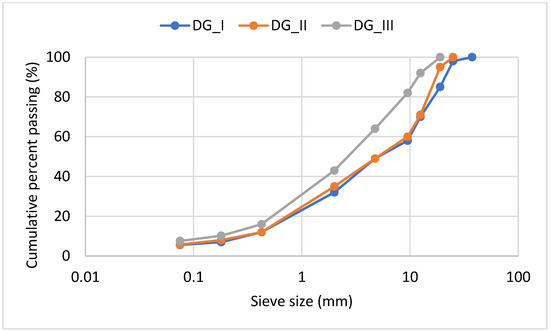
Figure 1.
Sieve analysis: Dense-graded (DG) mixtures.
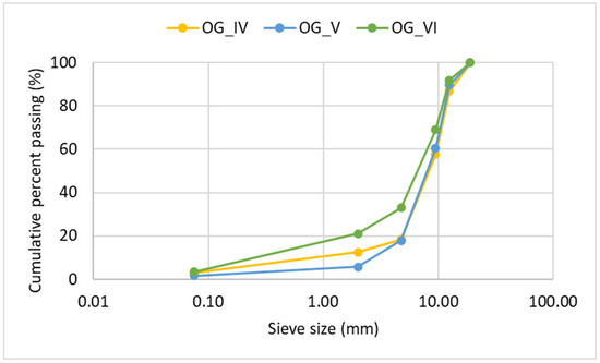
Figure 2.
Sieve analysis: Open-graded (OG) mixtures.
Prior to specimen compaction, the maximum theoretical specific gravity of each mixture was determined in the laboratory to enable accurate calculation of air void content. Compaction was carried out using a gyratory compactor, in accordance with EN 12697-31 [22]. Gyratory compaction is the standard method required for preparing specimens for dynamic modulus (E*) testing, as specified by AASHTO T 342-22 [23]. It is also the primary compaction method used in the development of widely adopted E* prediction models.
To achieve a range of air void contents, specimens were compacted to varying densities. Initially, each specimen was compacted to dimensions of 170 mm in height and 150 mm in diameter, as per standard specifications. Subsequently, the specimens were cored and cut to the final dimensions of 150 mm in height and 100 mm in diameter, following relevant standards.
In total, 36 specimens were compacted: 27 dense-graded (DG) specimens and 9 open-graded (OG) specimens. For each mixture and asphalt content, multiple specimens were prepared at different compaction levels to vary the air void content. Air voids for the DG specimens were determined using the saturated surface dry (SSD) method, while for the OG specimens, the dimensional method was applied, in line with EN 12697-06 [24] and EN 12697-08 [25]. Table 1 provides detailed information on the compacted specimens.

Table 1.
Volumetric composition of specimens.
2.2. Dielectric Constant Measurement
The dielectric constant of the asphalt mix specimens was measured using an open-ended coaxial probe integrated into the Percometer device. This non-destructive device operates at a frequency of 50 MHz, which restricts its penetration depth to approximately 3–5 cm from the surface, making it suitable for near-surface evaluations. Percometer measurements exhibit good repeatability under controlled conditions, while reproducibility across laboratories can be satisfactory if standardized equipment usage and rigorous adherence to a unified measurement protocol are maintained [26]. The device can measure various surface geometries by using appropriately shaped probes to ensure full contact between the probe and the specimen surface. In this study, two probe types were utilized: a flat-surfaced probe for measurements on the top and bottom faces of the specimens and a curved-surfaced probe for measurements along the cylindrical sides (Figure 3).
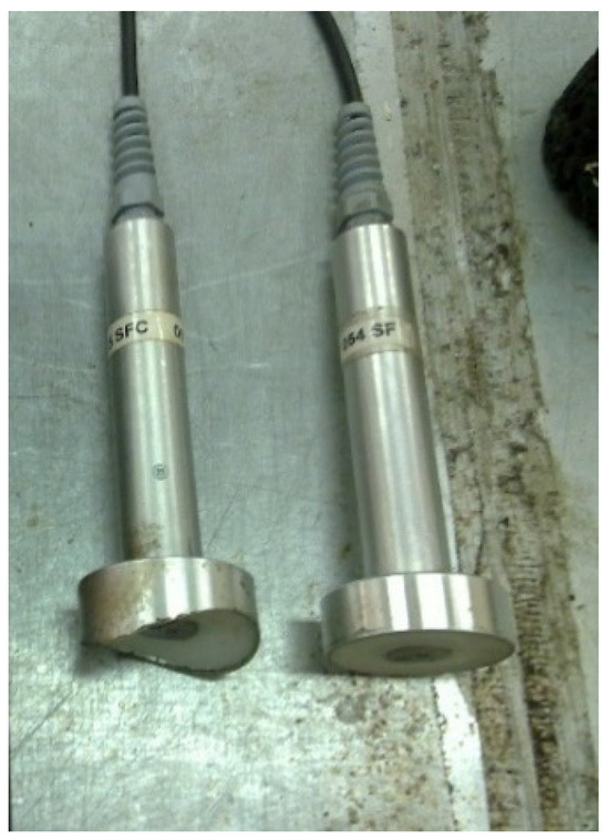
Figure 3.
Percometer probe types.
Dielectric measurements were taken at six evenly distributed locations on the top, six at the bottom and six along the side of each specimen, totaling eighteen readings per specimen.
2.3. Dynamic Modulus Measurement
The dynamic modulus (E*) for each HMA mixture was determined in accordance with AASHTO TP62 [27]. Specimens were subjected to a range of temperatures (from 4 °C to 37 °C) and loading frequencies (from 0.1 Hz to 25 Hz) to capture the typical traffic loading and environmental conditions experienced in pavements.
2.4. Dynamic Modulus Estimation
The dynamic modulus (E*) was estimated using predictive algorithms developed through the calibration of the NCHRP 1-37A model to a broader pool of local materials, which included mixtures with similar characteristics to those used in this study [10]. The general form of the equations is presented in Equation (1), while the values of the variable coefficients are provided in Table 2.
where Ε*: dynamic modulus of the mixture (psi), η: viscosity of the binder (106 poise), f: loading frequency (Hz), Va: air voids (% by volume), Vbeff: effective binder (% by volume), ρ34: cumulative percentage retained on a 3/4 inch (or 19 mm) sieve, ρ38: cumulative percentage retained on a 3/8 inch (or 9.5 mm) sieve, ρ4: cumulative percentage retained on No. 4 (or 4.75 mm) sieve, ρ200: percentage passing No. 200 (or 0.075 mm) sieve.
Table 2.
Variable coefficients of the E* predictive algorithms.
These predictive algorithms will be employed to investigate whether the dielectric constant can serve as an input parameter for estimating the dynamic modulus (E*) through a calibration process.
3. Data Analysis and Results
3.1. Dielectric Values
Minimal variation was observed between the dielectric constant values (εr) at the six points on each surface, as well as among the top and bottom readings of a given specimen. The standard deviation of the measured εr at the top and the bottom of the specimen was typically <0.1, while at the side of the specimen, it was <0.2. However, in some cases, the εr values measured along the sides of the specimens differed slightly from those recorded on the top and bottom surfaces (Figure 4 and Figure 5). This discrepancy may be attributed to factors such as minor compaction variability along the specimen height, slight differences in surface texture due to coring and cutting processes or challenges in achieving full and uniform contact between the curved probe and the side surface. Therefore, for further analysis, three εr values were considered for each specimen: the average of the top and bottom surface readings, the average of the side surface readings and the combined average of all measurements across all surfaces.
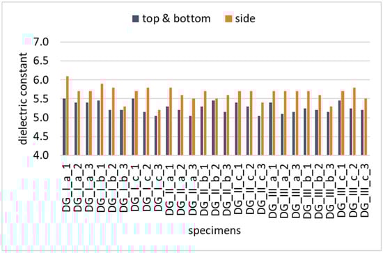
Figure 4.
Dielectric values of DG specimens.
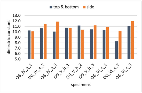
Figure 5.
Dielectric values of OG specimens.
Despite the fact that, according to the international literature, the dielectric constant and air void content are inversely related, the opposite trend was observed in this study between OG and DG mixes; namely, open-graded (OG) mixtures, which have higher air void content, exhibited higher dielectric constant values compared to dense-graded (DG) mixtures. This is attributed to the fact that OG mixes contain slag aggregates, which by nature are highly conductive. While OG mixtures containing slag aggregates exhibited higher dielectric constant values—attributed to the conductive nature of slag—the potential influence of slag heterogeneity on measurement variability was minimal. This is likely because all specimens were prepared and compacted under controlled laboratory conditions, ensuring good material homogeneity and minimizing localized inconsistencies. As such, any increased variability due to slag distribution was not significant within the scope of this study.
3.2. Relationship Between HMA Dielectric Value and Air Void and Binder Content
Since the dielectric constant of HMA specimens is influenced by air void content and binder distribution, their relationship was first examined in the initial stage of the analysis. Figure 6, Figure 7 and Figure 8 illustrate the correlation between air void content (Va) and the three dielectric constant (εr) values for DG mixes: the average of top and bottom (T&B) surface readings, the average of side readings (S) and the overall average across all surfaces (AVER). Figure 9, Figure 10 and Figure 11 present the correlation between the ratio Vbeff/(Vbeff + Va) and the three dielectric constant (εr) values for DG mixes. This ratio was selected for two main reasons: first, it incorporates parameters known to influence εr (i.e., binder content and air voids), and second, it is a variable in the E* predictive algorithms. Figure 12 and Figure 13 illustrate the corresponding correlations for the OG mixes, analogous to those presented earlier for the DG mixes. Table 3 presents the linear regression parameters and the coefficient of determination (R2).
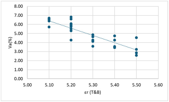
Figure 6.
Correlation between εr (top and bottom) and Va: DG mixes.
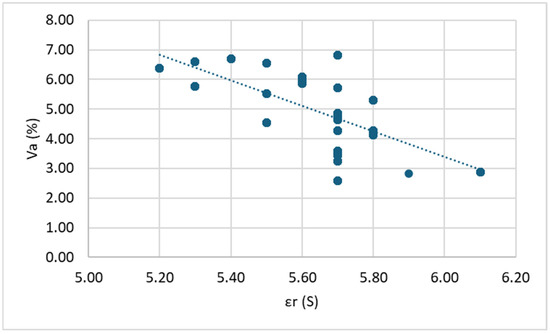
Figure 7.
Correlation between εr (side) and Va: DG mixes.
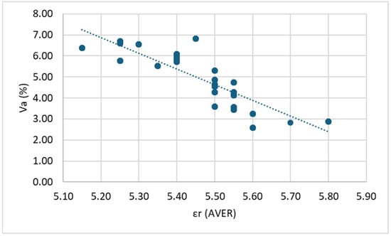
Figure 8.
Correlation between εr (total average) and Va: DG mixes.
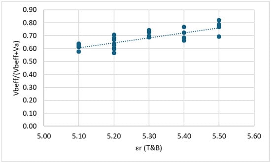
Figure 9.
Correlation between εr (top and bottom) and Vbeff/(Vbeff + Va): DG mixes.
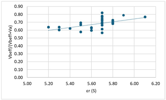
Figure 10.
Correlation between εr (side) and Vbeff/(Vbeff + Va): DG mixes.
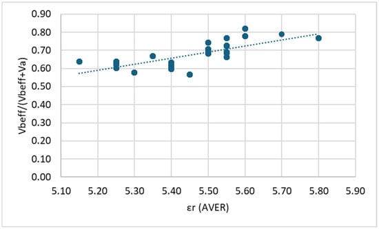
Figure 11.
Correlation between εr (total average) and Vbeff/(Vbeff + Va): DG mixes.
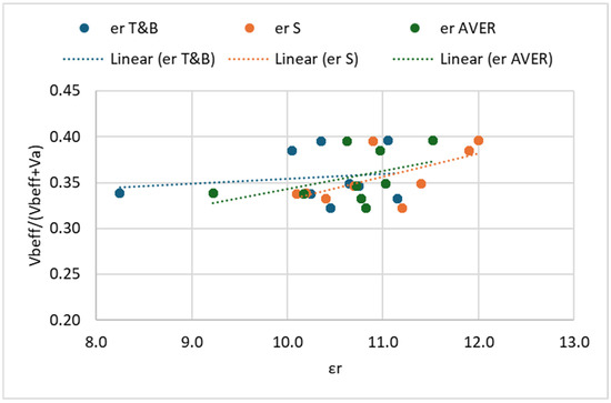
Figure 12.
Correlation between εr and Va: OG mixes.
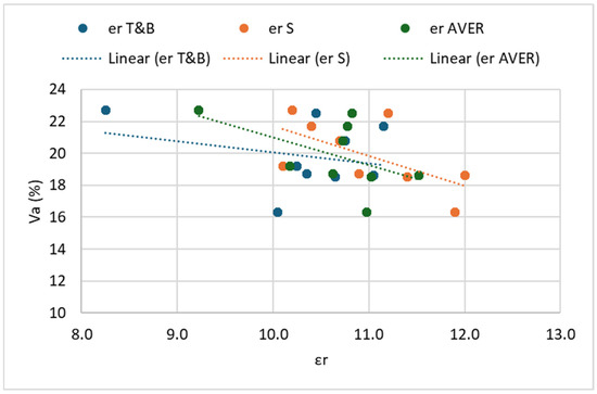
Figure 13.
Correlation between εr and Vbeff/(Vbeff + Va): OG mixes.
Table 3.
Regression parameters and goodness-of-fit metrics.
In all cases, it is observed that within each mix (DG and OG), as the dielectric constant (εr) increases, the air void content (Va) decreases. This observation aligns with the existing literature, which indicates that air, having a dielectric constant close to 1, reduces the overall dielectric constant of asphalt mixtures. Consequently, specimens with lower air void content exhibit higher εr values. On the other hand, a clear positive linear trend is observed between εr and the ratio Vbeff/(Vbeff + Va). This relationship is expected, as higher εr values are associated with reduced air voids and/or increased effective binder volume, both of which contribute to a higher ratio.
To evaluate the strength of these relationships, the coefficient of determination (R2) is considered. For dense-graded (DG) mixtures, a strong correlation is evident between Va and εr values measured at the top and bottom surfaces, as well as the total average. However, εr values obtained from side measurements show only a moderate correlation. Likewise, the correlation between Vbeff/(Vbeff + Va) and εr is moderate to weak when using side measurements.
In contrast, open-graded (OG) mixtures demonstrate weak correlations in all examined cases, likely due to their higher heterogeneity and increased interconnected void structure, which may affect both dielectric readings and volumetric consistency. Further, it is noted that the OG mixture dataset is relatively limited (three mixtures compared to nine DG mixtures), which may partly explain the weaker correlations observed for OG mixes. This limitation highlights the need for caution when interpreting and generalizing the results related to OG mixtures and suggests that further studies incorporating a larger number of OG mixtures are necessary to confirm these findings.
Considering the correlation between the specified volumetric parameters and the dielectric value, an effort was made to incorporate the dielectric value into the E* predictive algorithm instead of the volumetric parameters. Despite the poor correlation for OG mixes, the same procedure was followed.
3.3. Development of E* Predictive Algorithm
The general form of the model, derived from Equation (1) by replacing the variables Va and Vbeff/(Vbeff +Va) with the dielectric constant (εr), is presented in Equation (2).
Model development was carried out using non-linear optimization to estimate new variable coefficients, with convergence based on minimizing the sum of squared errors between measured and predicted E* values in logarithmic scale. In this process, three models were investigated, each incorporating a different dielectric input: the top and bottom εr values, the side εr value and the average of all εr measurements. Table 4 presents the SSE of the three models for DG mixes upon the optimization process.
Table 4.
SSE of E* predictive models.
It is observed that using the εr values recorded at the top and bottom of the specimens results in lower SSE values for DG mixes. For OG mixes, the SSE value when incorporating the side measurements of the εr is slightly lower than the one with the top and bottom εr values. Therefore, for validation and verification purposes, the predictive algorithm that incorporates the dielectric values recorded at the top and bottom of the specimen will be considered.
The values of the variable coefficients of the dielectric-based modulus estimation (DIME) algorithms developed are given in Table 5.
Table 5.
Variable coefficient values of the new algorithms.
The applicability of the DIME models was assessed using scatter plots comparing the measured dynamic modulus values (E*_lab) with the predicted values (E*_DIME), as shown in Figure 14 and Figure 15, for the DG and OG mixes, respectively. The line of equality is also included to evaluate the accuracy of the predictions.
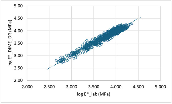
Figure 14.
Comparison of measured and predicted E* values: DG mixes.
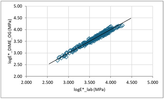
Figure 15.
Comparison of measured and predicted E* values: OG mixes.
To evaluate the adequacy and reliability of the DIME models, residual diagnostics were performed. These plots help identify the patterns, biases or heteroscedasticity in the model predictions (Figure 16 and Figure 17).
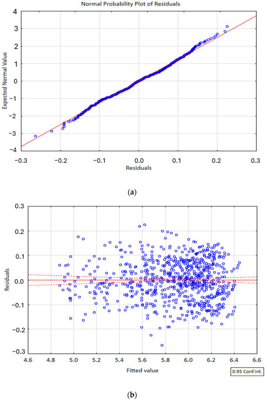
Figure 16.
Validation of the DIME algorithm for DG mixes (a) normal probability plot and (b) residuals versus fitted values.
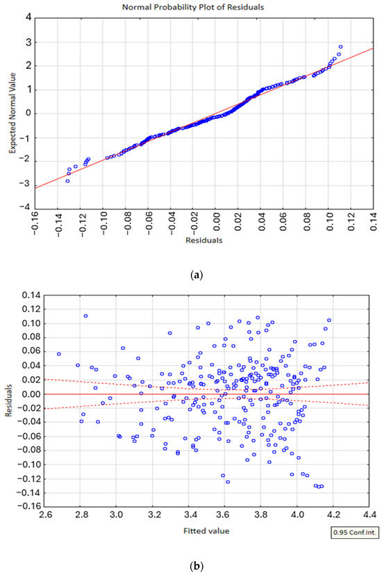
Figure 17.
Validation of the DIME algorithm for OG mixes (a) normal probability plot and (b) residuals versus fitted values.
The normal probability plot of the residuals (Figure 16a and Figure 17a) indicates that the residuals closely follow a straight line, suggesting that they are approximately normally distributed. This supports the assumption of normality, which is critical for the validity of regression-based modeling. Additionally, the residuals versus fitted values plot (Figure 16b and Figure 17b) shows a random scatter of points around the zero line, with no discernible pattern or systematic structure. This randomness implies that the variance of the residuals remains relatively constant across the range of fitted values, satisfying the assumption of homoscedasticity. Together, these results confirm that the model predictions are statistically sound and that the residuals do not exhibit any major violations of the underlying assumptions.
3.4. Model Verification
To assess the predictive accuracy of the developed DIME models, additional specimens were fabricated for laboratory measurement of both dynamic modulus (E*) and dielectric values, as well as model-based estimation of E*. A total of twelve specimens were prepared: nine DG and three OG mix specimens. Each specimen reflected the gradation and asphalt content of the original mixtures used during model development. The air void levels were controlled to remain within the range observed in the initial test specimens. Table 6 presents the air void content and the measured dielectric values (average value of the top and bottom of the specimen).
Table 6.
DG and OG mix specimens for the verification process.
Figure 18 and Figure 19 show the measured and predicted E* values along with the line of equality for DG and OG mixes, respectively. The SSE value for DG mixes is equal to 2.04, while for OG mixes, it is 1.04. The results of the unconstrained linear regression analysis revealed a slope of 0.9414 and an intercept of 0.1833 for the DG mixes, indicating a slight underestimation in the predicted values. For the OG mixes, the slope and intercept were found to be 0.9677 and 0.1948, respectively, suggesting a marginally improved agreement between the measured and predicted values compared to the DG mixes.
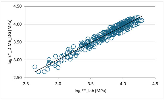
Figure 18.
Predicted (DIME model) versus measured E* values: DG mixes.
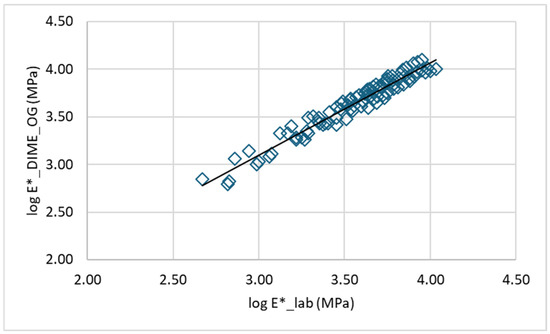
Figure 19.
Predicted (DIME model) versus measured E* values: OG mixes.
Overall, the findings highlight the effectiveness of the developed DIME models in estimating E*, offering a practical tool for reducing both the cost and time associated with establishing the dynamic modulus (E*) by minimizing the need for extensive laboratory testing while still maintaining acceptable levels of accuracy.
4. Conclusions
Based on the investigation and analysis conducted in this study, the following key conclusions can be drawn:
- Dielectric constant measurements at the top and bottom of the specimens are more homogeneous compared to the measured dielectric constant at the side of the specimens. This may be attributed to factors such as minor compaction variability along the specimen height, slight differences in surface texture due to coring and cutting processes or challenges in achieving full and uniform contact between the curved probe and the side surface.
- The dielectric constant values of open-graded mixes, which have higher air void content, exhibited higher dielectric constant values compared to dense-graded mixtures. This stands in contrast with the international literature but is attributed to the fact that open-graded mixes contain slag aggregates, which by nature are highly conductive.
- For dense-graded mixtures, a clear inverse relationship was observed between dielectric constant and air void content, consistent with findings in the literature. The correlation was weaker in open-graded mixtures, likely due to increased heterogeneity and the influence of conductive slag aggregates. Further, the weaker correlations observed for OG mixes could be attributed to the limited dataset. Therefore, further studies incorporating a larger number of OG mixtures are necessary to confirm these findings.
- Significant correlations were found between dielectric constant and the volumetric parameter Vbeff/(Vbeff +Va), particularly for DG mixes, indicating that εr reflects both air void and binder characteristics.
- Substituting volumetric variables with εr values (top and bottom of the specimen, side of the specimen and average of all measurements) led to the development of three predictive algorithms for each mix type. The model incorporating dielectric measurements from the top and bottom specimen surfaces exhibited the best performance. Therefore, two models were developed based on the proposed dielectric-based modulus estimation (DIME) approach: one tailored for dense-graded mixtures and another for open-graded mixtures.
- The weak correlations between ϵr and volumetric properties for OG mixtures may suggest limited predictive reliability of the DIME_OG model. Therefore, this model could be considered preliminary but forms a solid basis for further validation with a broader OG dataset.
- Verification using an independent set of DG and OG specimens yielded strong results, with regression slopes near unity and low SSE values, further validating the robustness of the proposed models.
- The use of dielectric measurements instead of extensive modulus testing presents a practical solution for pavement engineers, significantly reducing testing time and costs while maintaining reliable accuracy.
In summary, the DIME models developed in this research study confirm the viability of using dielectric constant as a surrogate input for E* estimation in flexible pavement design and rehabilitation, asphalt mix performance and pavement performance, particularly for dense-graded mixtures. The proposed approach offers a simplified framework toward this aim. Future work should focus on expanding the model to account for broader material types, environmental conditions and field validations.
Author Contributions
Conceptualization, K.G.; methodology, K.G.; software, K.G.; validation, K.G.; formal analysis, K.G.; investigation, K.G.; resources, A.L.; data curation, K.G.; writing—original draft preparation, K.G.; writing—review and editing, A.L. and K.G. All authors have read and agreed to the published version of the manuscript.
Funding
This research received no external funding.
Data Availability Statement
The original contributions presented in this study are included in the article. Further inquiries can be directed to the corresponding author.
Conflicts of Interest
The authors declare no conflicts of interest.
References
- Baltrušaitis, A.; Vaitkus, A.; Smirnovs, J. Asphalt Layer Density and Air Voids Content: GPR and Laboratory Testing Data Reliance. Balt. J. Road Bridge Eng. 2020, 15, 93–110. [Google Scholar] [CrossRef]
- Cao, Q.; Al-Qadi, I.L. Development of a Numerical Model to Predict the Dielectric Properties of Heterogeneous Asphalt Concrete. Sensors 2021, 21, 2643. [Google Scholar] [CrossRef]
- Chen, Y.; Li, F.; Zhou, S.; Zhang, X. Improved Density Prediction Model Based on Global Optimization Algorithm for GPR System. Measurement 2024, 237, 115243. [Google Scholar] [CrossRef]
- Abufares, L.; Al-Qadi, I.L. Development of Aggregate Dielectric Constant Database Protocol for Asphalt Concrete Density Prediction. Transp. Res. Rec. 2024, 2678, 376–388. [Google Scholar] [CrossRef]
- Georgouli, K.; Plati, C. Dielectric Response of Asphalt Mixtures and Relationship to Air Voids and Stiffness. Constr. Mater. 2024, 4, 566–580. [Google Scholar] [CrossRef]
- Cao, Q.; Al-Qadi, I.L. Effect of Moisture Content on Calculated Dielectric Properties of Asphalt Concrete Pavements from Ground-Penetrating Radar Measurements. Remote. Sens. 2022, 14, 34. [Google Scholar] [CrossRef]
- Steiner, T.; Hoegh, K.; Teshale, E.Z.; Dai, S. Method for Assessment of Modeling Quality for Asphalt Dielectric Constant to Density Calibration. J. Transp. Eng. Part B Pavements 2020, 146, 04020054. [Google Scholar] [CrossRef]
- Primusz, P.; Abdelsamei, E.; Ali, A.M.; Sipos, G.; Fi, I.; Herceg, A.; Tóth, C. Assessment of In Situ Compactness and Air Void Content of New Asphalt Layers Using Ground-Penetrating Radar Measurements. Appl. Sci. 2024, 14, 614. [Google Scholar] [CrossRef]
- Liu, Q.; Lu, J.; Zhang, Z.; Chen, Z.; Wang, T.; Zheng, Q. Comprehensive Study on Dynamic Modulus and Road Performance of High-Performance Asphalt Mixture. Buildings 2024, 14, 3643. [Google Scholar] [CrossRef]
- Georgouli, K.; Loizos, A.; Plati, C. Calibration of Dynamic Modulus Predictive Model. Constr. Build. Mater. 2016, 102, 65–75. [Google Scholar] [CrossRef]
- Solatifar, N. Performance Evaluation of Dynamic Modulus Predictive Models for Asphalt Mixtures. J. Rehabil. Civ. Eng. 2020, 8, 87–97. [Google Scholar] [CrossRef]
- Zhang, D.; Birgisson, B.; Luo, X. A New Dynamic Modulus Predictive Model for Asphalt Mixtures Based on the Law of Mixtures. Constr. Build. Mater. 2020, 255, 119348. [Google Scholar] [CrossRef]
- Gong, H.; Sun, Y.; Dong, Y.; Han, B.; Polaczyk, P.; Hu, W.; Huang, B. Improved Estimation of Dynamic Modulus for Hot Mix Asphalt Using Deep Learning. Constr. Build. Mater. 2020, 263, 119912. [Google Scholar] [CrossRef]
- Golafshani, E.M.; Behnood, A.; Karimi, M.M. Predicting the Dynamic Modulus of Asphalt Mixture Using Hybridized Artificial Neural Network and Grey Wolf Optimizer. Int. J. Pavement Eng. 2021, 24, 2005056. [Google Scholar] [CrossRef]
- Al-Tawalbeh, A.; Sirin, O.; Sadeq, M.; Sebaaly, H.; Masad, E. Evaluation and Calibration of Dynamic Modulus Prediction Models of Asphalt Mixtures for Hot Climates: Qatar as a Case Study. Case Stud. Constr. Mater. 2022, 17, e01580. [Google Scholar] [CrossRef]
- Xu, W.; Huang, X.; Yang, Z.; Zhou, M.; Huang, J. Developing Hybrid Machine Learning Models to Determine the Dynamic Modulus (E*) of Asphalt Mixtures Using Parameters in Witczak 1-40D Model: A Comparative Study. Materials 2022, 15, 1791. [Google Scholar] [CrossRef]
- Worthey, H.; Yang, J.J.; Kim, S.S. Tree-Based Ensemble Methods: Predicting Asphalt Mixture Dynamic Modulus for Flexible Pavement Design. KSCE J. Civ. Eng. 2021, 25, 4231–4239. [Google Scholar] [CrossRef]
- Aidara, M.L.C.; Ba, M.; Carter, A. Development of a Dynamic Modulus Prediction Model for Hot Mixture Asphalt and Study of the Impact of Aggregate Type and Its Electrochemical Properties. Open J. Civ. Eng. 2020, 10, 213–225. [Google Scholar] [CrossRef]
- Moussa, G.S.; Owais, M. Pre-Trained Deep Learning for Hot-Mix Asphalt Dynamic Modulus Prediction with Laboratory Effort Reduction. Constr. Build. Mater. 2020, 265, 120239. [Google Scholar] [CrossRef]
- Chen, F.; Balieu, R. A State-of-the-Art Review of Intrinsic and Enhanced Electrical Properties of Asphalt Materials: Theories, Analyses and Applications. Mater. Des. 2020, 195, 109067. [Google Scholar] [CrossRef]
- Cui, L.; Ling, T.; Sun, F.; Zhang, Z.; Xin, J. Study of In Situ Dynamic Modulus Prediction of Asphalt Mixture Utilizing Ground-Penetrating Radar Technology. Constr. Build. Mater. 2022, 350, 128695. [Google Scholar] [CrossRef]
- EN 12697-31; Bituminous Mixtures—Test Methods—Part 31: Specimen Preparation by Gyratory Compactor. European Committee for Standardization: Brussels, Belgium, 2019.
- AASHTO T 342-22; Standard Method of Test for Determining Dynamic Modulus of Hot Mix Asphalt (HMA). American Association of State Highway and Transportation Officials: Washington, DC, USA, 2022.
- EN 12697-6; Bituminous Mixtures—Test Methods—Part 6: Determination of Bulk Density of Bituminous Specimens. European Committee for Standardization: Brussels, Belgium, 2020.
- EN 12697-08; Bituminous Mixtures-Test Methods-Part 8: Determination of Void Characteristics of Bituminous Specimens. European Standard: Brussel, Belgium, 2019.
- Barbu, B.G.; Scullion, T. Repeatability and Reproducibility Study for Tube Suction Test; Report FHWA/TX-06/5-4114-01-1; Texas Transportation Institute, The Texas A&M University System College Station: College Station, TX, USA, 2005. [Google Scholar]
- AASHTO TP 62; Standard Method of Test for Determining Dynamic Modulus of Hot Mix Asphalt (HMA). American Association of State Highway and Transportation Officials: Washington, DC, USA, 2007.
Disclaimer/Publisher’s Note: The statements, opinions and data contained in all publications are solely those of the individual author(s) and contributor(s) and not of MDPI and/or the editor(s). MDPI and/or the editor(s) disclaim responsibility for any injury to people or property resulting from any ideas, methods, instructions or products referred to in the content. |
© 2025 by the authors. Licensee MDPI, Basel, Switzerland. This article is an open access article distributed under the terms and conditions of the Creative Commons Attribution (CC BY) license (https://creativecommons.org/licenses/by/4.0/).