1. Introduction
It is widely recognized that accurate characterization of unbound granular materials (UGMs) and subgrade soils is essential for effective pavement design and rehabilitation. The implementation of the modern Mechanistic–Empirical Pavement Design Guide (MEPDG) requires accurate modulus parameters for each unbound pavement layer [
1]. Resilient modulus (Mr), derived from the repeated load triaxial (RLT) test, is a fundamental engineering property used to define the stress–strain relationships of UGMs and subgrade under cyclic loading. Recently, with the advent of mechanistic–empirical pavement design procedures, various field modulus evaluation devices, such as the RLT, LWD, soil stiffness gauge (SSG) and dynamic cone penetrometer (DCP), have been developed and employed to assess the bearing capacity and modulus of UGMs and subgrade soils [
2,
3]. However, the use of stiffness moduli from devices other than the elastic modulus from the RLT test as input stiffness parameters for UGMs and subgrade soils in the MEPD software warrants further investigation. In addition, understanding the effect of using these stiffness moduli from devices other than the RLT test on the induced stresses and strains at critical points within the pavement structure as determined by the MEPD software requires further investigation, a focus of this study.
This study investigates variations in crucial stresses and strains within pavement structures when employing modulus data from repeated in-situ lightweight deflectometer (LWD) tests instead of the corresponding Mr data from repeated load triaxial (RLT) tests, conducted under similar conditions. These modulus values are pivotal inputs in the ERAPAVE Mechanistic–Empirical Pavement Design Guide utilized in Sweden. The study commences by elucidating the measurement processes for deformation and stiffness moduli, determined, respectively, by repeated LWD and RLT tests. The mathematical resilient modulus model, commonly employed in the Mechanistic–Empirical Pavement Design Guide (MEPDG), is also discussed. Critical locations for hot mix asphalt (HMA) pavement response, crucial in Swedish pavement design, are identified. The methodology for field and laboratory testing, along with the properties of the selected testing materials, is detailed. The impact of substituting RLT stiffness moduli with LWD deformation moduli on response measurements through ERAPAVE is thoroughly explored, and the outcomes are comprehensively discussed.
1.1. Repeated Lightweight Deflectometer (RLWD) Test
One notable advancement in assessing layer properties is the lightweight deflectometer (LWD), gaining popularity due to the success of its predecessor, the falling weight deflectometer [
1]. LWD offers a rapid, cost-effective, and nondestructive method for evaluating the structural adequacy of compacted road materials, setting it apart from other devices [
4,
5,
6].
The LWD determines the modulus by releasing a falling weight from a specific height onto its loading plate, measuring the maximum settlement. A velocity sensor or accelerometer records the velocity or acceleration of the plate or ground surface, depending on the sensor’s position. The type and position of the deflection sensor may vary among LWD devices. The in situ elastic modulus (Evd) is then determined by utilizing the measured applied load and center surface deflection, assuming a circular plate on a semi-infinite, isotropic and homogeneous half-space (Boussinesq solution).
Evd, also known as the deformation modulus, is a significant indicator of ground stiffness. Standard testing entails performing six drops to complete one test, with the first three drops aligning the loading plate correctly, and the latter three measuring the settlement. Evd is calculated using the average of the last three settlement measurements. Kuttah [
7] emphasized an advancement involving an upgraded LWD version, involving the use of a newly manufactured LWD with a higher number of repeated drops compared to traditional LWD tests. This modification provides elastic moduli closer to stiffness moduli obtained under similar testing conditions in RLT tests for sandy and granular base materials.
The innovation in this improved LWD variant centers on the incorporation of a control beam furnished with two linear variable differential transformers (LVDTs), enabling the recording of plastic deformations during testing. This progress allows for ongoing monitoring and graphical representation of the load versus accumulated soil deformation loops, mirroring the stress–strain loops typically recorded in RLT tests. This feature streamlines the immediate determination of the required number of drops (cycles) during the LWD test to bring the soil as close to its elastic state as possible. At these specific load repetitions, the elastic moduli are measured and employed as Evd values in the ongoing study.
The calculation of Evd employs the elastic half-space theory. Previous studies [
8,
9,
10] have extensively discussed LWD theory and measured moduli, although these specifics are not within the scope of this paper. Equation (1) provides the modulus of elasticity calculation for a single-layer system, based on Boussinesq’s [
11] theory. This equation assumes that the test medium behaves as a linearly elastic, isotropic, and homogeneous semi-infinite continuum.
Here, Evd represents the modulus of elasticity, determined dynamically through field LWD tests. The symbol ‘k’ denotes soil stiffness, computed as F/δ by the LWD device, where δ signifies peak deformation and F represents the peak impact load or maximum applied axial load. ‘r
0 represents the plate radius, while ‘ν’ stands for Poisson’s ratio. The parameter ‘A’ denotes the stress distribution factor, taking the value of 4 for cohesive soil and 3π/4 for noncohesive soil [
12].
Please be aware that nearly all existing LWD software includes the Evd equation, generating it as the resulting value. However, Afsharikia [
13] provides specific information regarding the derivation of Equation (1) and its utilization for determining the dynamic deformation modulus through LWD testing.
1.2. Repeated Load Triaxial (RLT) Test
Resilient modulus (Mr) is a key engineering property describing the stress–strain relationship of soil/unbound granular materials (UGMs) under cyclic loading. Typically, laboratory methods for determining modulus of elasticity are based on a repeated loading triaxial test. During cyclic loading, unbound materials exhibit elastoplastic behavior characterized by increases in stiffness (resilient modulus) and permanent deformation with load repetitions of Haversine loading pulses. Mathematically, it is the ratio of the deviatoric stress to the elastic or recoverable strain after a significant number of load cycles, as expressed in Equation (2):
The aim of laboratory testing is to simulate field conditions, so factors such as water content, soil type and sample condition must be taken into account. The resilient modulus of the subgrade depends primarily on three factors: (1) stress state; (2) soil type and structure; and (3) soil physical properties. Numerous researchers, such as Oh et al. [
14], Han and Vanapalli [
15], Abu-Farsakh et al. [
16], have observed that subgrade resilient modulus is significantly affected by deviatoric stress, density and moisture content, especially in fine-grained soils. The effect of confinement on resilient modulus values varies depending on the type of material and its properties [
17].
2. Resilient Modulus Models for MEPDG
Moossazadeh and Witczak [
10] proposed the resilient modulus model that has deviator stress as the only attribute of the model.
where σ
d is the deviator stress and k
1 and k
2 are constants dependent on material type and soil physical properties.
Equation (4) can also be represented in non-dimensional form as follows:
where P
a is the reference pressure of 100 kPa introduced to express the coefficients in non-dimensional form and σ
d = F/A, where F = axial applied force/area.
Seed et al. [
18] suggested that the resilient modulus is a function of the sum of principal stresses or the bulk stress (first invariant of stress) and the relation between resilient modulus and bulk stress can be expressed as a straight line in a log–log scale. The model can be expressed in the following form:
where Mr = resilient modulus; θ = first stress invariant (bulk stress) = σ
1 + σ
2 + σ
3; k
1, k
2 = constants depending on material properties.
Equation (6) can also be represented in non-dimensional form as follows:
where P
a is the reference pressure of 100 kPa introduced to express the coefficients in non-dimensional form. This equation is generally known as a widely used K-θ model and is supported by the data obtained from repeated load triaxial tests. The simplicity of the K-θ model has made it extremely useful and widely accepted for analysis of stress dependence of material stiffness [
19,
20,
21,
22,
23].
Equation (6) was incorporated in the MEPDG with adding one to the shear stress term and it is well-known as the universal Witczak model.
The model for Mr implemented in the mechanistic–empirical AASHTO Guide and ERAPAVE for the Design of New and Rehabilitated Pavement Structures is used for fine and granular soils. This model is defined as
where Mr = resilient modulus;
octahedral shear stress; θ = bulk stress; P
a = atmospheric pressure; k
1, k
2 and k
3 are model parameters.
For simplicity, usually k3 is considered zero, and the simple form given in Equation (6) is usually adopted.
The current study emphasizes Equation (6), chosen for its widespread use in mechanistic–empirical pavement design, to provide a basis for meaningful comparisons. In addition, Equation (4) is strategically used to bridge the gap between the LWD and RLT datasets, emphasizing its key role as a link in this comparative analysis.
To determine the stress–strain relationship experimentally, and hence k
1, k
2 and v, a number of measurements are required to cover the actual range of mean stresses p and deviatoric stresses q caused by different weights of traffic axle loads. The RLT test method can be used for this estimation where different stress paths are applied [
24].
In the field of flexible pavements, a fundamental approach to mathematically modeling the pavement structure is layered elastic analysis. This method involves defining material layer parameters such as Young’s modulus, Poisson’s ratio and layer thickness. Each layer is assumed to be infinite in the horizontal direction, while the subgrade is assumed to be infinite in the downward direction. These defined material parameters, coupled with the given loading conditions, facilitate the calculation of stresses, strains and pavement deflections.
Using computer programs based on layered elastic analysis, the theoretical stresses, strains and deflections can be calculated at any point within the pavement structure.
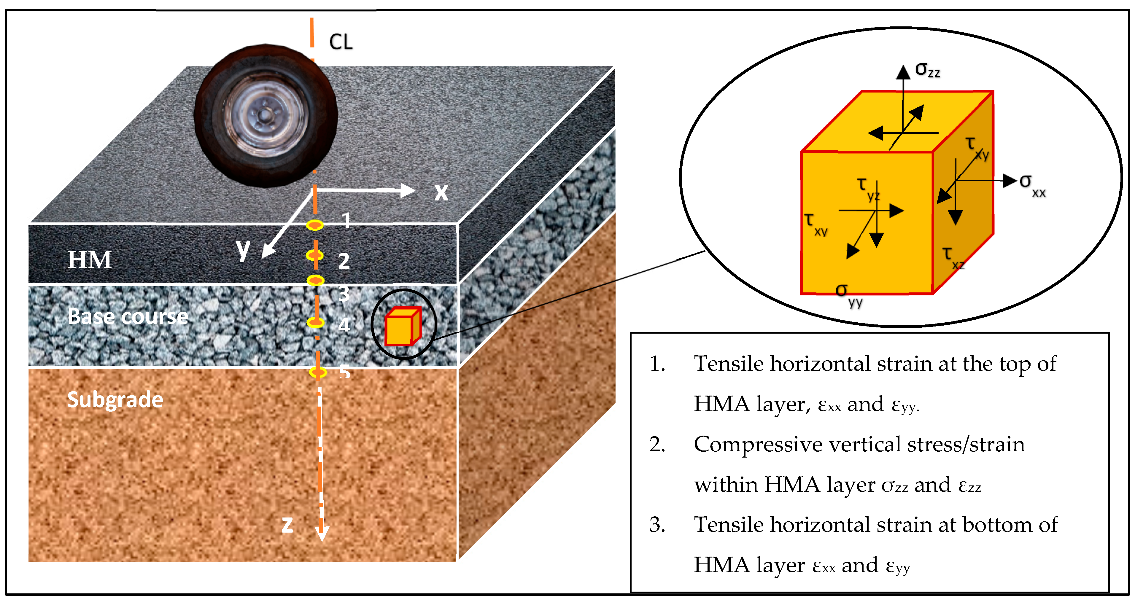
Figure 1 provides a visual representation of the critical locations for hot mix asphalt (HMA) pavement response.
These critical response locations provide insight into various aspects of pavement analysis. Horizontal tensile strain at the top and bottom of the asphalt concrete (AC) layer is critical in assessing fatigue cracking. Compressive vertical stress/strain within the HMA layer is important in determining rutting in this layer. In addition, rutting in the base and sub-base layers is assessed by their respective compressive vertical stress/strain. Finally, to predict rutting failure in the subgrade, emphasis is placed on analyzing the vertical compressive stress/strain at the top of the subgrade.
3. Testing Methodology
The testing approach involved conducting in situ repeated lightweight deflectometer (LWD) tests and repeated load triaxial (RLT) tests under similar LWD testing conditions. The objective was to determine the deformation modulus (Evd) through LWD tests and the corresponding resilient modulus (Mr) from RLT tests for three distinct types of road construction materials: base course material, sandy subgrade soil, and silty sand subgrade soil.
All the data obtained from the in situ LWD tests and the laboratory RLT tests were used in Excel software to calculate the constants k1 and k2 as defined in Equations (4) and (6). These equations were used to derive stiffness moduli from the RLT tests and deformation moduli from the in situ LWD tests. The determined k1 and k2 values were then input into the ERAPAVE software to evaluate the critical stresses and strains within the pavement structure.
Finally, the response measurements obtained by ERAPAVE were compared to identify variations resulting from the different approaches and models used to determine the k1 and k2 constants. These approaches included RLT testing and LWD testing using the models described in Equations (4) and (6).
3.1. In Situ Testing Plan and Equipment Used
In situ repeated lightweight deflectometer testing was used in the current research to determine the deflection moduli of the tested materials; see
Figure 2.
During the LWD test, the center-to-center deflection of the tested material surface was measured through holes in the loading plate by a high-precision seismic transducer (geophone). The plates used in this study were 20 cm and 30 cm in diameter.
In addition to LWD testing, the nuclear density gauge (NDG) was employed to determine the in situ density and moisture content of the tested soil within the test pit, following the methodology outlined by TDOK 0140 [
25]. The measurement process is applicable to materials with a diameter less than 125 mm. For tests conducted on clay, a maximum probe length of 30 cm was used, while for base course tests, a 20 cm probe length was utilized. Note that the NDG measurements were conducted immediately after the completion of LWD tests to ensure that the holes created by NDGs did not interfere with the LWD testing procedure.
Three types of commonly available materials were selected to test the possible use of the RLWD test to predict the response of flexible pavements, namely unbound granular material, sand and silty sand. The unbound granular material is normally used as a base and sub-base layer and the sand and silty sand materials are normally used as a sub-base layer. The selected base course material met the requirements of the Swedish standard for unbound materials used in road construction in Sweden according to TRVKB 10 [
26].
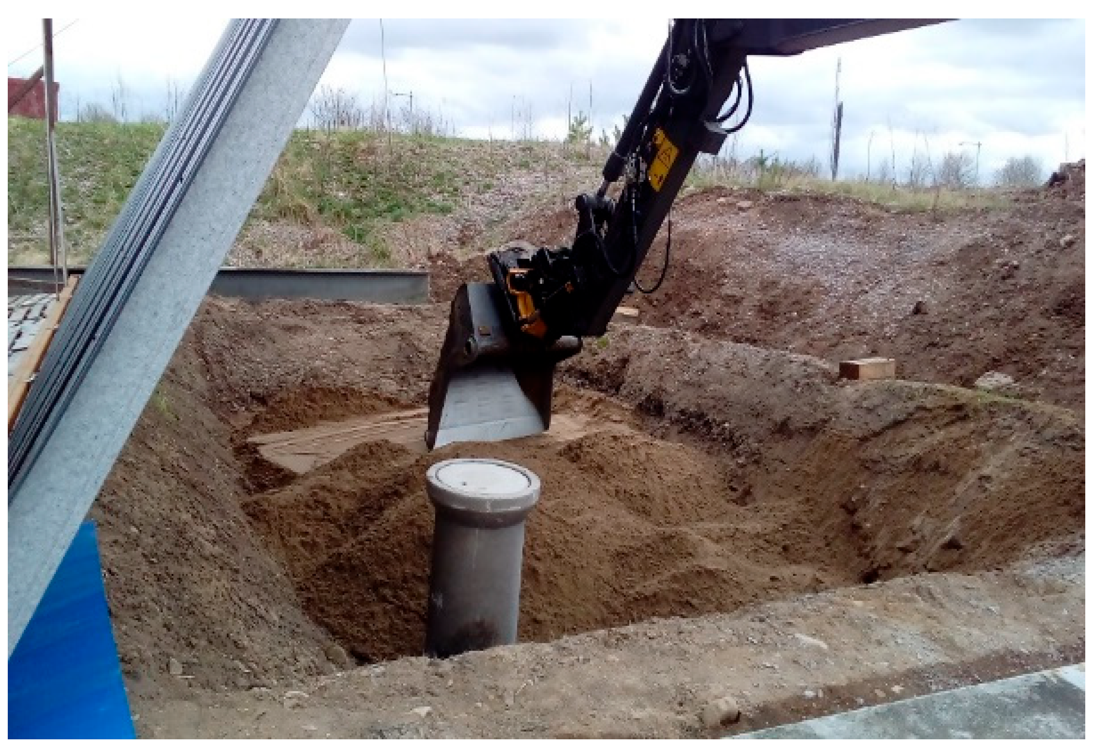
The test procedure for each material consisted of two phases. In the first phase, field tests were carried out in a large test pit containing the compacted material under controlled conditions. These field tests included lightweight deflectometer (LWD) evaluations, as well as field density and moisture content measurements.
The in situ LWD tests were carried out in a controlled environment within the test pit. The dimensions of the test pit were approximately 10 m long, 5 m wide and 1.5 m deep. The pit was equipped with a concrete well containing a water-discharging motor to facilitate the regulation of groundwater levels during testing. In addition, the test pit was equipped with an electrically operated roof panel that could be opened and closed by an electric motor, providing some control over the test conditions within the pit, as shown in
Figure 3.
Following the compaction of the target material using a small vibrator, specific points on the final compacted surface were marked with circles, indicating the chosen locations for testing with the lightweight deflectometer (LWD).
Table 1 provides an overview of the tests conducted on the base material within the test pit, presenting the respective details of the testing points along with the prevailing moisture content conditions.
For the sandy subgrade, the LWD tests were carried out at different water contents ranging from 3% to 9% according to NDG measurements. Within this range of water contents, the LWD tests were carried out at three different applied stress levels, namely about 45 kPa, 72 kPa and 100 kPa; see
Table 2.
When all the subgrade tests were completed, the compacted soil was excavated, and the pit refilled with the silty sand for further testing.
Table 3 gives a summary of the stresses applied using LWD on the silty sand subgrade tested for each point. The tests were carried out using a 200 mm diameter steel plate and simultaneous water content measurements were made using NDG tests.
The tested points were divided into two groups based on their proximity in time of testing and water content (W). Each group, as shown in
Table 3, contains three subgroups of points tested at target stresses of 50 kPa, 100 kPa and 200 kPa.
In addition,
Table 3 shows the degree of saturation and relative compaction values obtained during the repeated LWD measurements for the tested points.
3.2. Laboratory Testing Plan and Equipment Used
In the second phase, many laboratory tests were carried out on the same materials used in the field tests, including the material characterization tests and the repeated loading triaxial test. A series of laboratory tests were carried out on the selected soil to determine its physical properties, namely grain size distribution, clay fraction, soil classification, specific gravity, liquid and plastic limits and compaction characteristics.
The dynamic triaxial test was used in the current study to determine Young’s moduli of the three selected test materials under test conditions as similar as possible to those encountered during in situ LWD testing. The dynamic triaxial test is a laboratory method of simulating traffic loading on a material. A cylindrical specimen of unbound material is loaded in three dimensions. The specimen (with a diameter/height ratio of ½) is packed to the required specifications, density packing ratio and water content, often in relation to results from standardized laboratory packing methods.
The finished sample is fitted with steel end plates and a rubber membrane around the sample; see
Figure 4. The specimen is placed vertically in a pressure chamber. The chamber is pressurized in three dimensions, radially and axially, i.e., horizontally and vertically. In this study, this pressure is generated by compressed air and kept constant (CCP) in each load case. The chamber pressure is intended to simulate the support and pressure of the surrounding material.
In addition to the chamber pressure (a contact pressure to ensure that the beam is always against the specimen), the specimen can be subjected to a static axial load, also known as the minimum (min.) deviator stress. The test then proceeds by subjecting the specimen to a specified number of load cases with a specified number of pulses. A load case consists of a chamber pressure, an additional static axial load and a dynamic axial load at a specified frequency. The dynamic load consists of a sinusoidal load pulse. The dynamic load plus the static load is called the maximum (max.) deflection stress [
27]. The European standard has a method for determining only the stiffness modulus with two different levels, high and low. In this study, SS-EN 13286-7 [
28] was followed to determine the high-level stiffness modulus.
In the current study, the conditioning of each specimen was carried out for 2500 cycles with a constant confining pressure of 50 kPa and a deviator stress of 100 kPa.
The axial deformations of the specimen were measured using three linear variable differential transformers (LVDTs). These were mounted on the middle third of the specimen, maintaining an angle of 120° between them.
4. Characteristics of Test Materials
As mentioned above, three types of road construction materials were used in this study, namely 0–32 mm base course material, sandy sub-base and silty sand sub-base. The characteristics of each test material are discussed in the following paragraphs.
4.1. Unbound Base Material
For the granular sub-base, a 0/32 gravel material was selected for testing in this study. The gradation of the tested base material is shown in
Table 4 with the percentage pass and limits according to [
29].
The specific gravity of the selected base material was tested according to [
30] and found to be 2.72.
The compaction properties of the selected base material were determined by the modified Proctor test according to [
31]. The test was carried out by compacting several California Bearing Ratio (CBR) soil samples using a cylindrical mold with a diameter of 152.4 mm.
The results of the compaction tests showed that the compaction curve of the tested material is a one and a half peak curve with two optimum water contents and two maximum dry densities. One of the maximum dry densities is on the dry side (at W = 0%) and the other is on the wet side (around W = 6%). The maximum dry densities are 2.2 g/cm3 and 2.3 g/cm3 at 0% and 5.7% water content, respectively.
4.2. Sandy Subgrade Soil
A sandy subgrade soil has been selected to be tested in this study. The particle size distribution of the tested soil is illustrated in
Table 5 below:
According to VVTK Väg [
32], the tested soil is material type 2 (Hazard class 1), and according to SGF 81, it is a sediment sand.
The specific gravity of the selected sandy soil was tested according to Chapter G, and was found to be 2.664 mg/m3.
In this test, the compaction properties were determined by the modified Proctor test according to [
31]. The test was performed by compacting several CBR soil samples using a cylindrical mold with a diameter of 152.4 mm. The results of the compaction tests showed that the compaction curve of the tested soil is a one-and-a-half-peak curve with two optimum water contents and two maximum dry densities. One of the maximum dry densities is on the dry side (at W = 0%) and the other is on the wet side (at about W = 12%). The maximum dry densities are 1.8 and 1.72 g/cm
3 at 0 and 12% water content, respectively.
4.3. Silty Sand Subgrade Soil
As mentioned above, a silty sand subsoil was selected for testing in this study. The particle size distribution test on the selected soil was carried out, and the results of the test are presented in
Table 6 below:
The clay content of the soil was tested according to the VTI method for grain size distribution analysis with laser diffraction [10 nm–2 mm] and was found to be 5%.
According to VVTK Väg [
32], the tested soil is of material type 4A (mixed-grained soils with frost hazard class 3). According to [
33], the soil is classified as silty sand with 5% clay. The specific gravity of the selected soil was tested according to [
30], and found to be 2.64.
The liquid and plastic limits were determined at SGI (The Swedish Geotechnical Institute) according to [
34]. The test results showed a liquid limit (LL) of 18% and a plastic limit (PL) of 14.3%, resulting in a plasticity index of 3.7% for the tested soil.
In this project, compaction properties were determined using the modified Proctor test according to [
31]. The test was performed by compacting several soil samples using a cylindrical mold with a diameter of 152.4 mm. The soil samples were compacted at different mold water contents ranging from 0 to 16% to determine the water-density relationship.
The results of the compaction tests showed that the tested soil has a maximum dry density of 2.03 g/cm3 at an optimum moisture content of about 8.2%.
5. Results and Discussions
As mentioned above, the problem solver in Excel was used to determine k1 and k2 given in Equations (4) and (6) for the stiffness moduli obtained from the RLT tests and Equation (4) for the deformation moduli obtained from the in situ repeated LWD test. These k1 and k2 data were used in ERAPAVE to determine the critical stresses and strains within the pavement structure. Note that for all the cases studied, ko, the earth pressure coefficient, is assumed to be 0.53.
Furthermore, for all the cases studied, the traffic load and the output of the ERAPAVE program in terms of critical response locations were as shown in
Table 7 and
Table 8, respectively for all the cases studied. Regarding the selected critical response locations, the chosen locations are similar to those discussed previously and shown in
Figure 1, except for position 1, which is not usually considered as a steering response in road design in Sweden.
5.1. Observations in a Body of Unbound Base Material
Table 9 below shows the profile of the hypothetical pavement structure used to determine the response measurement when the base course is considered as a stress-sensitive layer in the ERAPAVE program.
5.1.1. For Unbound Base Layer Compacted at 3% Water Content
The use of the problem solver to calculate the function constants k
1 and k
2 used in Equations (4) and (6) based on the moduli determined from the repeated LWD and RLT tests has resulted in the constant values shown in
Table 10 for the three selected cases considered in this study together with the corresponding predicted layer moduli, i.e., k
1 and k
2 based on RLT test results and the prediction model given in Equation (4) and k
1 and k
2 based on RLT test results and the prediction model given in Equation (6); k
1 and k
2 based on RLT test results and the prediction model given in Equation (4); and k
1 and k
2 based on repeated LWD test results and the prediction model given in Equation (4).
From
Table 10, it can be seen that the input data in terms of k
1 and k
2 from Equation (6) and Equation (4) for the RLT test have resulted in Young’s moduli of 134.4 kPa and 248.3 kPa, respectively, (i.e., with approximately 59% difference between the two assumed models given in Equations (4) and (6) based on the same RLT test data).
When comparing the stiffness moduli calculated from Equation (4) using RLT data with those derived from the same equation using LWD data, a difference of approximately 12% was observed. This indicates that the use of LWD resulted in a smaller percentage difference in the stiffness moduli (Mr) calculated within ERAPAVE, in contrast to the larger difference seen when using two different models based on the same RLT test data.
Figure 5 shows the effect of the calculated coefficients k
1 and k
2 from different tests and models, as given in
Table 10, on the response measurements at four critical positions within the pavement structure as defined in
Figure 1.
Figure 5 illustrates slight variations in the recorded stresses and strains at the critical positions indicated in
Figure 1 for the various models (equations) adopted. However, a notable exception is observed in the case of the vertical compressive strain within the base/sub-base layer. For this strain, the model presented in Equation (6) showed a significantly higher value compared to the corresponding strains obtained by applying the model in Equation (4), for both RLT and LWD data.
This observation is probably due to the different predictive capabilities and assumptions of the models represented by Equations (4) and (6). These two equations have different underlying assumptions about the behavior of the base/sub-base layer that could lead to variations in the predicted vertical compressive strain. It is possible that the models have different sensitivities to water content. Equation (6) may be more sensitive to water content, resulting in lower measured stiffness moduli. This sensitivity results in a significant increase in predicted compressive strain, especially when compared to values derived from Equation (4) using LWD and RLT data. In addition, the behavior of the base/sub-base layer may be influenced by interactions with adjacent layers (e.g., surface layer, subgrade). Models may differ in how they account for these interactions.
5.1.2. For Unbound Base Layer Compacted at 6% Water Content
Similarly, to the case of the unbound base layer compacted at 3% water content,
Table 11 shows k
1 and k
2 used in Equations (4) and (6) for the three selected cases considered in this study, together with the corresponding predicted layer moduli for the case of the unbound base layer compacted at 6% water content.
It can be seen from
Table 11 that the input data in terms of k
1 and k
2 from Equation (6) and Equation (4) for the RLT test have resulted in stiffness moduli of 213.57 kPa and 371.56 kPa, respectively (i.e., with approximately 54% current difference between the two assumed models given in Equations (4) and (6) based on the same RLT test data).
For the case of 6% compacted base material, comparing the Mr calculated from Equation (4) based on LWD data with the corresponding moduli calculated from Equations (6) and (4) based on RLT data, the percentage difference was found to be approximately 5.6% and 59%, respectively. The resilient moduli calculated using Equation (6) from RLT data and Equation (4) from LWD data were remarkably close to each other when compared to the moduli derived using Equation (4) from RLT data. The latter showed a significant deviation from the two previously calculated stiffness moduli. Water content was found to be a critical factor influencing the result. The percentage difference in stiffness moduli calculated using Equation (6) from RLT data and Equation (4) from LWD data halved as the water content doubled (from 3% to 6%) for the base material case.
Figure 6 shows the effect of the calculated coefficients k
1 and k
2 from different tests and models on the response measurements at four critical locations within the pavement structure as defined in
Figure 1.
For the 6% compacted base layer, it is evident that all response measurements calculated using Equation (6) with RLT data and Equation (4) with LWD data showed a significant degree of similarity. Conversely, the response measurements calculated using Equation (4) with RLT data showed significantly reduced vertical compressive strain within the base/sub-base layer compared to the vertical compressive strain within the base/sub-base layer calculated using Equation (6) with RLT data and Equation (4) with LWD data.
The similarity of results in terms of prediction of resilient moduli and response measurements between the two different models (Equation (6) with RLT data and Equation (4) with LWD data), despite the use of different data sources, can be attributed to the compensating effects of model and data characteristics. Although the models have inherent differences, the influence of these differences is mitigated or balanced when using different data sources (RLT and LWD) with their unique sensitivities and accuracies.
In simpler terms, the specific strengths and weaknesses of each model and data type appear to complement each other in such a way that they converge to produce comparable results, resulting in the observed similarity.
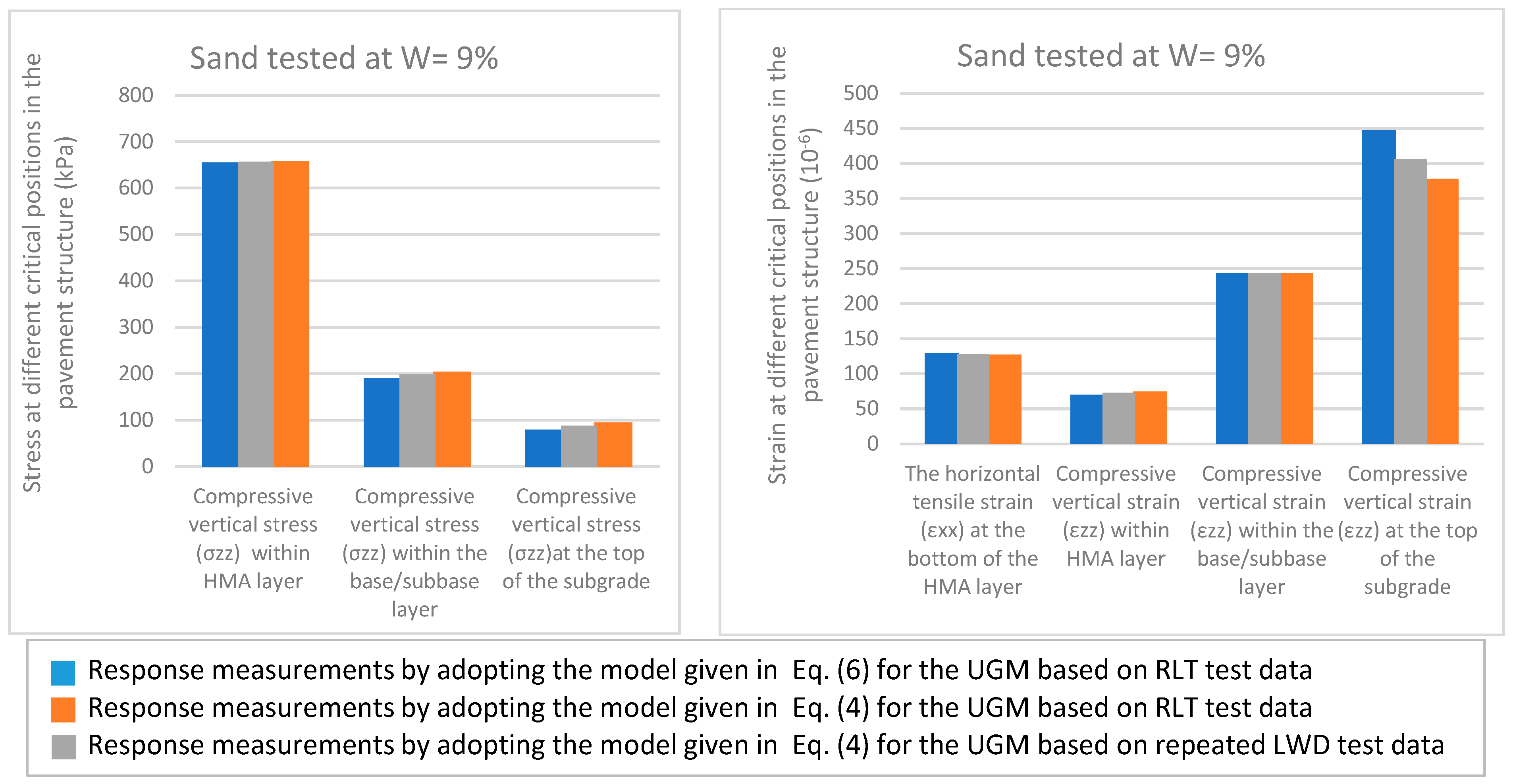
5.2. Observations in a Body of Sandy Subgrade Soil
Table 12 below shows the profile of the hypothetical pavement structure adopted to determine the response measurement when the sandy subgrade layer is considered as a stress-sensitive layer in ERAPAVE program.
5.2.1. For Sandy Subgrade Layer Compacted at 3% Water Content
Similar to the case of unbound base layers,
Table 13 shows k
1 and k
2 used in Equations (4) and (6) for the three chosen cases to be considered in this study together with the corresponding predicted layer moduli for the case of sandy subgrade soil compacted at 3% water content.
From
Table 13, it is evident that utilizing k
1 and k
2 from Equations (6) and Equation (4) for RLT testing resulted in resilient moduli of 192.9 kPa and 287.07 kPa, respectively. This represents a difference of about 39% between the moduli predicted by Equations (4) and (6) using the same RLT test data.
Moreover, when comparing the resilient modulus (Mr) calculated using Equation (4) based on RLT data (287.1 kPa) with the corresponding modulus calculated from Equation (4) based on LWD data (260.8 kPa), the percentage difference was approximately 9.5%. In other words, using LWD data led to a smaller percentage difference in Mr compared to the difference observed when employing two different models based on the same RLT test data.
Figure 7 shows the effect of calculated coefficients k
1 and k
2 from different tests and models on the response measurements at four critical positions within the pavement structure as defined in
Figure 1.
In
Figure 7, there is slight variation in stresses and strains at critical positions for various models (equations) except for the compressive vertical strain at the subgrade top. This strain was slightly higher with Equation (6) than Equation (4), using both RLT and LWD data.
This discrepancy in compressive vertical strain between Equation (4) and Equation (6) likely arises from the inherent differences in how these equations model the strains in the subgrade layer. Equation (6) may be more sensitive to specific factors, leading to higher predicted strain. Additionally, variations in material properties and assumptions embedded in the models can contribute to these differences.
5.2.2. For Sandy Subgrade Layer Compacted at 4% Water Content
Table 14 presents the values of k
1 and k
2 utilized in Equations (4) and (6) for the three selected cases under investigation in this study. Additionally, it displays the predicted layer moduli for the scenario involving sandy subgrade soil compacted at a 4% water content.
It can be seen from
Table 14 that the input data in terms of k
1 and k
2 from Equation (6) and Equation (4) for RLT testing have resulted in resilient modulus of 817.3 kPa and 1698.9 kPa, respectively (i.e., with about 70% present difference between the two adopted models given in Equations (4) and (6) based on the same RLT test data).
Comparing the modulus calculated from Equation (6) based on RLT data with the modulus calculated from the Equation (4) based on LWD data, the percentage difference will be about 21%.
Similarly, comparing the moduli calculated from Equation (4) based on RLT data with the corresponding moduli calculated from the same Equation (4) based on LWD data, the percentage difference was found to be about 50%. This also highlights that LWD data led to a smaller difference in resilient modulus compared to utilizing different models with the same RLT data.
Figure 8 shows the effect of calculated coefficients k
1 and k
2 from different tests and models on the response measurements at four critical positions within the pavement structure as defined in
Figure 1.
In
Figure 8, for sandy subgrade soil compacted at 4% water content, marginal variations in measured stresses and strains are observed at critical positions as illustrated in
Figure 1 for different adopted models (equations). However, a noticeable divergence is noticed in the case of compressive vertical strain at the top of the subgrade layer. This pattern aligns with the observations for sandy subgrade soil at 3% water content in
Figure 7. Specifically, the compressive vertical strain was slightly higher when using the model presented in Equation (6) compared to strains derived from adopting Equation (4) for both RLT and LWD data.
5.2.3. For Sandy Subgrade Layer Compacted at 9% Water Content
Table 15 displays the values of k
1 and k
2, which are utilized in Equations (4) and (6), respectively, for the three specific cases being examined in this study. It also includes the corresponding predicted layer moduli for the case involving compacted sandy subgrade soil with a 9% water content.
Table 15 illustrates that utilizing k
1 and k
2 from Equation (6) and Equation (4) for RLT testing yielded resilient moduli of 184.9 kPa and 261.95 kPa, respectively, showcasing a difference of approximately 34% between the moduli predicted by Equations (4) and (6) using the same RLT test data.
When comparing the modulus calculated from Equation (6) based on RLT data to that from Equation (4) based on LWD data, the percentage difference is approximately 20%. Likewise, comparing the moduli calculated from Equation (4) based on RLT data to the corresponding moduli calculated from the same Equation (4) based on LWD data shows a percent difference of about 14%. This implies that employing LWD resulted in a smaller percent difference in Mr compared to the difference observed when utilizing two different models based on the same RLT test data.
Figure 9 shows the effect of calculated coefficients k
1 and k
2 from different tests and models on the response measurements at four critical positions within the pavement structure as defined in
Figure 1.
In
Figure 9, observing sandy subgrade soil at 9% water content reveals slight variations in measured stresses and strains at critical positions shown in
Figure 1 for various adopted models (equations), except for compressive vertical strain at the subgrade layer’s top. This finding aligns with the cases of sandy subgrade soil compacted at 3% water content (
Figure 7) and 4% water content (
Figure 8). The strain was slightly higher for Equation (6) compared to strains derived using Equation (4) for both RLT and LWD data.
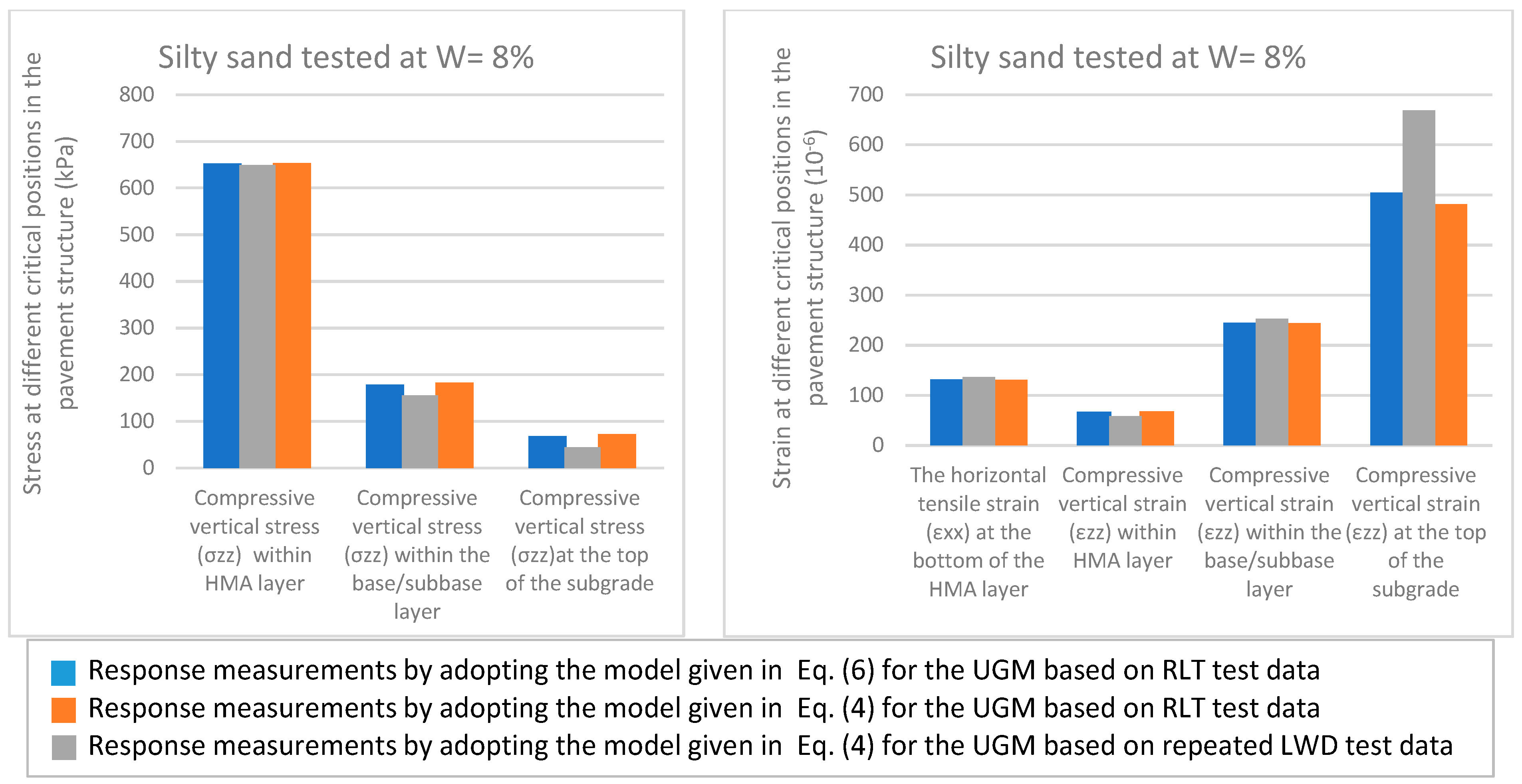
5.3. Observations in a Body of Silty Sandy Subgrade Soil
Table 16 below shows the profile of the hypothetical pavement structure adopted to determine the response measurement when the silty sand subgrade layer is considered as a stress-sensitive layer in ERAPAVE program.
5.3.1. For Silty Sandy Subgrade Layer Compacted at 8% Water Content
Table 17 exhibits the values of k
1 and k
2 applied in Equations (4) and (6) for the three selected cases under investigation in this study. It also presents the corresponding predicted layer moduli for the scenario where silty sand subgrade soil is compacted at 8% water content.
In
Table 17, the resilient moduli derived using k
1 and k
2 from Equation (6) and Equation (4) for RLT testing were 140.6 kPa and 157.06 kPa, respectively, indicating an 11% difference between these models based on the same RLT test data. When comparing moduli from Equation (6) with RLT data to those from Equation (4) with LWD data, there was a 70% difference. Similarly, comparing moduli from Equation (4) with RLT data to those from Equation (4) with LWD data showed an 80% difference. This emphasizes a significant divergence when calculating resilient moduli when utilizing LWD for silty sand compacted at 8% water content, compared to employing distinct models based on the same RLT data.
However, this large differences in calculated moduli by adopting LWD results lead to lower compressive vertical stress, and hence higher compressive vertical strain measurements at the top of the subgrade layer.
Figure 10 illustrates how the calculated coefficients k
1 and k
2 from various tests and models affect response measurements at four critical positions within the pavement structure as defined in
Figure 1.
In
Figure 10, specifically for the case of silty sand subgrade soil tested at 8% water content, utilizing LWD data in Equation (4) resulted in approximately 42% and 28% differences in compressive vertical stress and compressive vertical strain at the top of the subgrade layer, respectively, compared to the response measurements obtained by adopting Equation (6) with RLT test data.
5.3.2. For Silty Sandy Subgrade Layer Compacted at 10% Water Content
Table 18 illustrates the utilization of k
1 and k
2 in Equations (4) and (6) for the three designated cases in this study. Additionally, it showcases the predicted layer moduli corresponding to the scenario of compacted silty sand subgrade soil at 10% water content.
Table 18 reveals that using k
1 and k
2 from Equation (6) and Equation (4) for RLT testing yielded resilient moduli of 142.8 kPa and 160.69 kPa, respectively, presenting a 12% difference between the two models based on the same RLT test data.
Comparing the modulus calculated from Equation (6) based on RLT data with that from Equation (4) based on LWD data showed an 82% difference. Similarly, comparing moduli calculated from Equation (4) based on RLT data with those based on LWD data revealed a 92% difference. This highlights a substantial divergence when employing LWD for silty sand compacted at 10% water content, in contrast to using two distinct models based on RLT data. However, these significant differences in calculated moduli did not result in markedly noticeable differences in response measurements when utilizing the LWD model.
Figure 11 illustrates the impact of k
1 and k
2 coefficients from various tests and models on response measurements at four critical positions within the pavement structure as defined in
Figure 1.
In
Figure 11, examining silty sand subgrade soil tested at 10% water content, minor variations in measured stresses and strains at critical positions (
Figure 1) were observed for different models (equations), except for compressive vertical stress and strain at the top of the subgrade layer when using LWD data in Equation (4). The percentage differences were approximately 51% and 33% for compressive vertical stress and strain, respectively, compared to corresponding measurements using Equation (6) with RLT test data. Notably, the diversity in calculated response measurements for the silty subgrade soil increased with higher water content. This underlines the importance of adapting LWD in the Mechanistic–Empirical Pavement Design Guide, specifically for cohesive road materials, utilizing modified resilient modulus models that account for material properties such as water content.
6. Conclusions
The study focused on evaluating the effect of different factors on pavement response measurements using the ERAPAVE program. The key findings and observations for various scenarios were summarized:
The study employed an inclusive approach, utilizing an Excel problem solver to compute function constants (k1 and k2) for Equations (4) and (6). These constants, derived from resilient load triaxial (RLT) and lightweight deflectometer (LWD) tests, played a crucial role in accurately predicting response measurements within ERAPAVE.
At 3% water content, a 12% difference in stiffness moduli was observed between Equation (4) (RLT data) and Equation (6) (LWD data). This indicates that the use of LWD resulted in a smaller percentage difference in the stiffness moduli (Mr) calculated within ERAPAVE, in contrast to the larger difference observed when using two different models based on the same RLT test data. Minor discrepancies were noted in stresses and strains at critical positions for different models. However, using Equation (6) consistently predicted higher compressive vertical strain within the base/sub-base layer.
At 6% water content, the resilient moduli calculated using Equation (6) (RLT data) and Equation (4) (LWD data) showed similarity compared to the moduli calculated using Equation (4) with RLT data, influenced by water content as a critical factor. Water content was found to be a critical factor influencing the results. Doubling the water content of the base material from 3% to 6% halved the percentage difference in elastic moduli calculated using Equation (6) from RLT data and Equation (4) from LWD data (i.e., the percentage difference reduced from 12% to 5.6% with the doubling of water content).
LWD data resulted in a smaller percentage difference in resilient moduli (Mr) compared to different models based on RLT test data.
Slight variations in predicted stresses and strains were observed, except for the compressive vertical strain at the top of the subgrade, emphasizing the importance of model selection and consideration of specific conditions.
Resilient moduli calculated using LWD for silty sands at 8% and 10% water content differed significantly from other models based on RLT data. The presence of silt in the subgrade layer was identified as a significant factor affecting response measurements and resilient moduli, particularly with increasing water content. This highlights the importance of adapting the LWD in mechanistic–empirical pavement design, specifically for cohesive road materials, using modified resilient modulus models that take into account material properties such as water content.
7. Recommendations
Based on the findings in this study, several recommendations can be made to improve the integration of lightweight deflectometer (LWD) data into the Mechanistic–Empirical Pavement Design Guide:
Given the varying behavior of cohesive road materials with changing water content, it is imperative to develop modified resilient modulus models specifically designed for these materials. This adaptation should account for the influence of water content and material properties on response measurements.
Furthermore, calibration and validation of LWD data against traditional testing methods, such as repeated load triaxial (RLT) tests, should be conducted across a broad range of pavement materials and conditions. This will ensure that LWD can reliably predict layer moduli and response measurements. For cohesive materials, it is crucial to conduct LWD testing at different water content levels to understand their effect on response measurements. This will aid in refining the predictive models and improving the accuracy of the results.
By implementing these recommendations, the integration of LWD into the Mechanistic–Empirical Pavement Design Guide can be optimized, resulting in more accurate and efficient pavement designs.


