
A Review of Particle Packing Models and Their Applications to Characterize Properties of Sand-Silt Mixtures


Abstract
1. Introduction
2. Background
3. Review of Models
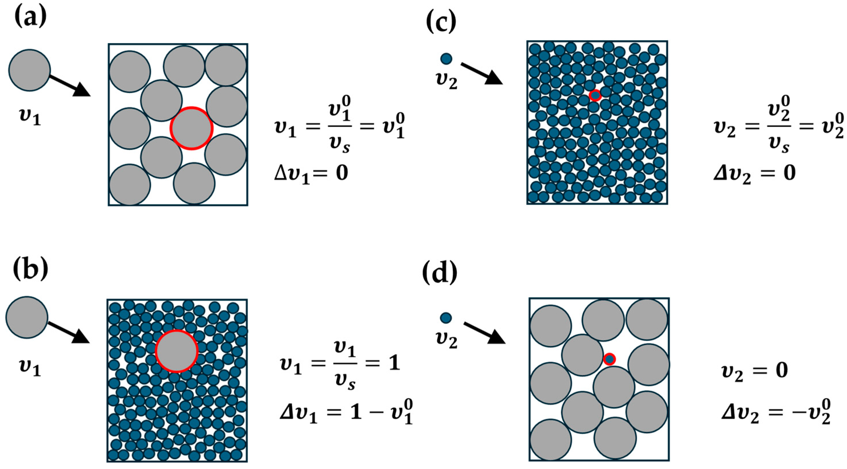
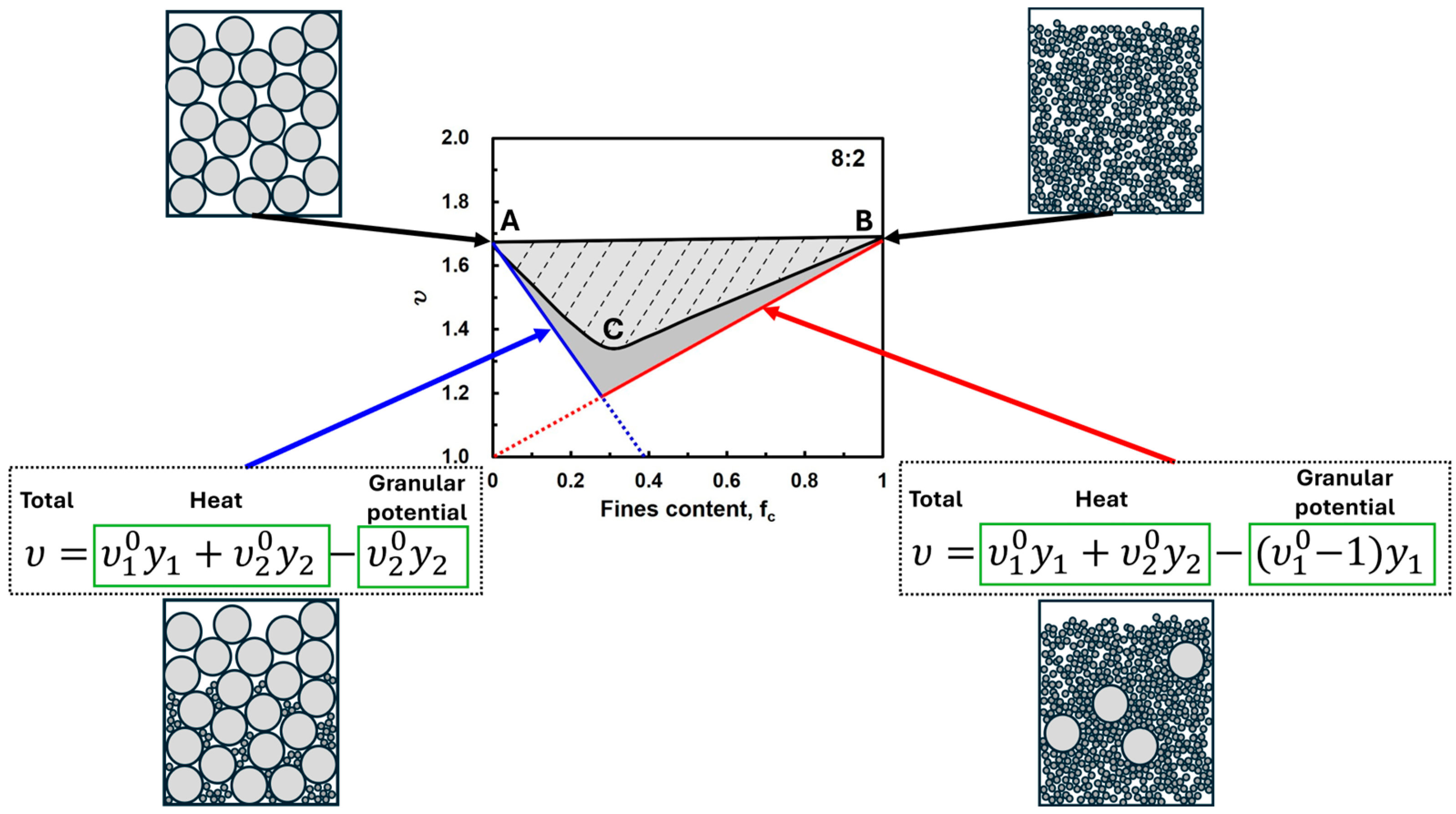
3.1. Limiting Cases
3.2. Linear Packing Models
3.3. Non-Linear Packing Models
3.3.1. Compressible Packing Models
3.3.2. Models with Non-Linear Functions
- Models with a single non-linear function
- 2.
- Models with two dominant packing structures
4. Geotechnical Application
4.1. Estimating Maximum, Minimum, and Critical State Void Ratios
4.2. Connection to Inter-Granular Void Ratio
4.3. Predicting Mechanical Properties and Relative Density
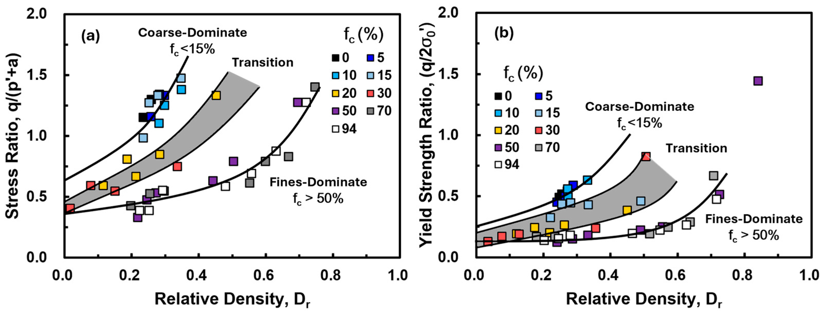
4.3.1. Stress Ratio and Yield Strength Ratio
- For < 15%, the behavior is coarse-grain dominant, similar to pure sand.
- For > 50%, the behavior is fine-grain dominant, similar to pure silt.
- For 15% << 50%, the behavior is a mix of the two, showing transitional characteristics.
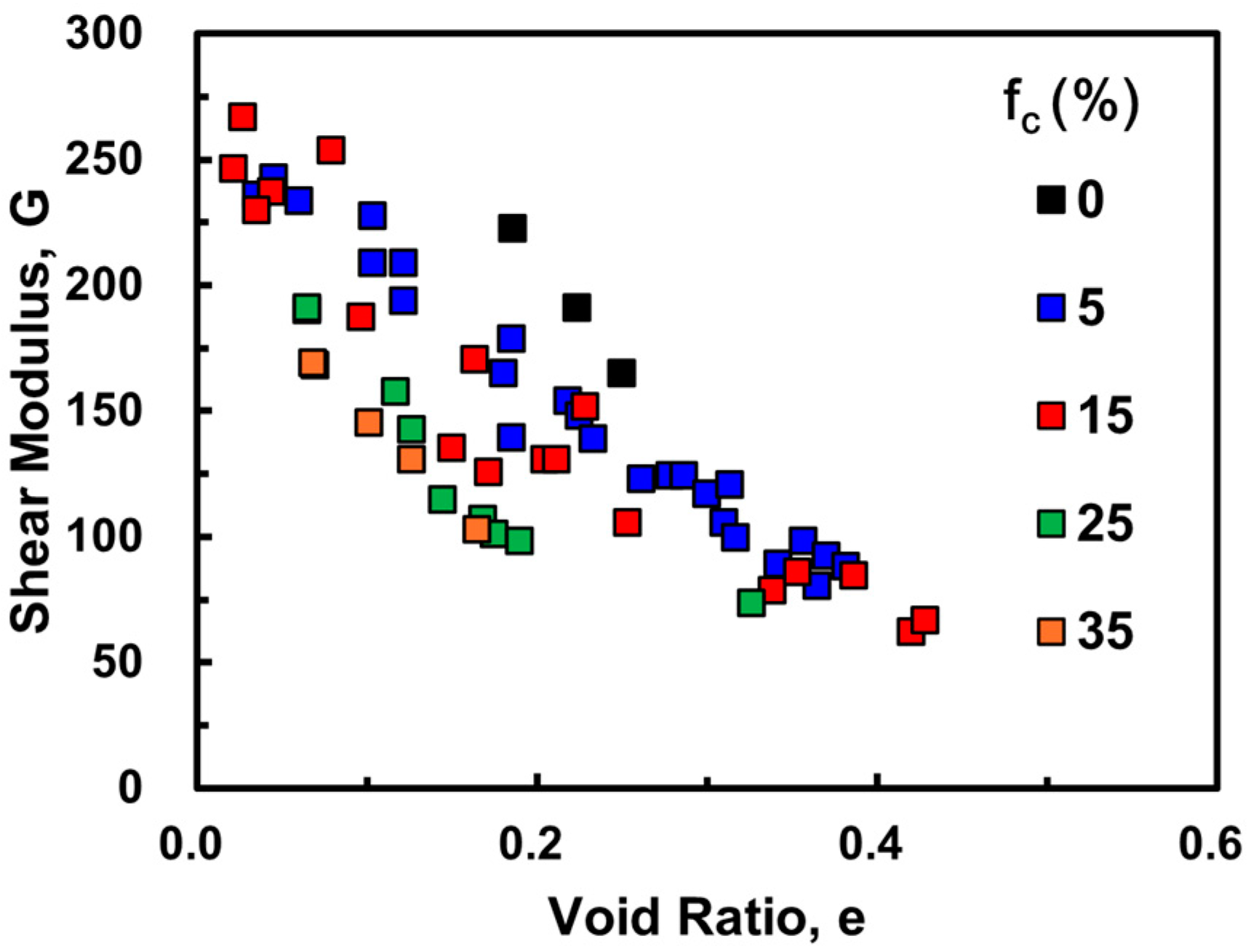
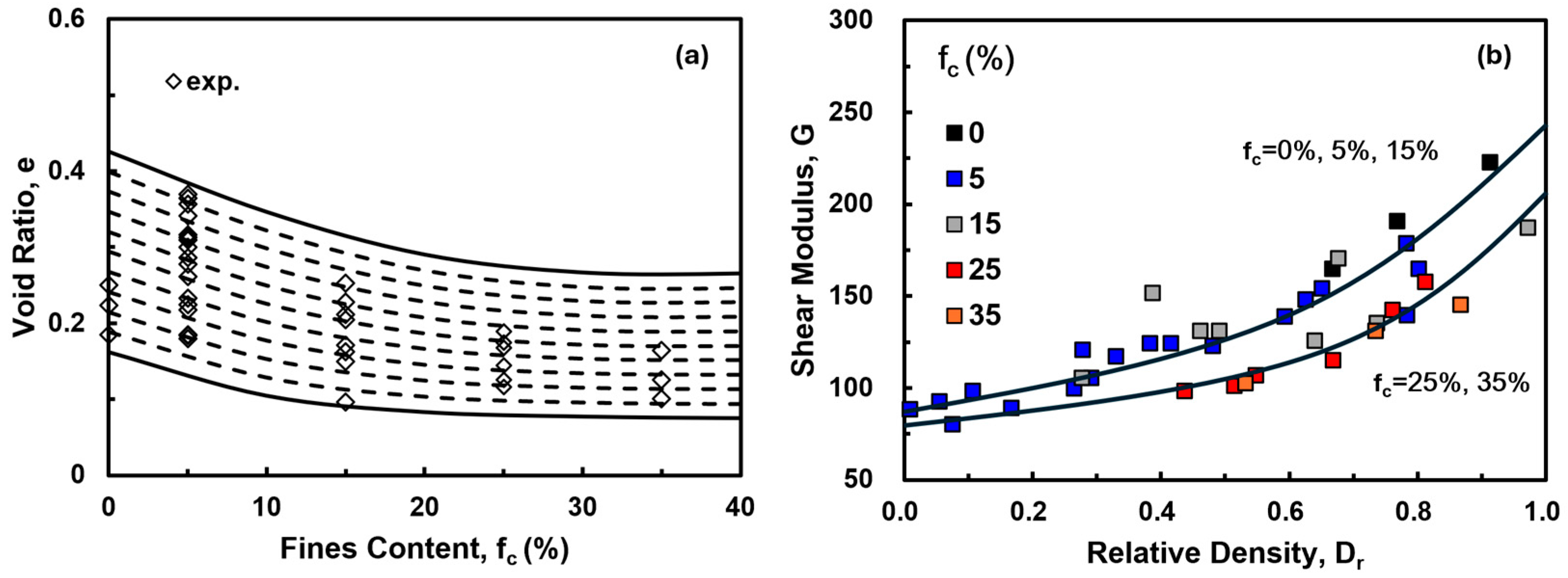
4.3.2. Shear Modulus
5. Conclusions
Author Contributions
Funding
Data Availability Statement
Acknowledgments
Conflicts of Interest
References
- de Larrard, F.; Sedran, T. Optimization of Ultra-High-Performance Concrete by the Use of a Packing Model. Cem. Concr. Res. 1994, 24, 997–1009. [Google Scholar] [CrossRef]
- Wang, Z.M.; Kwan, A.K.H.; Chan, H.C. Mesoscopic Study of Concrete I: Generation of Random Aggregate Structure and ®nite Element Mesh. Comput. Struct. 1999, 70, 533–544. [Google Scholar] [CrossRef]
- Du, W.; Singh, M.; Singh, D. Binder Jetting Additive Manufacturing of Silicon Carbide Ceramics: Development of Bimodal Powder Feedstocks by Modeling and Experimental Methods. Ceram. Int. 2020, 46, 19701–19707. [Google Scholar] [CrossRef]
- Liu, D.-M. Particle Packing and Rheological Property of Highly-Concentrated Ceramic Suspensions: Φm Determination and Viscosity Prediction. J. Mater. Sci. 2000, 35, 5503–5507. [Google Scholar] [CrossRef]
- Muzzio, F.J.; Shinbrot, T.; Glasser, B.J. Powder Technology in the Pharmaceutical Industry: The Need to Catch up Fast. Powder Technol. 2002, 124, 1–7. [Google Scholar] [CrossRef]
- Holtz, R.D.; Kovacs, W.D.; Sheahan, T.C. An Introduction to Geotechnical Engineering, 2nd ed.; Pearson: London, UK, 2011; ISBN 978-9332507617. [Google Scholar]
- Lade, P.; Liggio, C.; Yamamuro, J. Effects of Non-Plastic Fines on Minimum and Maximum Void Ratios of Sand. Geotech. Test. J. 1998, 21, 336–347. [Google Scholar] [CrossRef]
- Chang, C.S. Jamming Density and Volume-Potential of a Bi-Dispersed Granular System. Geophys. Res. Lett. 2022, 49, e2022GL098678. [Google Scholar] [CrossRef]
- Silbey, R.J.; Alberty, R.A.; Bawendi, M.G. Physical Chemistry, 4th ed.; Wiley: Hoboken, NJ, USA, 2004. [Google Scholar]
- Chang, C.S.; Deng, Y. Packing Potential Index for Binary Mixtures of Granular Soil. Powder Technol. 2020, 372, 148–160. [Google Scholar] [CrossRef]
- Chang, C.S.; Deng, Y. Compaction of Bi-Dispersed Granular Packing: Analogy with Chemical Thermodynamics. Granul. Matter 2022, 24, 58. [Google Scholar] [CrossRef]
- Westman, A.E.R.; Hugill, H.R. The Packing of Particles. J. Am. Ceram. Soc. 1930, 13, 767–779. [Google Scholar] [CrossRef]
- Furnas, C.C. Grading Aggregates—I.—Mathematical Relations for Beds of Broken Solids of Maximum Density. Ind. Eng. Chem. 1931, 23, 1052–1058. [Google Scholar] [CrossRef]
- Aïm, R.B.; Goff, P.L. Effet de Paroi Dans Les Empilements Désordonnés de Sphères et Application à La Porosité de Mélanges Binaires. Powder Technol. 1968, 1, 281–290. [Google Scholar] [CrossRef]
- Roquier, G. A Century of Granular Packing Models. Powder Technol. 2024, 441, 119761. [Google Scholar] [CrossRef]
- Stovall, T.; de Larrard, F.; Buil, M. Linear Packing Density Model of Grain Mixtures. Powder Technol. 1986, 48, 1–12. [Google Scholar] [CrossRef]
- Yu, A.B.; Zou, R.P.; Standish, N. Modifying the Linear Packing Model for Predicting the Porosity of Nonspherical Particle Mixtures. Ind. Eng. Chem. Res. 1996, 35, 3730–3741. [Google Scholar] [CrossRef]
- Larrard, F.D. Concrete Mixture Proportioning: A Scientific Approach; CRC Press: London, UK, 1999; ISBN 978-0-429-17909-9. [Google Scholar]
- Chang, C.S.; Wang, J.-Y.; Ge, L. Modeling of Minimum Void Ratio for Sand–Silt Mixtures. Eng. Geol. 2015, 196, 293–304. [Google Scholar] [CrossRef]
- Kim, M.; Seo, H. Evaluation of One- and Two-Parameter Models for Estimation of Void Ratio of Binary Sand Mixtures Deposited by Dry Pluviation. Granul. Matter 2019, 21, 71. [Google Scholar] [CrossRef]
- Roquier, G. The 4-Parameter Compressible Packing Model (CPM) Including a New Theory about Wall Effect and Loosening Effect for Spheres. Powder Technol. 2016, 302, 247–253. [Google Scholar] [CrossRef]
- Roquier, G. Evaluation of Three Packing Density Models on Reference Particle-Size Distributions. Granul. Matter 2024, 26, 7. [Google Scholar] [CrossRef]
- Toufar, W.; Born, M.; Klose, E. Contribution of Optimisation of Components of Different Density in Polydispersed Particles Systems; Freiberger: Saxony, Germany, 1976. [Google Scholar]
- Goltermann, P.; Johansen, V.; Palbøl, L. Packing of Aggregates: An Alternative Tool to Determine the Optimal Aggregate Mix. Mater. J. 1997, 94, 435–443. [Google Scholar] [CrossRef]
- Han, Q.W.; Wang, Y.C.; Xing, X.L. Initial Specific Weight of Deposits. J. Sediment. Res. 1981, 1, 1–13. [Google Scholar]
- Wu, W.; Li, W. Porosity of Bimodal Sediment Mixture with Particle Filling. Int. J. Sediment Res. 2017, 32, 253–259. [Google Scholar] [CrossRef]
- Kwan, A.K.H.; Chan, K.W.; Wong, V. A 3-Parameter Particle Packing Model Incorporating the Wedging Effect. Powder Technol. 2013, 237, 172–179. [Google Scholar] [CrossRef]
- Yu, A.B.; Standish, N. An Analytical—Parametric Theory of the Random Packing of Particles. Powder Technol. 1988, 55, 171–186. [Google Scholar] [CrossRef]
- Yu, A.B.; Standish, N. Estimation of the Porosity of Particle Mixtures by a Linear-Mixture Packing Model. Ind. Eng. Chem. Res. 1991, 30, 1372–1385. [Google Scholar] [CrossRef]
- Liu, Z.-R.; Ye, W.-M.; Zhang, Z.; Wang, Q.; Chen, Y.-G.; Cui, Y.-J. A Nonlinear Particle Packing Model for Multi-Sized Granular Soils. Constr. Build. Mater. 2019, 221, 274–282. [Google Scholar] [CrossRef]
- Chang, C.S.; Deng, Y. A Particle Packing Model for Sand–Silt Mixtures with the Effect of Dual-Skeleton. Granul. Matter 2017, 19, 80. [Google Scholar] [CrossRef]
- Chang, C.S.; Deng, Y. A Nonlinear Packing Model for Multi-Sized Particle Mixtures. Powder Technol. 2018, 336, 449–464. [Google Scholar] [CrossRef]
- Mooney, M. The Viscosity of a Concentrated Suspension of Spherical Particles. J. Colloid Sci. 1951, 6, 162–170. [Google Scholar] [CrossRef]
- Chang, C.S.; Wang, J.Y.; Ge, L. Maximum and Minimum Void Ratios for Sand-Silt Mixtures. Eng. Geol. 2016, 211, 7–18. [Google Scholar] [CrossRef]
- Thevanayagam, S.; Mohan, S. Intergranular State Variables and Stress–Strain Behaviour of Silty Sands. Géotechnique 2000, 50, 1–23. [Google Scholar] [CrossRef]
- Thevanayagam, S.; Martin, G.R. Liquefaction in Silty Soils—Screening and Remediation Issues. Soil Dyn. Earthq. Eng. 2002, 22, 1035–1042. [Google Scholar] [CrossRef]
- Yang, S.L.; Sandven, R.; Grande, L. Instability of Sand–Silt Mixtures. Soil Dyn. Earthq. Eng. 2006, 26, 183–190. [Google Scholar] [CrossRef]
- Yang, S.; Lacasse, S.; Forsberg, C.F. Application of Packing Models on Geophysical Property of Sediments. In Proceedings of the 16th International Conference on Soil Mechanics and Geotechnical Engineering, Osaka, Japan, 12–16 September 2005. [Google Scholar]
- Xenaki, V.C.; Athanasopoulos, G.A. Discussion of “Effects of Nonplastic Fines on the Liquefaction Resistance of Sands” by Carmine P. Polito and James R. Martin II. J. Geotech. Geoenviron. Eng. 2003, 129, 387–389. [Google Scholar] [CrossRef]
- Tao, M.; Fugueroa, J.L.; Saada, A.S. Influence of Nonplastic Fines Content on the Liquefaction Resistance of Soils in Terms of the Unit Energy. In Cyclic Behaviour of Soils and Liquefaction Phenomena; CRC Press: Boca Raton, FL, USA, 2004; pp. 223–231. [Google Scholar]
- Yang, S. Characterization of the Properties of Sand-Silt Mixtures. Ph.D. Thesis, Norwegian University of Science and Technology, Trondheim, Norway, 2004. [Google Scholar]
- Chang, C.S.; Deng, Y. Revisiting the Concept of Inter-Granular Void Ratio in View of Particle Packing Theory. Géotechnique Lett. 2019, 9, 121–129. [Google Scholar] [CrossRef]
- Han, D.; Nur, A.; Morgan, D. Effects of Porosity and Clay Content on Wave Velocities in Sandstones. Geophysics 1986, 51, 2093–2107. [Google Scholar] [CrossRef]


| Researcher(s) | Expression | Expression |
|---|---|---|
| Aim and Goff [14] | (Lower bound) | |
| Stovall et al. [16] | ||
| Yu et al. [17] | ||
| De Larrard [18] | ||
| Chang, Wang, and Ge [19] |
| Model Type | Strength/Limitation | Guideline on Size Ratio |
|---|---|---|
| Limiting Case Models | Simple and intuitive/Valid only for limiting case | Size ratio smaller than 0.1 or larger then 0.8 |
| Linear Packing Models | Accounts for interaction between particles/ In accurate in transition zone | Size ratio smaller than 0.2 |
| Non-Linear Packing Models | Captures more complex particle interactions/ Requires more parameters | Size ratio smaller than 0.8 or larger than 0.2 |
| Soil Type | Size (mm) | |||
|---|---|---|---|---|
| Sand | 0.44 | 0.949 | 0.572 | 4.0 |
| Silt | 0.032 | 1.480 | 0.770 | 4.0 |
| Soil Type | Size (mm) | |||
|---|---|---|---|---|
| Sandstone | 0.2 | 0.426 | 0.162 | 4.0 |
| Silty size clay | 0.015 | 0.480 | 0.100 | 4.0 |
Disclaimer/Publisher’s Note: The statements, opinions and data contained in all publications are solely those of the individual author(s) and contributor(s) and not of MDPI and/or the editor(s). MDPI and/or the editor(s) disclaim responsibility for any injury to people or property resulting from any ideas, methods, instructions or products referred to in the content. |
© 2024 by the authors. Licensee MDPI, Basel, Switzerland. This article is an open access article distributed under the terms and conditions of the Creative Commons Attribution (CC BY) license (https://creativecommons.org/licenses/by/4.0/).
Share and Cite
Chang, C.S.; Chao, J. A Review of Particle Packing Models and Their Applications to Characterize Properties of Sand-Silt Mixtures. Geotechnics 2024, 4, 1124-1139. https://doi.org/10.3390/geotechnics4040057
Chang CS, Chao J. A Review of Particle Packing Models and Their Applications to Characterize Properties of Sand-Silt Mixtures. Geotechnics. 2024; 4(4):1124-1139. https://doi.org/10.3390/geotechnics4040057
Chicago/Turabian StyleChang, Ching S., and Jason Chao. 2024. "A Review of Particle Packing Models and Their Applications to Characterize Properties of Sand-Silt Mixtures" Geotechnics 4, no. 4: 1124-1139. https://doi.org/10.3390/geotechnics4040057
APA StyleChang, C. S., & Chao, J. (2024). A Review of Particle Packing Models and Their Applications to Characterize Properties of Sand-Silt Mixtures. Geotechnics, 4(4), 1124-1139. https://doi.org/10.3390/geotechnics4040057