Uncertainty and Latin Hypercube Sampling in Geotechnical Earthquake Engineering

Abstract

A soil–foundation–structure system (SFSS) often exhibits different responses compared to a fixed-base structure when subjected to earthquake ground motion. Both kinematic and inertial soil–foundation–structure interactions can significantly influence the structural performance of buildings. Numerous parameters within an SFSS affect its overall response, introducing inherent uncertainty into the solution. Performing time history analyses, even for a linear elastic coupled SFSS, requires considerable computational effort. To reduce the computational cost without compromising accuracy, the use of the Latin Hypercube Sampling (LHS) technique is proposed herein. Sampling techniques are rarely employed in soil–foundation–structure interaction analyses, yet they are highly beneficial. These methodologies allow analyses determined by sampling to be conducted using commercial codes designed for deterministic analyses, without requiring any modifications. The advantage is that the number of analyses determined by the sampling size is significantly reduced as compared to considering all combinations of input parameters. After identifying the important samples, one can evaluate the seismic demand of selected soil–foundation–bridge pier systems using finite element numerical software. This paper indicates that LHS reduces computational effort by 60%, whereas structural response components (translation, rocking) show distinct trends for different systems.

1. Introduction

Rapid progress in earthquake engineering has significantly enhanced our ability to predict the performance of complex engineering structures under strong earthquake excitations. However, numerous uncertainties in the analysis of engineering systems can affect the results of a deterministic approach that relies on a single set of parameters. These uncertainties are even more pronounced in earthquake risk evaluations and include, among others, uncertainties in input motion [1,2,3,4] and soil properties [5,6,7,8,9].

The goal of the present study is not to address the general problem of uncertainties in earthquake engineering, nor to compare the various sampling methods available in the literature, but rather to evaluate Latin Hypercube Sampling (LHS) in contrast to the scenario where no sampling method is employed. Specifically, this paper compares LHS with an approach that considers all possible combinations of the input parameters. The aim is to highlight the advantages of using sampling techniques like LHS for parametric analyses.

In Monte Carlo analyses, a probabilistically based sampling procedure is typically used as a first step to develop a mapping from analysis inputs to analysis results [10,11,12,13]. In this study, Latin Hypercube Sampling, as proposed by Olsson and Sandberg [14], is employed to generate the sample size.

The results indicate that LHS can reduce computational effort by up to 60%, while differences in the output results between executing analyses for all possible combinations of input data and using the important samples are minimal (about 5%).

2. Uncertainty in Geotechnical Earthquake Engineering

The rapid progress in geotechnical and structural earthquake engineering has been instrumental in predicting the performance of complex structures under strong earthquake excitation. However, numerous uncertainties exist in the analysis of engineering systems which can affect the results of a deterministic approach that uses a single set of input parameters. For an earthquake risk assessment, these uncertainties are typically larger. In practice, scientists cannot predict the actual response of a structure but can only estimate a possible response under certain assumptions. The main sources of uncertainties relate to the lack of knowledge about how a real structure will behave under complex excitation. Uncertainties can be greater for existing structures than for modern structures since the building materials and techniques used are often poorly documented and potentially more variable than those in modern buildings.

Uncertainties are generally classified into two groups: aleatory (randomness) and epistemic (lack of knowledge) uncertainties [15]. Aleatory variability cannot be reduced, whereas epistemic uncertainty can be minimized through comprehensive data collection and proper modeling during the knowledge phase of the studied structure [16]. In general, in a stochastic model, uncertainty in the output vector arises from uncertainties in the input vector, model parameters, and model error. A comprehensive literature review on stochastic soil dynamics and its application in earthquake engineering can be found in [17].

For a soil–foundation–structure interaction (SFSI) system, the main uncertainties stem from real seismic loading and the random properties of the structure and soil materials. These two issues are discussed in the following paragraphs.

Uncertainties arising from structural and geotechnical properties, as well as ground motion characteristics, play an important role in predicting the overall performance of seismically excited structures [18,19]. The impact of different types of uncertainty on the seismic strength demand of an SFSI system, compared to a fixed-base system, is highlighted in [20]. It has been demonstrated that seismic demand depends on the earthquake input motion and whether soil–foundation–structure interaction effects are considered.

In the context of a stochastic soil–structure interaction analysis, kinematic interaction was investigated by Hoshiya and Ishii [21,22]. In their work, the system parameters were treated as random variables within Monte Carlo simulation methodologies. Harren and Fossun [23] used a probability integration technique, which requires less computational effort in an FEM than Monte Carlo simulation.

The goal of this paper is not to address the general problem of uncertainties in earthquake engineering, but rather to provide a brief review of issues related to the effect of uncertainties on a coupled soil–foundation–structure interaction system. Following the literature review, the use of the Latin Hypercube Sampling (LHS) methodology for soil–foundation–structure systems is proposed. Its efficiency in reducing the significant computational cost of finite element analyses is highlighted through specific examples.

2.1. Uncertainty in Input Motion

To account for the randomness of the input motion in the analysis, it is common to consider earthquakes as a random process defined by a corresponding power spectral density function or to use a significant number of earthquake records. Among the most significant pioneering contributions to the study of uncertainties is the work by Vanmarke [1] and the numerous publications that followed. The stochastic excitation described by the Kanai-Tajimi spectrum has often been used to define the input motion [2,3] studied in the stochastic response of embedded foundations using wave trains characterized by a spectral density function. Liang et al. [24] tested liquefaction under random loads, while Hao [25] studied the response of rigid plates to ground motions with specific variability described by the model of Harichandran and Vanmarke [26]. Ground motion prediction equations, represented by the standard deviation of the logarithmic residuals, exemplify the uncertainty (aleatory) in the input motion. One interesting tool to account for aleatory variability in ground motion is the vector approach to seismic hazard analyses proposed by Bazzurro and Cornell [4]. They proposed a methodology to evaluate the joint hazard of multiple ground motion parameters. Epistemic uncertainty in the estimation of ground motion for a single earthquake scenario is usually related, for practical engineering applications, to factors such as the choice of the ground motion prediction equation and the classification of surface geology within each geo-reference used to model the exposure. A logic tree approach is a common method used to address epistemic uncertainties. This method was used in the SHARE EU project [27]. The randomness in soil properties and the ground’s classification and stratification cannot be generalized and should be considered on a case-by-case basis.

2.2. Uncertainty in Soil Properties

Regarding geotechnical soil properties, aleatory uncertainty is influenced by the spatial variability of these properties, randomness in soil testing errors, and epistemic uncertainty related to several aspects such as a lack of information, the theoretical and practical shortcomings of the calculations, modeling errors, and the quality of available data. The literature offers numerous techniques for addressing these difficulties and uncertainties, usually tailored to different geotechnical problems. For example, Christian et al. [5] provide guidance for slope stability problems. The variability of each input parameter can be described by a statistical distribution with a mean and variance, which can be directly incorporated into the analysis. Vanmarcke [1] again provides methods for managing the consequences of spatial variability.

Wu et al. [28] presented an insightful example of evaluating alternative exploration programs to select the one that most effectively defines the site characteristics of a project. Statistical estimates of the variability in the designed soil properties have been proposed by Phoon and Kulhawy [6,7]. Based on extensive calibration studies, Phoon et al. [29] identified three ranges of soil property variability (low, medium, high) as sufficient to achieve reasonably uniform reliability levels for simplified checks. The extent to which a soil parameter value estimated from field tests or laboratory measurements varies is a crucial parameter. Several studies [30,31] provide tabulated coefficients of variation (COV) for soil parameters. Phoon and Kulhawy [6,7] categorized the uncertainty of soil properties to model soil variability effectively. The COV is the standard deviation divided by the mean, and its reported values range widely, only suggesting conditions at specific sites and not ones that are universally applicable.

In the study by Jones et al. [8], tabulated COV values of the inherent variability of several properties measured in the laboratory or through field tests can be found. Similar investigations have been conducted by other researchers, such as [1,9], and many others. Random fields are sometimes used to describe spatial variability. According to Baecher and Christian [9], applying random field theory to geotechnical issues assumes that the spatial variability of concern is the realization of a random field, defined as a joint probability distribution. The spatial dependency of a random field can be expressed via an autocorrelation function, which measures how a variable at one location correlates with itself at another location.

Another source of uncertainty arises from geotechnical calculation models. Although many geotechnical calculation models can reasonably predict complex soil–structure interaction behaviors through empirical calibrations, the correct choice of characteristic values significantly affects the overall safety of an engineering structure. Assimaki et al. [32] studied the effects of the spatial variability of soil properties on seismic wave propagation using a Monte Carlo simulation methodology and found that spatial variability highly influences the acceleration at the ground’s surface.

In summary, no simple method exists in engineering practice to account for soil’s randomness and uncertainty while ensuring that selected values achieve a predefined safety level. These values are provided from a design perspective as a first-order reliability analysis and are problem-dependent. If random variables can be included in the design process with minimal inconvenience, the definition of the characteristic value becomes a less critical issue. To evaluate the impact of earthquake variability on accuracy, a range of diverse ground motion records representing different magnitudes were incorporated into the model. This approach ensures that the analysis accounts for the broad spectrum of seismic activity. This approach is usually used in most parametric studies.

3. Methodologies

The most common methodologies used for estimating outputs while considering the uncertainties described in the previous paragraphs are Monte Carlo simulation methodologies. Monte Carlo simulations solve problems by generating a large number of random scenarios and observing the fraction of these scenarios that meet specified criteria. One of the most significant advantages of the Monte Carlo simulation method is its generality, despite it being time-consuming.

Implementing a Monte Carlo simulation methodology generally involves the selection of a model, the selection of the input parameters, the selection of probability distributions, repeated determinations, and the quantification of the model’s performance [8]. A large number of runs is necessary to cover the range of uncertainties and all possible combinations, ensuring that only realistic combinations of random parameters are considered. For risk evaluation, one can choose among various methods, including a reliability analysis or event tree analysis. The choice of method depends on the type of project and the available data. There are various probabilistic methods used in geotechnical engineering, each applicable to specific problems.

4. Sampling-Based Techniques

In a Monte Carlo analysis, a probabilistically based sampling procedure is employed to map analysis inputs to results [10,11,12,13]. Specifically, sampling-based techniques for uncertainty and sensitivity analyses involve five key steps, namely the definition of distributions, sample generation, the output’s evaluation, the display of uncertainty, and mapping exploration. In this study, Latin Hypercube Sampling (LHS) is utilized to generate the sample.

Once the sample is generated and the corresponding model evaluation using a finite element analysis is completed, the initial step of the uncertainty and sensitivity analyses is performed. The uncertainty analysis addresses the question of how the uncertainty in input parameters affects the uncertainty in output values. The sensitivity analysis, on the other hand, assesses the importance of individual input parameters relative to the uncertainty in the output parameters.

The mapping of input to output in an uncertainty analysis can be represented by single numbers or functions. For sensitivity analyses, the results can be represented using scatterplots, regression analyses, and statistical tests. In this study, scatterplots will represent the results. The analysis outcomes demonstrate the robustness of the uncertainty and sensitivity analysis results obtained using Latin Hypercube Sampling.

5. Latin Hypercube Sampling

Efficient sampling methods such as Latin Hypercube [33] and importance sampling are sometimes employed to reduce computational effort compared to traditional Monte Carlo sampling. However, the fundamental approach to estimating reliability remains consistent across these methods. Latin Hypercube Sampling was developed to address the need for uncertainty assessments in a specific class of problems. Consider variable Y, which might represent, for example, the acceleration demand considering SFSI effects, that is a function of the variables X₁, X₂, …, X_n (e.g., the structure’s height, mass, elastic modulus, shear wave velocity of soil, etc.). The main objective is to investigate how Y varies when Xn changes according an assumed joint probability distribution. A conventional method used to tackle this problem is Monte Carlo sampling. By repeatedly sampling from the assumed joint probability density function of the Xn and evaluating Y for each sample, one can estimate the distribution of Y, including its mean and other characteristics. While this approach provides reasonable estimates of Y’s distribution, it becomes computationally expensive when n is large because it requires a substantial number of evaluations.

To mitigate the computational cost, alternative methods like constrained Monte Carlo sampling have been developed. One such method is Latin Hypercube Sampling, introduced by [34]. LHS improves computational efficiency by systematically selecting sample points. In this approach, the range of each variable is divided into n non-overlapping intervals of equal probability. One value is randomly selected from each interval, ensuring that the full range of each variable is explored.

The n values obtained for each variable are then paired randomly. For example, if there are k variables X₁, X₂, …, X_k, the method generates n k-tuples, where each tuple represents a unique combination of values across all variables. These n k-tuples form an n×k matrix, where each row represents a specific set of values for the k input variables to be used in the computer model.

Figure 1 illustrates the generation of a sample size of 10 for a random vector k = [x, y, z]. The range of each variable is divided into 10 intervals with an equal probability content, as shown in Figure 1. One value is randomly sampled from each interval. The 10 values for x are paired randomly with the 10 values for y. These pairs are the combined randomly with the 10 values for z, resulting in 10 3-tuples. Figure 1a, Figure 1b, and Figure 1c depict the resulting xy, xz, and yz plans, respectively.

In the following paragraphs, the Latin Hypercube Sampling (LHS) methodology will be applied to an earthquake geotechnical engineering problem, specifically to a soil–foundation–structure (SFS) system similar to the one utilized in [35,36]. The primary objective of this application is to demonstrate the effectiveness of LHS in reducing the computational cost associated with the finite element analysis of coupled SFS systems while maintaining the accuracy of the results, such as periods, accelerations, and displacements.

5.1. Configuration of the Model

A single-degree-of-freedom (SDOF) structure is used, with the degree of freedom being the horizontal displacement of the structural mass ms. Of course, more complex systems, such as multi-degree-of-freedom structures or those exhibiting non-linear behavior, would offer additional insights [37]. However, the scope of this study is limited to provide a comparison between the Latin Hypercube Sampling (LHS) technique and the case where no sampling method is used in a simple, controlled scenario.

The SDOF structure is characterized by its stiffness ks, its dashpot coefficient cs, and its height h. The structure is founded on a rigid massless surface foundation of a width equal to 2B (Figure 2).

Two-dimensional plane strain analyses are performed in the time domain with Opensees software [38] to determine the elastic response of the structure. The elastic bedrock is modeled using Lysmer–Kuhlemeyer [1969] dashpots [39] at the base of the soil. The Lysmer–Kuhlemeyer dashpot is defined in Opensees based on the viscous uniaxial material model and the zero-length element formulation at the same node. Concerning vertical boundaries, I use the tied lateral boundary approach by declaring an equal degree of freedom for every pair of nodes which share the same y-coordinate, as described in Zienkiewicz et al., 1988 [40].

The size of the mesh was determined after a comprehensive sensitivity analysis. The geometry of the mesh is based on the concept of resolving the propagation of the shear waves at or below a pre-defined frequency, allowing an adequate number of elements to fit within the wavelength of the chosen shear wave. This ensures that the mesh is refined enough to capture propagating waves. For a maximum frequency of 10 Hz, I used quadratic elements of 1 m × 1 m, which suggest dense discretization. The soil mesh comprises 10,000 four-node quadrilateral elements. The width of the finite element soil mesh was large enough to avoid spurious reflections at the boundaries. The structure and the foundation are modeled by elastic beam elements of a 1 m length. Full connection is assumed between the foundation and the soil nodes.

The soil domain is homogeneous, with a thickness of H = 50 m. The bedrock has a shear wave velocity equal to Vs = 1500 m/s and a density equal to ρ = 2400 kg/m³. The foundation is a surface, rigid foundation and simulated by linear elastic beam elements and its width is equal to 6 m. The structure is simulated by linear elastic beam elements and its height in the current study is equal to 6 m. The structure’s mass is assumed to be lumped at the top of the pier. The damping for both the soil and structure is five per cent for the first mode of both the structure and soil profile (Rayleigh damping). The properties and the geometry of the studied models are depicted in Figure 2. The concrete elasticity modulus is equal to E = 32 GPa for all models. The soil’s density in all cases is equal to ρ = 2000 kg/m³ and its Poisson’s ratio equal to ν = 0.333. Three variables are considered as random and are modified: the mass at the top of the structure, m, in Mg; the shear wave velocity of the soil, vs., in m/s; and the diameter of the pier, d, in m. For this specific example, the following values are considered:

m = [100, 200, 400, 800, 1200] in Mg

(1)

Vs = [100, 200, 300, 400, 450] in m/s

(2)

d = [0.8, 1.2, 1.6, 2.0, 2.2] in m

(3)

All models are triggered at the level of the elastic half-space recorded by the Northridge 1994 earthquake record (NGA_1011), with fundamental period T_p = 0.16 s and a peak ground acceleration equal to amax = 0.95 m/s². The dynamic characteristics of the soil and structure change for each model, resulting at 125 different models to be studied. Each variable can have a different distribution. In this study, all three parameters are considered to have a uniform discrete distribution. In the following paragraphs, the efficiency of LHS is going to be evaluated.

5.2. Sample Generation

Considering all the combinations of the input parameters (mass m, diameter d, shear wave velocity Vs) results in 125 analyses. For these types of coupled systems, the computational effort is significant, as each analysis lasts for about 40 min on a standard computer. LHS is an efficient method that helps to reduce the computational effort required with minimal reduction in result accuracy. This method has rarely been used for coupled soil–foundation–structure interaction (SFSI) systems until now.

In the present study, analyses are run and results are compared in terms of the system’s periods, accelerations, and displacements, and for three cases:

(i)

All 125 combinations of the selected parameters.

(ii)

A total of 50 combinations resulting from the application of the LHS method 10 times, with 5 samples used each time (LHS1).

(iii)

A total of 50 samples resulting from a single application of the LHS method (LHS2).

For the aforementioned cases, elastic time history analyses were executed, and all necessary output parameters were calculated. The output parameters examined herein include the effective period for the flexible-base system, spectral acceleration, and spectral displacement for both the fixed-base and flexible-base systems.

5.3. Evaluation of LHS in Terms of Periods

The first examined output parameter is the effective period of the flexible-base system. Specifically, two approximations concerning the effective period of the system are evaluated: T_SFSI(FF) and T_SFSI(FND). T_SFSI(FF) is the effective period and T_SFSI(FND) is the pseudo-effective period.

The T_SFSI(FF) period for each analysis is obtained when dividing the Fourier spectrum at the top of the structure by the one at free-field conditions. This is the effective period as described by Veletsos et al. [41]. The numerical T_SFSI(FF) periods show excellent agreement with those derived from theoretical expressions [41], with differences of up to 6%. The T_SFSI(FND) period for each analysis is calculated by dividing the Fourier spectrum at the top of the structure by the one at the foundation level. The key difference between T_SFSI(FF) and T_SFSI(FND) is that T_SFSI(FND) includes only the displacement at the top of the structure relative to the foundation level, while T_SFSI(FF) also accounts for the horizontal displacement of the footing.

Figure 3a,b present the ratios of the effective and pseudo-effective to fixed-base periods in terms of the relative soil to structure stiffness ratio 1/σ = h/(T_FIXVs), where T_FIX is the fixed-base period of the structure, and in terms of the normalized structure mass, m_norm = m/(ρ h³), for all 125 combinations of the input parameters. It is worth noting that both the T_SFSI(FF)/T_FIX and T_SFSI(FND)/T_FIX ratios increase with either decreasing soil stiffness or increasing slenderness or mass of the structure. For actual soil profiles, the effective period of the system including an SFSI is up to eight times that of the fixed-base period, while the pseudo-effective period is up to six times that of the fixed-base period.

The LHS method provides very similar results for both the T_SFSI(FF)/T_FIX and T_SFSI(FND)/T_FIX ratios. For example, when the relative soil to structure stiffness ratio, 1/σ, is equal to 0.2, a common value for actual soil profiles, the resulting ratios for the effective and pseudo-effective to fixed-base period, for the five structure masses (m₁ to m₅), are as shown in

Table 1. Effective to fixed-base period ratios for the five mass (m₁ to m₅), assuming a 1/σ ratio equal to 0.2, when utilizing the three studied approaches: all combinations, LHS1, and LHS2.

	All	LHS1	LHS2
	TSFSI(FF)/TFIX	TSFSI(FF)/TFIX	TSFSI(FF)/TFIX
m1	2.5	2.5	2.4
m2	3.5	3.5	3.5
m3	4.2	4.5	5.0
m4	8.0	7.7	7.0
m5	10.0	10.8	10.0

and

Table 2. Pseudo-effective to fixed-base period ratios for the five mass (m₁ to m₅), assuming a 1/σ ratio equal to 0.2, when utilizing the three studied approaches: all combinations, LHS1, and LHS2.

	All	LHS1	LHS2
	TSFSI(FND)/TFIX	TSFSI(FND)/TFIX	TSFSI(FND)/TFIX
m1	2.1	2.0	2.0
m2	2.5	2.6	2.5
m3	3.5	3.5	3.7
m4	4.8	5.8	5.5
m5	6.3	6.7	6.2

, respectively. Assuming that the ‘correct’ value is the one derived from all combinations, it is evident from Table 1 and Table 2 that both LHS1 and LHS2 give a very good approximation of the period ratios, with differences ranging from 0 to 20%; in most cases, these differences are generally smaller than 5%.

5.4. Evaluation of LHS in Terms of Accelerations

The next output parameter examined for the assessment of the Latin Hypercube Sampling (LHS) methodology is the absolute acceleration at the top of the coupled soil–foundation–structure interaction (SFSI) system (üstr). This parameter is plotted on the same graph, with the absolute acceleration at the top of a fixed-base pier having a period equal to the pseudo-effective period T_SFSI(FND) subjected to free-field motion (üstr f). The ratio üstr/üstr f is an index of how the acceleration motion at the foundation level is affected by interaction effects [42]. The equations for all resulted radials are illustrated on the right side of the figure below. Figure 4b presents the same plots for the LHS1 case, and Figure 4c for the LHS2 case. Figure 4a shows the üstr/üstr f plot for all 125 combinations, with the results categorized according to the structure’s height to pier diameter (h/d) ratio. Each line represents the radial result after the linear regression of the scatterplots for each h/d ratio.

The results are expressed using the equation y = ax. The maximum percentage differences between the resulting ‘a’ factors from all the analyses compared to the ‘a’ factor from the LHS1 and LHS2 cases are 10% and 5.5%, respectively. Both LHS approaches are in a very good agreement with the exact solution (all combinations). However, the LHS2 case gives slightly better results for the same sample size. From Figure 4a it is evident that as the h/d ratio increases, the üstr/üstr f ratio also increases. This indicates that the more intense the interaction effects are, the more the acceleration time history at the foundation level is affected. Considering that, in the present study, the structure’s height is the same for all analyses, the h/d ratio is modified only through the modification of the pier diameter, d. Thus, as the h/d ratio increases the structure becomes more stiff.

When executing all 125 analyses, the time needed is approximately 5000 min. However, for the LHS1 and LHS2 cases, the time required is reduced by 60%, significantly lowering the computational effort needed while maintaining accuracy.

5.5. Evaluation of LHS in Terms of Displacements

The LHS methodology is also going to be evaluated in terms of the resulting displacements of the coupled SFSS. The examined ratios are the u_f/u_tot, the u_θ/u_tot, and u_sb/u_tot, where u_f, u_θ, and u_sb are the displacements at the top of the structure due to the horizontal movement of the foundation, due to the rocking of the foundation, and due to the structural bending, respectively, and the u_tot is the sum of the three above-mentioned displacements [36].

Figure 5a–c show the u_f/u_tot, u_θ/u_tot, and u_sb/u_tot ratios in terms of the relative soil to structure stiffness ratio for all examined normalized masses, considering all combinations. Figure 6a–c present the same results for the LHS1 case, while Figure 7a–c show the results for the LHS2 case.

The results from these figures are compelling and demonstrate the effective application of the LHS methodology, without significant differences in the final outcomes. Both the LHS1 and LHS2 cases give very good approximations of the displacement ratios, confirming the efficiency and reliability of the LHS methodology. Figure 8 and Figure 9 offer a detailed comparison between the results of LHS1, LHS2, and all 125 combinations for two specific normalized masses, m_norm = 1.85 and m_norm = 22.22. These comparisons are in terms of the effective period T_SFSI, u_f/u_tot, u_θ/u_tot, and u_sb/ u_tot, where u_f, u_θ, and u_sb are the displacement at the top of the structure due to the horizontal movement of the foundation, due to the rocking of the foundation, and due to structural bending, respectively, and the u_tot is the sum of the three above-mentioned displacements. The differences between these two masses are practically zero. This indicates that the LHS methodology provides an accurate and efficient means of estimating displacement ratios and other parameters in coupled soil–foundation–structure systems (SFSS).

6. Sample Size

In the existing literature, recommendations for sample sizes when using the Latin Hypercube Sampling (LHS) methodology are notably sparse. To ensure the accuracy of results when employing LHS, it is essential to determine an appropriate sample size, since the output is unknown until analyses with all combinations of the input parameters are executed.

For this evaluation, consider the soil–foundation–structure system depicted in Figure 2. The focus is on assessing how different sample sizes impact the acceleration results. The system features a mass of 400 Mg at the top of the structure, with the pier diameter and shear wave velocity of the soil profile defined by Equations (4) and (5). A total of 25 analyses were conducted on the coupled SFS system. The goal is to identify a sample size that provides a reliable approximation of the acceleration ratio.

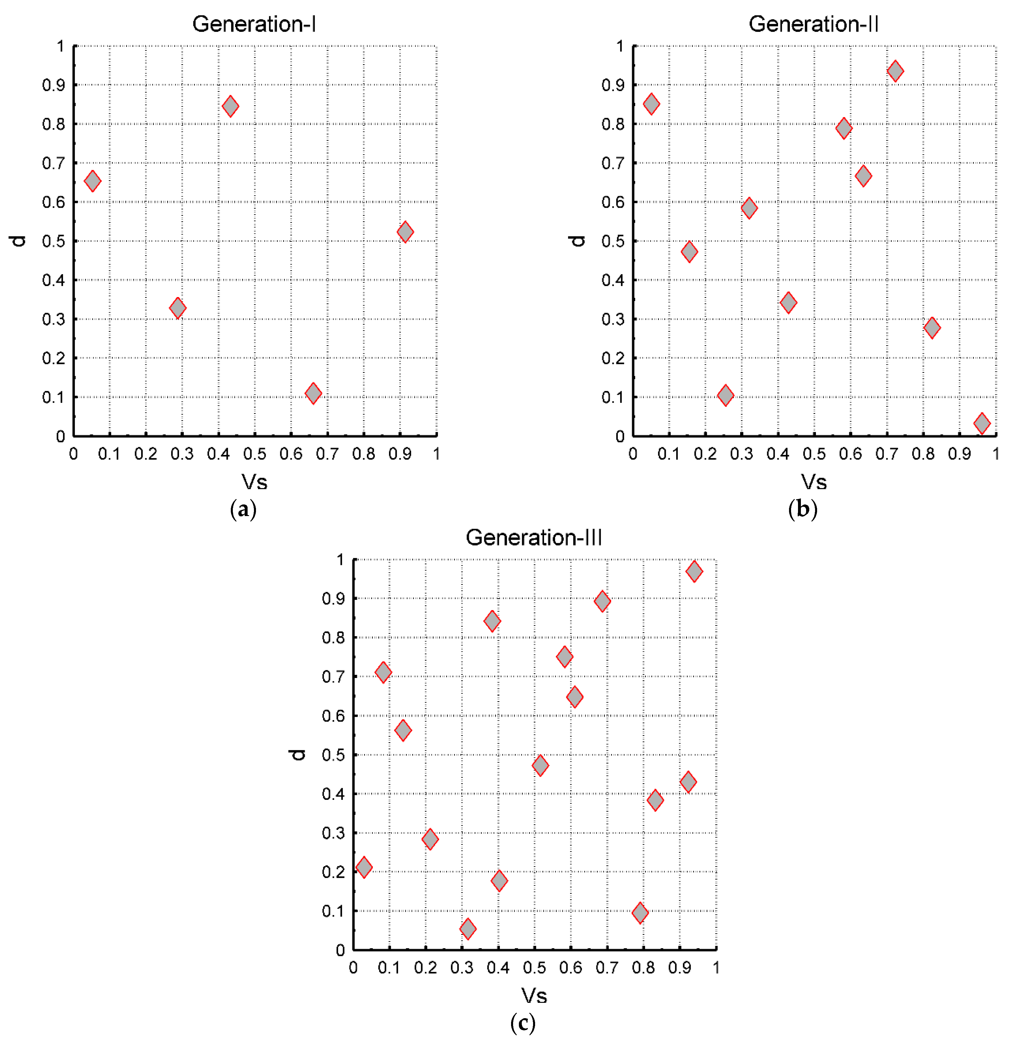
We then generated three sample sizes of 5, 10, and 15 samples using the LHS sample generation methodology. Figure 10 shows the generation of these three sample sizes. More specifically, Generation-I (Figure 10a) contains 5 samples, Generation-II (Figure 10b) contains 10 samples, and Generation-III (Figure 10c) contains 15 samples. Both the x-x and y-y axes of Figure 10 depict their probabilities. Following sample generation, time history analyses were performed for each sample size. In this paragraph, the üstr/üstr f ratio for the three samples and for all combinations is examined. Figure 11 presents the üstr/üstr f ratio, which is the result after the linear regression of the Ss, for all studied cases. It is evident that when the sample size is 15, the result is very close to the solution for all combinations, with its difference being equal to 2.5%. On the other hand, when we assume that the sample size is equal to 5, the difference from the exact solution is equal to 18%. The black continuous radial line is the 1:1 line. When the result is on this line, üstr = üstr f, which means that the response at the foundation level is actually the input to the superstructure, which is identical to both cases.

d = [0.8, 1.2, 1.6, 2.0, 2.2] in [m]

(4)

Vs = [100, 200, 300, 400, 450] in [m/s]

(5)

The results highlight the importance of choosing an appropriate sample size for the LHS methodology. A sample size of 15 offers a close approximation to the results obtained from all combinations, while a sample size of 5 results in a notable discrepancy. Therefore, selecting an adequate sample size is essential to ensure the accuracy and reliability of LHS in analyzing coupled soil–foundation–structure systems.

7. Discussion

The primary objective of this study was to evaluate the effectiveness of the Latin Hypercube Sampling (LHS) method in analyzing soil–foundation–structure interaction (SFSI) problems, and the results confirm its high efficacy. In its current application, the LHS methodology significantly reduced computational costs by 40% to 60%, with only a minor impact on accuracy—typically less than 5%—making it suitable for practical engineering applications. Of course, the computational cost mainly depends on the geometry of the studied systems, the meshing, the type of the analyses performed, and many other parameters. The study also revealed that for realistic soil profiles, the effective period of the system, including SFSI effects, can be up to eight times that of the fixed-base period, while the pseudo-effective period can be up to six times that.

In this paper, it is highlighted that sampling techniques, such as Latin Hypercube Sampling (LHS), offer significant advantages in soil–foundation calculations by improving the computational efficiency and coverage of the variable space and systematically selecting sample points across the full range of each variable, ensuring that the variability of inputs (e.g., soil properties, structure mass, and foundation characteristics) is better represented with fewer simulations. This reduces the variance of the results and allows engineers to obtain reliable estimates of important parameters such as periods, accelerations, and displacements in soil–foundation–structure interaction (SFSI) systems with a lower number of model evaluations. However, there are significant challenges in applying sampling techniques to soil–foundation–structure calculations. Soil behavior is inherently complex and highly variable, exhibiting non-linearity, heterogeneity, and uncertainty in key parameters such as its shear wave velocity. Assigning accurate probability distributions to these variables is critical but difficult, and errors in these assumptions can impact the reliability of the results. In addition, the effectiveness of sampling techniques relies heavily on the calibration of the computational model to real-world data, and this requires thorough testing and validation. In summary, while LHS offers clear benefits in reducing computational effort and providing accurate estimates, the complexity of soil properties and the need for precise calibration present significant challenges.

In using the Latin Hypercube Sampling (LHS) technique, several key parameters impact its effectiveness and accuracy. The number of samples chosen affects the precision and reliability of the results. More samples generally lead to a better coverage of the input space and more accurate estimates but require more computational resources. The range of each input variable is divided into equal probability intervals. The quality of the sampling depends on how well these intervals represent the variability of the input variables. Proper division ensures that the entire range is explored uniformly. LHS involves randomly pairing values from different intervals. The effectiveness of this random pairing influences how well the sampling represents the joint distribution of the input variables. Consistent and random pairing helps avoid biases and ensures comprehensive coverage. Assumptions about the probability distributions of input variables (e.g., uniform, normal) also affect the accuracy of the LHS technique. Accurate distribution modeling is crucial for obtaining reliable results. The number of input variables affects the complexity of the sampling. Higher-dimensional problems may require more careful sampling to ensure that interactions between variables are adequately represented. Overall, these parameters influence the balance between computational efficiency and the accuracy of the results obtained using LHS. The proper tuning of these factors is essential for optimizing the performance of the LHS technique.